Application of the Tomtit Flock Metaheuristic Optimization Algorithm to the Optimal Discrete Time Deterministic Dynamical Control Problem

Abstract

A new bio-inspired method for optimizing the objective function on a parallelepiped set of admissible solutions is proposed. It uses a model of the behavior of tomtits during the search for food. This algorithm combines some techniques for finding the extremum of the objective function, such as the memory matrix and the Levy flight from the cuckoo algorithm. The trajectories of tomtits are described by the jump-diffusion processes. The algorithm is applied to the classic and nonseparable optimal control problems for deterministic discrete dynamical systems. This type of control problem can often be solved using the discrete maximum principle or more general necessary optimality conditions, and the Bellman’s equation, but sometimes it is extremely difficult or even impossible. For this reason, there is a need to create new methods to solve these problems. The new metaheuristic algorithm makes it possible to obtain solutions of acceptable quality in an acceptable time. The efficiency and analysis of this method are demonstrated by solving a number of optimal deterministic discrete open-loop control problems: nonlinear nonseparable problems (Luus–Tassone and Li–Haimes) and separable problems for linear control dynamical systems.

1. Introduction

Global optimization algorithms are widely used to solve engineering, financial, optimal control problems, as well as problems of clustering, classification, deep machine learning and many others [1,2,3,4,5,6,7,8,9,10]. To solve complex applied problems, both deterministic methods of mathematical programming [11,12,13] and stochastic metaheuristic optimization algorithms can be used [14,15,16,17,18,19,20,21,22,23,24,25,26]. The advantage of the methods of the first group is their guaranteed convergence to the global extremum, and the advantage of the second group is the possibility of obtaining a good-quality solution at acceptable computational costs, even in the absence of convergence guarantees. Among metaheuristic optimization algorithms, various groups are conventionally distinguished: evolutionary methods, swarm intelligence methods, algorithms generated by the laws of biology and physics, multi-start, multi-agent, memetic, and human-based methods. The classification is conditional, since the same algorithm can belong to several groups at once. Four characteristic groups of metaheuristic algorithms can be distinguished, in which heuristics that have proven themselves in solving various optimization problems are coordinated by a higher-level algorithm.

Evolutionary methods, in which the search process is associated with the evolution of a solutions set, named a population, include Genetic Algorithms (GA), Self-Organizing Migrating Algorithm (SOMA), Memetic Algorithms (MA), Differential Evolution (DE), Covariance Matrix Adaptation Evolution Strategy (CMAES), Scatter Search (SS), Artificial Immune Systems (AIS), Variable Mesh Optimization (VMO), Invasive Weed Optimization (IWO), and Cuckoo Search (SC) [3,4,14,15,16,17,18,20].

The group of Swarm Intelligence algorithms includes Particle Swarm Optimization (PSO), Ant Colony Optimization (ACO), Artificial Bee Colony (ABC), Bacterial Foraging Optimization (BFO), Bat-Inspired Algorithm (BA), Fish School Search (FSS), Cat Swarm Optimization (CSO), Firefly Algorithm (FA), Gray Wolf Optimizer (GWO), Whale Optimization Algorithm (WOA), Glowworm Swarm Optimization (GSO), Shuffled Frog-Leaping Algorithm (SFLA), Krill Herd (KH), Elephant Herding Optimization (EHO), Lion Pride Optimization Algorithm (LPOA), Spotted Hyena Optimizer (SHO), Spider Monkey Optimization (SMO), Imperialist Competitive Algorithm (ICA), Stochastic Diffusion Search (SDS), Human Group Optimization Algorithm (HGOA), and Perch School Search Algorithm (PSS). In the methods of this group, swarm members (solutions) exchange information during the search process, using information about the absolute leaders and local leaders among neighbors of each solution and their own best positions [2,15,16,17,20,22,23,24,25,26,27,28].

The group of physics-based algorithms includes Simulated Annealing (SA), Adaptive Simulated Annealing (ASA), Central Force Optimization (CFO), Big Bang-Big Crunch (BB-BC), Harmony Search (HS), Fireworks Algorithm (FA), Grenade Explosion Method (GEM), Spiral Dynamics Algorithm (SDA), Intelligent Water Drops Algorithm (IWD), Electromagnetism-like Mechanism (EM), and the Gravitational Search Algorithm (GSA) [15,16,17,19,23,24,25,26,27,28].

The group of multi-start-based algorithms includes Greedy Randomized Adaptive Search (GRAS) and Tabu Search (TS) [15,16,17].

Among these four groups, bio-inspired optimization algorithms can be distinguished as a part of nature-inspired algorithms [2,7,15,22,23,24,25,26,27,28]. In turn, among bio-inspired methods, bird-inspired algorithms that imitate the characteristic features of the behavior of flocks of various birds during foraging, migration, and hunting are widely used: Bird Mating Optimizer (BMO), Chicken Swarm Optimization (CSO), Crow Search Algorithm (CSA), Cuckoo Search (CS), Cuckoo Optimization Algorithm (COA), Emperor Penguin Optimizer (EPO), Emperor Penguins Colony (EPC), Harris Hawks Optimization (HHO), Migrating Bird Optimization (MBO), Owl Search Algorithm (OSA), Pigeon Inspired Optimization (PIO), Raven Roosting Optimization (RRO), Satin Bowerbird Optimizer (SBO), Seagull Optimization Algorithm (SOA), and the Sooty Tern Optimization Algorithm (STOA) [15,24,25,26].

One of the applications of bio-inspired optimization algorithms is the problem of finding control laws for discrete dynamical systems [1,10]. As a rule, to solve this class of optimal control problems, the necessary optimality conditions are applied, which are reduced to solve a boundary value problem for a system of difference equations. For systems with convex varying, the discrete maximum principle is applied. An alternative way is to apply sufficient optimality conditions in the form of the Bellman’s equation. In this case, the optimal control found in the form of feedback depends on the state vector of the system, which is more preferable. However, it is well known that with an increase in the state vector dimension, the computational costs of using the dynamic programming procedure increase significantly. Special problems are caused by the solution of nonseparable problems, as well as problems in which the vector variation is not convex and, therefore, the discrete maximum principle is not valid. Since the problem of optimal control of discrete systems is finite dimensional, the use of efficient bio-inspired optimization methods for its resolution is natural.

The article is devoted to the development of the swarm intelligence and bird-inspired groups of methods based on observing the process of searching for food by a flock of tomtits, organizing their sequential movement under the influence of the leader of the flock. To simulate the trajectories of movement of each tomtit, the solution of a stochastic differential equation with jumps is used. The parameters of the random process—the drift vector and the diffusion matrix—depend on the position of all members of the flock and their individual achievements. The method is hybrid because it also uses the ideas of particle swarm optimization methods [15,16,17], methods that imitate the behavior of cuckoos with Levy flights [29], and the Luus–Jaakola method with successive reduction and further incomplete restoration of the search area [1]. Based on the assertion of the Free Lunch Theorem [30], it can be argued that the problem of developing new efficient global optimization algorithms used to solve complex optimal control problems remains relevant. In particular, the method should allow us to solve both separable and non-classical nonseparable optimization problems for discrete deterministic dynamical control systems [1,10]. As a benchmark of problems for assessing the accuracy of the method and computational costs, a set of nonlinear nonseparable and classical linear separable problems with known best or exact solutions was used.

The paper is organized as follows. Section 2.1 contains the statement of the discrete deterministic open-loop control problem. Section 2.2 provides a description of the solution search strategy and a step-by-step novel bio-inspired metaheuristic optimization method. In Section 3, the application of the new optimization method described in Section 2.2 for the representative set of optimal control problems described in Section 2.1 is given. Recommendations on the choice of method hyperparameters are given, time costs are estimated to obtain numerical results of acceptable quality, and comparison with the results obtained by other known metaheuristic algorithms is presented.

2. Materials and Methods

2.1. Open-Loop Control Problem

Let us consider a nonlinear discrete deterministic dynamical control system described by a state equation of the form

$$x(t+1)=f(t,\hspace{0.17em}\hspace{0.17em}x(t),\hspace{0.17em}\hspace{0.17em}u(t)), t=0,1,\dots ,N-1,$$

(1)

where $t$ is a discrete time with number of stages $N$; $x$ is the $(n\times 1)$ state vector; $u$ is the $(q\times 1)$ control vector, $u\in U(t)=[a_1(t),\hspace{0.17em}\hspace{0.17em}{b}_1(t)]\times \dots \times [a_q(t),\hspace{0.17em}\hspace{0.17em}{b}_q(t)];$ $f_i(t,\hspace{0.17em}\hspace{0.17em}x,\hspace{0.17em}\hspace{0.17em}u),i=1,\dots ,n$ are a known continuous functions.

Initial condition:

$$x(0)=x_0.$$

(2)

Let us define a set $D(0,\hspace{0.17em}\hspace{0.17em}{x}_0)$ of pairs $d=(x(\cdot ),\hspace{0.17em}\hspace{0.17em}u(\cdot )),$ where $x(\cdot )=\{x_0,\hspace{0.17em}\hspace{0.17em}x(1),\dots ,x(N)\}\hspace{0.17em}$ is a trajectory, $u(\cdot )=\{u(0),\hspace{0.17em}\hspace{0.17em}u(1),\hspace{0.17em}\hspace{0.17em}\dots ,\hspace{0.17em}\hspace{0.17em}u(N-1)\}$ is an open-loop control, satisfying the state equation (1) and initial condition (2).

The performance index to be minimized is defined on the set $D(0,x_0)$ as

$$I(d)={\displaystyle \sum _{t=0}^{N-1}{f}^0(t,\hspace{0.17em}\hspace{0.17em}x(t),\hspace{0.17em}\hspace{0.17em}u(t))+F(x(N))},$$

(3)

or

$$I(d)=F(x(0),\dots ,x(N);\hspace{0.17em}\hspace{0.17em}u(0),\dots ,u(N-1)),$$

(4)

where $f^0(t,\hspace{0.17em}\hspace{0.17em}x,\hspace{0.17em}\hspace{0.17em}u),\hspace{0.17em}\hspace{0.17em}F(x),\hspace{0.17em}\hspace{0.17em}F(x(\cdot ),\hspace{0.17em}\hspace{0.17em}u(\cdot ))$ are known continuous functions. The notation form (3) is typical for separable optimal control problems, and the form (4) is typical for nonseparable ones.

It is required to find an optimal pair $d^{*}=(x^{*}(\cdot ),\hspace{0.17em}\hspace{0.17em}{u}^{*}(\cdot ))\in D(0,\hspace{0.17em}\hspace{0.17em}{x}_0)$ that minimizes the performance index, i.e.,

$$I(d^{*})=\underset{d\in D(0,x_0)}{\min }I(d).$$

(5)

To solve the problem (5), an algorithm that imitates the behavior of a tomtits flock is proposed. This algorithm belongs to the nature-inspired (more precisely, bird-inspired) and swarm intelligence metaheuristic optimization algorithms [2,15,16,17]. This problem was solved using iterative dynamic programming and the Luus–Jaakola algorithm [1] and by the Perch School Search optimization algorithm [10]. The results of a comparative analysis of the obtained results are presented below in the solved examples.

2.2. Bio-Inspired Metaheuristic Optimization Method

The problem of finding the global minimum of the objective function $f(x)=f(x_1,\dots ,x_n)$ on the set of feasible solutions of the form $D=[a_1,b_1]\times \cdots \times [a_n,b_n]$ is considered.

The Tomtit Flock Optimization (TFO) method of simulating the behavior of a flock of tomtits is a hybrid algorithm for finding the global conditional extremum of functions of many variables, related to both swarm intelligence methods and bio-inspired methods.

A tomtit unites in flocks. They obey the commands of the flock leader and have some freedom in choosing the way to search for food. Tomtits are distinguished from other birds and animals by their special cohesion, coordination of collective actions, intensity of use of the food source found until it disappears, and clear and friendly execution of commands common to members of the flock.

Finite sets $I=\{x^j={(x_1^j,x_2^j,\dots ,x_n^j)}^T,j=1,2,\dots ,NP\}\subset D$ of possible solutions, named populations, are used to solve the problem of finding a global constrained minimum of objective function, where $x^j$ is a tomtit-individual (potential feasible solution) with number $j$, and $NP$ is a population size.

In the beginning, when number of iterations $k=0$, the method creates initial population of tomtits via the uniform distribution law on a feasible solutions set $D$. The value of objective function $f(x)$ is calculated for each tomtit, which is a possible solution. The solution with the best value of objective function is the position of flock leader. The leader does not search for food in the current iteration. It waits for results of finding food for processing results and further storage in the memory matrix:

$$\left(\begin{array}{cccc}{x}_1^1& \cdots & x_n^1& f(x^1)\\ ⋮& \ddots & ⋮& ⋮\\ x_1^K& \cdots & x_n^K& f(x^K)\end{array}\right).$$

The memory matrix size is $K\times (n+1)$, where $K$ is a given maximum number of records. The best achieved result on each $k$-th iteration is added in the matrix until the matrix is fulfilled. The number $K$ defines the iterations counted in one pass. Results in the matrix are ordered by the following rule. The first record in the matrix is the best solution $(x^1,f(x^1))$; other records are ordered by increasing (nondecreasing) value of the objective function. When the memory matrix is fulfilled, the best result is placed in a special set Pool (set of the best results of passes), after which the matrix is cleared.

New position of the leader is randomly generated by Levy distribution [29]:

$$x_i^{1,k+1}=x_i^{1,k}+\frac{\mathsf{\alpha }}{k+1}\cdot Lev{y}_i(\mathsf{\lambda }),\hspace{1em}i=1,\dots ,n,$$

where $x_i^{1,k}$ is a coordinate of the leader’s position on the $k$-th iteration, and $\mathsf{\alpha }$ is a movement step, $\mathsf{\lambda }\in \left(1,3\right]$. Studies of animal behavior have shown that the Levy distribution most accurately describes the trajectory of birds and insects. Due to the “heavy tails” of the Levy distribution, the probability of significant deviations of the random variable from the mean is high. Therefore, according to the above expression, sufficiently large increments are possible for each coordinate of the vector $x^{j,k}.$ If the new value of the certain coordinate does not belong to the set of feasible solutions; that is $x_i\notin \left[a_i,b_i\right],$ then one should repeat the generation process.

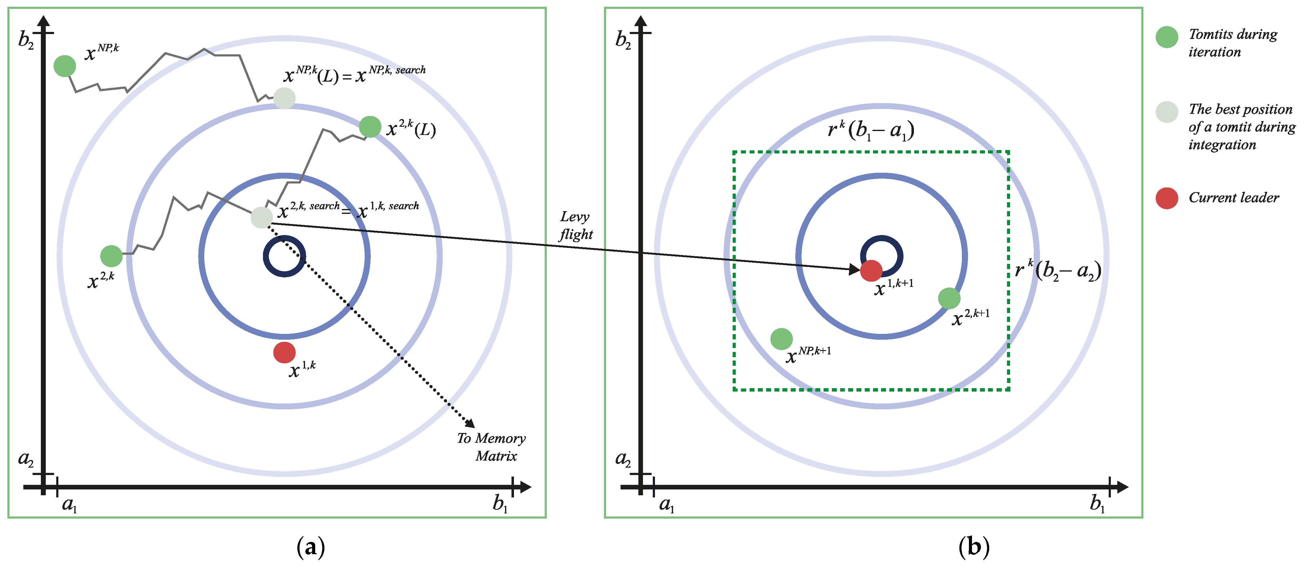
This process describes the flight of the flock leader from one place to another. Other tomtits fly after it at the command of the leader. Positions of these tomtits are modeled using a uniform distribution on the parallelepiped set. The center of the parallelepiped set is determined by the position of the leader of the flock; the lengths of the sides are equal $r^k(b_i-a_i)$, $i=1,\dots ,n$, where $r^{k+1}=\mathsf{\gamma }\hspace{0.17em}{r}^k$, $\hspace{0.17em}{r}^0=1$, $\mathsf{\gamma }$—reduction parameter of search set; if $r^k<\mathsf{\epsilon }$, then the current pass is stopped and a new one starts. Upon reaching $K$ iterations or when the condition $r^k<\mathsf{\epsilon }$ is fulfilled, the pass is considered complete, the counter of passes is increased: $p=p+1$, and the parameter that describes the size of the next search space is set equal to $r^0={\mathsf{\eta }}^p$, where $\mathsf{\eta }$—reconstruction parameter of search set. The found coordinate values determine the initial conditions for the search at the current iteration (the initial position of each tomtit).

It is assumed that each $j$-th individual has a memory that stores:

• Current iteration count $k$;
• Current position $x^{j,k}$ and the corresponding value of objective function $f(x^{j,k})$;
• The best position $x^{best}$ and the corresponding value of objective function in population $f(x^{best})$;
• The best position of a tomtit $x^{j,best}$ during all iterations and the corresponding value of objective function $f(x^{j,best})$;
• The best position $x^{j,local}$ among all tomtits located in the vicinity of the $j$-th individual of radius $\mathsf{\rho }$ and the corresponding value of objective function $f(x^{j,local})$.

The trajectory of movement of each individual (for all tomtits $j=1,\dots ,NP$) on the segment $[0;T_t]$, during which the search is carried out at the current iteration, is described by the solution of the stochastic differential equation:

$$d{x}^{j,k}=\mathit{f}(x^{j,k}(t))dt+\mathsf{\sigma }(x^{j,k}(t))dW+dq, x^{j,k}(0)=x^{j,k}, j=2,\dots ,NP,$$

where $W(t)$—standard Wiener stochastic process, $T_t$—the time allotted by the leader of the pack for searching for members of the pack at the current iteration, $dq$—Poisson component, which can be written as:

$$dq={\displaystyle \sum _p{\mathsf{\theta }}_p\mathsf{\delta }(t-{\mathsf{\tau }}_p)dt},$$

$\delta (t)$—asymmetric delta function, ${\mathsf{\tau }}_p$—moments of jumps. In random moments of time ${\mathsf{\tau }}_p$ the position of a tomtit experiences random increments ${\mathsf{\theta }}_p$, forming a Poisson stream of events of a given intensity $\mathsf{\mu }$. The solution of the equation determines the trajectories of the tomtit’s movement that implement the diffusion search procedure with jumps.

Drift vector $\mathit{f}(x^{j,k}(t))$ $\forall t\in [0;T]$ is described by the equation:

$$\mathit{f}(x^{j,k}(t))=c_1\hspace{0.17em}{r}_1\hspace{0.17em}[x^{best}-x^{j,k}(t)],$$

i.e., it takes into account information about the best solution in the population: the position of the global leader of the flock.

Diffusion matrix $\mathsf{\sigma }(x^{j,k}(t))$ takes into account information about the best solution obtained by a given individual for all past iterations, about the best solution in the vicinity of the current solution, determined by the radius $\mathsf{\rho }$:

$$\mathsf{\sigma }(x^{j,k}(t))=c_2{r}_2\hspace{0.17em}[x^{j,best}-x^{j,k}(t)]+c_3{r}_3\hspace{0.17em}[x^{j,local}-x^{j,k}(t)],$$

where $c_1$, $c_2$, $c_3$—effect coefficients; $r_1,r_2,r_3$—random parameters uniformly distributed on the segment $[0,1]$. Parameter $c_2$ determines the process of forgetting about one’s search history; parameter $c_3$ describes the leader’s effect among neighbors.

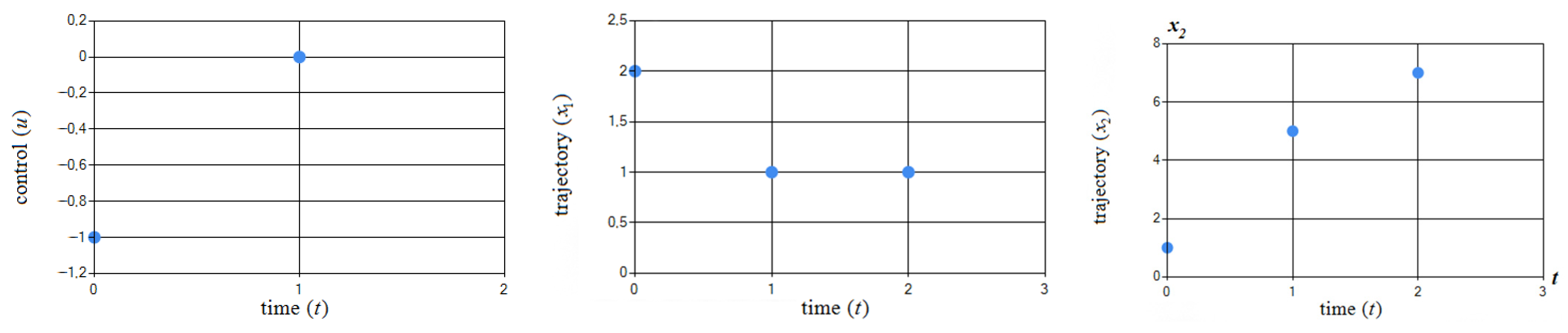
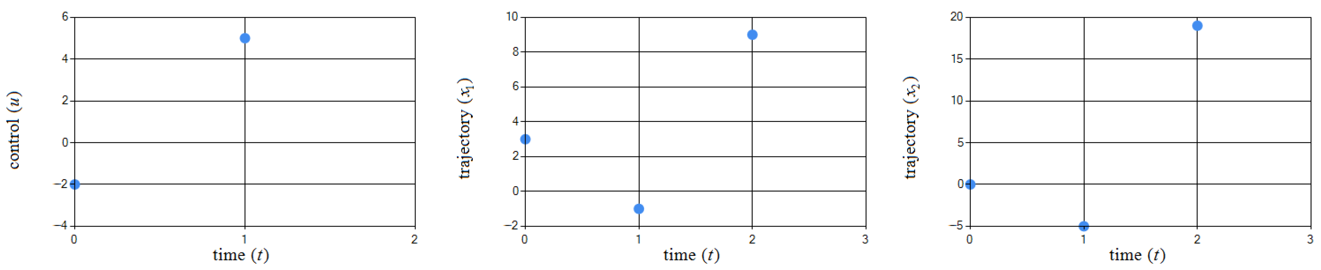
The solution of a stochastic differential equation is a random process, the trajectories of which have sections of continuous change, interrupted by jumps of a given intensity. It describes the movement of the tomtit, accompanied by relatively short jumps. This solution can be found by numerical integration with a step size $h$. If any coordinate value hits the boundary of the search area or goes beyond it, then it is taken equal to the value on this boundary. The best position achieved during the current iteration is chosen as the new position $x^{j,k,search}$ of the tomtit. 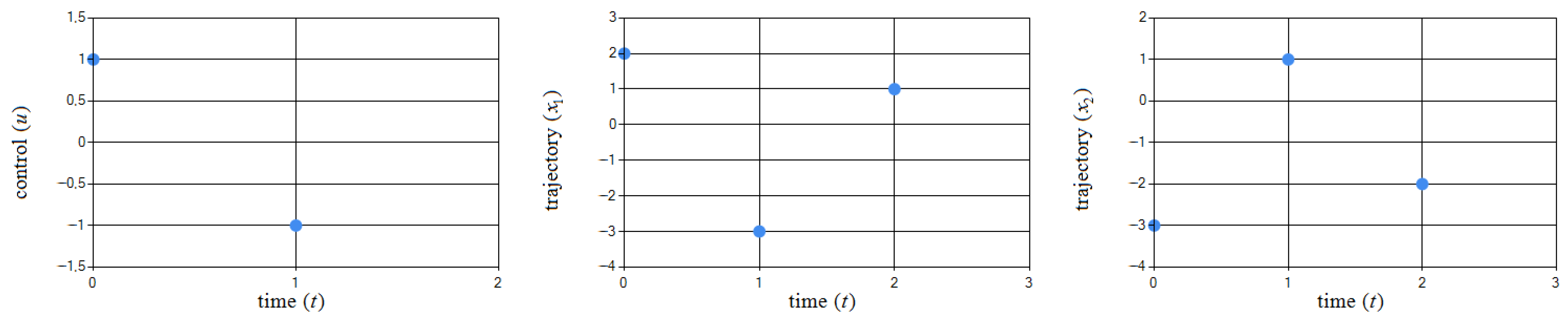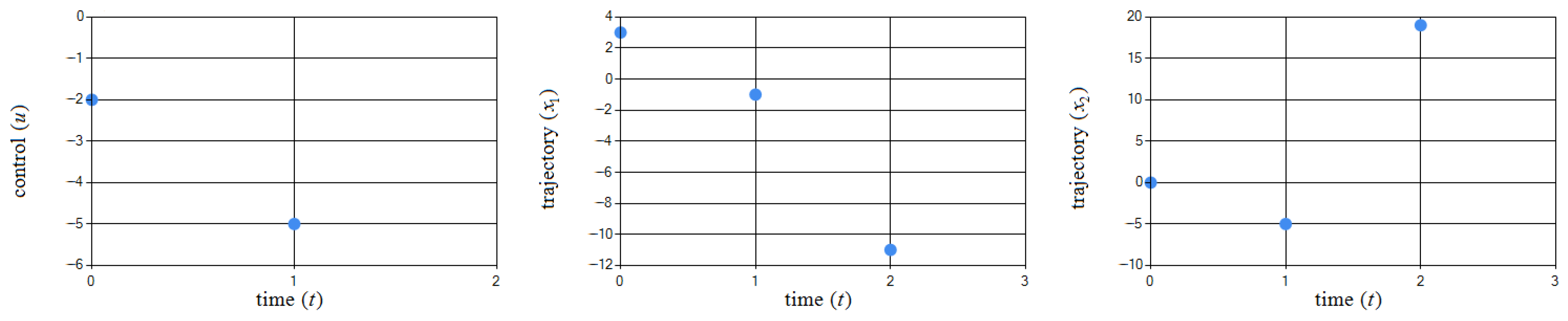This process is shown in Figure 1a. Among all the new positions of tomtits, the best one is selected. It is recorded in the memory matrix and identified with the final position of the leader of the flock at the current iteration, after which the next iteration begins with the procedure for finding a new position of the leader of the flock and the initial positions of the members of the flock relative to it. This procedure is shown in Figure 1b. The method terminates when the maximum number of passes P is reached.

The proposed hybrid method uses the ideas of evolutionary methods to create the initial population [15,16,17,18], the method of imitating the behavior of cuckoo to simulate the jump of the flock leader based on Levy flights [29], the application of a modified numerical Euler–Maruyama method for solving a stochastic differential equation describing the movement of individuals in a population [31]; the idea of particle swarm optimization technique in a flock for describing the interaction of individuals with each other, the modified method of artificial immune systems for updating the population, the Luus-Jaakola method for updating the search set at the end of the next pass [1].

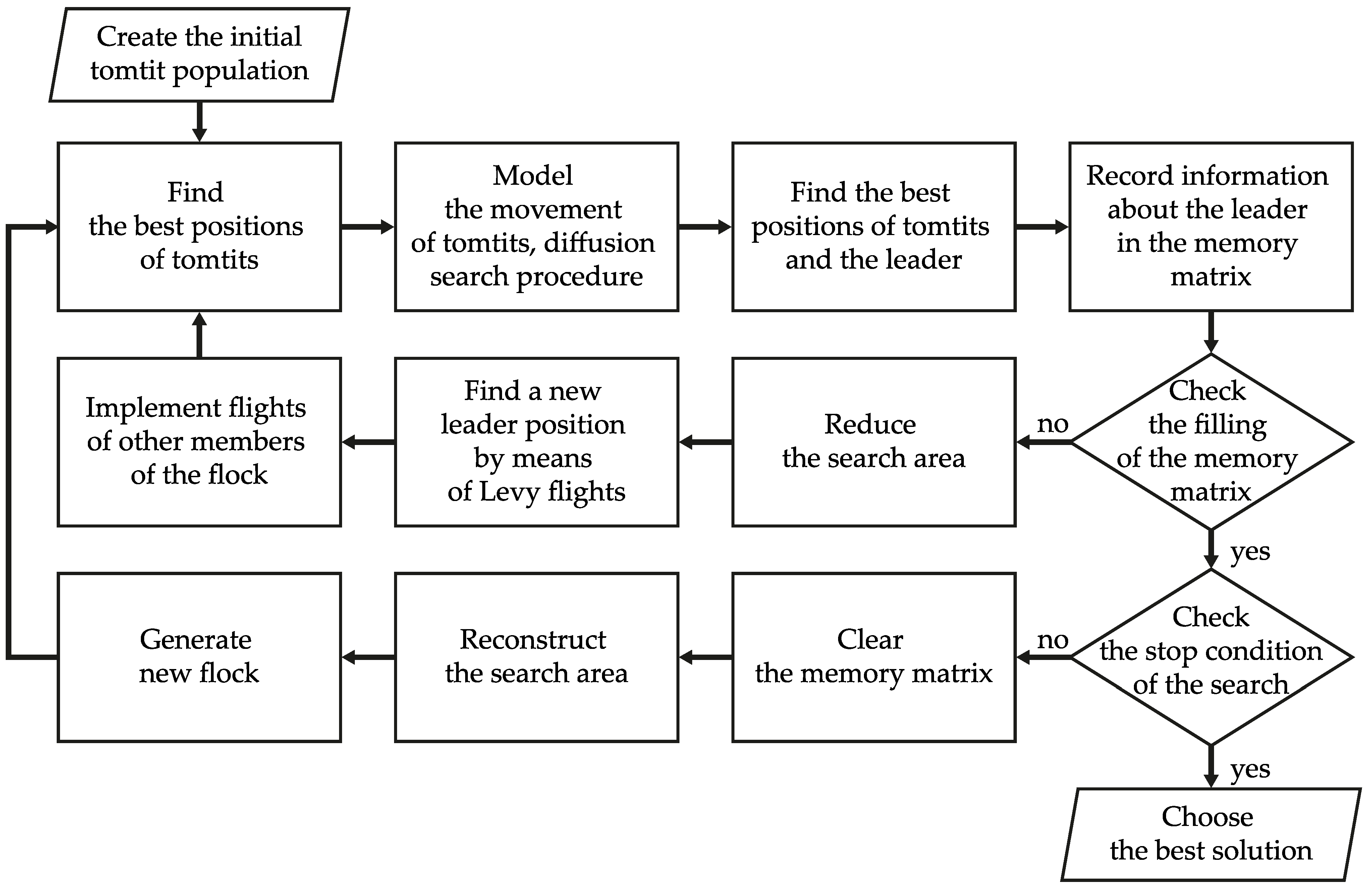
Figure 2 below illustrates the block diagram of the algorithm.

Below is a detailed description of the algorithm.

Step 1. Creation of the initial tomtit population:

Step 1.1. Set parameters of method:

• Number of tomtits in population $NP$;
• Flock leader movement step $\mathsf{\alpha }$;
• Reduction parameter of search set $\mathsf{\gamma }$;
• Reconstruction parameter of search set $\mathsf{\eta }$;
• Levy distribution parameter $\mathsf{\lambda }$;
• Tomtit’s neighborhood radius size $\mathsf{\rho }$;
• Parameters $c_1$, $c_2$, $c_3$, which describe drift vector and diffusion matrix in the stochastic differential equation;
• Number of maximum records in memory matrix $K$;
• Integration step size $h$;
• Number of maximum discrete steps $L$;
• Time required for searching by tomtits $T_t=Lh$;
• Number of maximum passes $P$;
• Jump intensity parameter $\mathsf{\mu }$.

Set the value $p=0$ (the number of passes), $r^0=1$.

Step 1.2. Create initial population $I=\{x^j={(x_1^j,x_2^j,\dots ,x_n^j)}^T,j=1,2,\dots ,NP\}\subset D$ of $NP$ solutions (tomtits) with randomly generated coordinates $x_i$ from the segment $\left[a_i,b_i\right]$ using a uniform distribution:

$$x_i^j=a_i+ran{d}_i\left[0, 1\right]\cdot \left(b_i-a_i\right),i=1,\dots ,n;\hspace{0.17em}\hspace{0.17em}j=1,\dots ,NP,$$

where $ran{d}_i[0,1]$ is the uniform distribution law on the segment $[0;1]$.

Step 2. Movement of flock members. Implementation of the diffusion search procedure with jumps.

Step 2.1. Set the value: $k=0$ (iteration counter).

Step 2.2. For each member of flock calculate the value of objective function: $f(x^{1,k}),\dots ,f(x^{NP,k})$. Order flock members in increasing (nondecreasing) objective function values. The solution $x^{1,k}$ corresponds to the best value, i.e., the position of the leader.

Step 2.3. Process current information about flock members.

For $j=1$ set the following. The best position is $x^{best}=x^{1,k}$ and the corresponding value of objective function $f(x^{best})=f(x^{1,k})$ in population.

For all other flock members $(j=2,\dots ,NP)$ find:

• The best position of a tomtit $x^{j,best}$ during all iterations and the corresponding value of objective function $f(x^{j,best})$;
• The best position $x^{j,local}$ among all tomtits located in the vicinity of the $j$-th individual of radius $\mathsf{\rho }$ and the corresponding value of objective function $f(x^{j,local})$.

Step 2.4. For each $j=2,\dots ,NP$ find the numerical solution of the stochastic differential equation with step size $h$ on the segment $[0,Lh]$ using the Euler–Maruyama method.

Step 2.4.1. Set the value: $x^{j,k}(0)=x^{j,k}$ and $l=0$.

Step 2.4.2. Find the diffusion part of the solution

$${\tilde{x}}^{j,k}(l+1)=x^{j,k}(l)+h\mathit{f}(x^{j,k}(l))+\sqrt{h}\mathsf{\sigma }(x^{j,k}(l))\xi ,$$

where

$$\begin{gathered} \mathit{f}(x^{j,k}(l))=c_1\hspace{0.17em}{r}_1\hspace{0.17em}[x^{best}-x^{j,k}(l)], \\ \mathsf{\sigma }(x^{j,k}(l))=c_2{r}_2[x^{j,best}-x^{j,k}(l)]+c_3{r}_3[x^{j,local}-x^{j,k}(l)], \end{gathered}$$

$r_1,r_2,r_3$ are random parameters uniformly distributed on the segment $[0,1]$ and $\mathsf{\xi }$ is a random variable that has a standard normal distribution with zero mean value and unit variance value. It is possible to model this variable using the Box–Muller method:

$$\mathsf{\xi }=\sqrt{-2\ln {\mathsf{\alpha }}_1}\cos 2\mathsf{\pi }{\mathsf{\alpha }}_2 \mathrm{or} \mathsf{\xi }=\sqrt{-2\ln {\mathsf{\alpha }}_1}\sin 2\mathsf{\pi }{\mathsf{\alpha }}_2,$$

in which ${\mathsf{\alpha }}_1$ and ${\mathsf{\alpha }}_2$ are an independent random variables uniformly distributed on the segment $(0;1)$.

Step 2.4.3. Check jump condition: $\mathsf{\beta }\le \mathsf{\mu }h$, where $\mathsf{\beta }$ is a random variable uniformly distributed on the segment $(0;1)$. In the process of integration, one should check whether the solution belongs to the set of feasible solutions: if any coordinate value of the solution hits the boundary of the search area or goes beyond it, then it is taken equal to the corresponding value on the boundary.

If the jump condition is satisfied, then set the value:

$$x_{}^{j,k}(l+1)={\tilde{x}}_{}^{j,k}(l+1)+\mathsf{\theta },$$

where $\mathsf{\theta }$ is a random increment, in which coordinates are modeled according to the uniform distribution law: ${\mathsf{\theta }}_i\in [-{\Delta }_i,{\Delta }_i],$ ${\Delta }_i=\min [(b_i-{\tilde{x}}_i^{j,k}(l+1),({\tilde{x}}_i^{j,k}(l+1)-a_i)]$.

Otherwise, set the value: $x_{}^{j,k}(l+1)={\tilde{x}}_{}^{j,k}(l+1).$

Step 2.4.4. Check the stop condition of the moving process of a flock’s member.

If $l<L$, set the value $l=l+1$ and go to step 2.4.2. Otherwise, go to step 2.5.

Step 2.5. For each flock member ($j=2,\dots ,NP$), find the best solution among all solutions obtained: $x^{j,k}(0),x^{j,k}(1),\dots ,x^{j,k}(L)$. Denote it as $x^{j,k,search},\hspace{0.17em}\hspace{0.17em}\hspace{0.17em}j=2,\dots ,NP$.

Step 2.6. Among positions $x^{1,k},x^{2,k,search},\dots ,x^{NP,k,search}$ of tomtits (solutions) find the best one. Record it in the memory matrix. This is the leader’s position at the end of the current iteration $x^{1,k,search}$.

Step 2.7. Check the stop condition of a pass. If $k=K$(memory matrix is full) or $r^k<\mathsf{\epsilon }$, then stop the pass. From the memory matrix, choose the best solution and put it in the set Pool, then go to step 3. If $k<K$, set the value $r^{k+1}=\mathsf{\gamma }{r}^k$, $k=k+1$ and go to step 2.8.

Step 2.8. Find the new position of the leader:

$$x^{1,k}=x^{1,k,search}+\frac{\mathsf{\alpha }}{k+1}Levy(\mathsf{\lambda }).$$

To generate a random variable according to the Levy distribution, it is required: for each coordinate $x_i=Lev{y}_i(\mathsf{\lambda })$ to generate number $R_i$, $i=1,\dots ,n$ by uniform distribution law on the set $\left[\mathsf{\epsilon };\hspace{0.17em}\hspace{0.17em}{b}_i-a_i\right],$ where $\mathsf{\epsilon }={10}^{-7}-$ distinguishability constant, and carry out the following [10]:

• Generate numbers ${\mathsf{\theta }}_i=R\cdot i2\mathsf{\pi }$ and $L_i={\left(R_i+\mathsf{\epsilon }\right)}^{-\hspace{0.17em}\hspace{0.17em}\frac{1}{\mathsf{\lambda }}}$, $i=1,\dots ,n$, where $\mathsf{\lambda }$ is a distribution parameter;
• Calculate values of coordinates:

  $$x_i(\mathsf{\lambda })=L_i\sin {\mathsf{\theta }}_i, i=1,\dots ,\left[\frac{n}{2}\right]; x_i(\mathsf{\lambda })=L_i\cos {\mathsf{\theta }}_i, i=\left[\frac{n}{2}\right]+1,\dots ,n.$$

If the obtained value of the coordinate $x_i$ does not belong to the set of feasible solutions; that is $x_i\notin [a_i;b_i]$, then repeat the generation process for the coordinate $x_i$.

If, after ten unsuccessful generations, the coordinate $x_i$ does not belong to the set of feasible solutions, then generate $x_i$ by uniform distribution law on the set $\left[a_i;b_i\right]$.

Step 2.9. Release the flight of the rest of the tomtits.

Positions of all other tomtits ($j=2,\dots ,NP$) are modeled using a uniform distribution on the parallelepiped set (see step 1.2). The center of the parallelepiped set is determined by the position of the leader of the flock $x^{1,k}$ (see step 2.8), and the lengths of the sides are equal $r^k(b_i-a_i)$, $i=1,\dots ,n$.

If the value of tomtit’s coordinate does not belong to the set of feasible solutions, then generate a new position using uniform distribution:

• On the set $\left[a_i,x_i^{1,k}\right]$ when $x_i^{j,k}<a_i,$ $j=2,\dots ,NP$;
• On the set $\left[x_i^{1,k},b_i\right]$ when $x_i^{j,k}>b_i,$ $j=2,\dots ,NP$.

Go to step 2.2.

Step 3. Check the stop condition of the search. If $p=P$, then stop the process and go to step 4. If $p<P$, clear the memory matrix, increase the counter of passes: $p=p+1$, and set the value $r^0={\mathsf{\eta }}^p$, where $\mathsf{\eta }$ is a reconstruction parameter of the search set.

Generate a new flock of tomtits. Choose the best solution from Pool set: $x^{1,0}$. Positions of all other tomtits ($j=2,\dots ,NP$) are modeled using a uniform distribution on the parallelepiped set (see step 1.2). The center of the parallelepiped set is determined by the position of the leader of the flock $x^{1,0}$, and the lengths of the sides are equal $r^0(b_i-a_i)$, $i=1,\dots ,n$.

If the value of the tomtit’s coordinate does not belong to the set of feasible solutions, then generate a new position using uniform distribution:

• On the set $\left[a_i,x_i^{1,0}\right]$ when $x_i^{j,k}<a_i,$ $j=2,\dots ,NP$;
• On the set $\left[x_i^{1,0},b_i\right]$ when $x_i^{j,k}>b_i,$ $j=2,\dots ,NP$.

Go to step 2.

Step 4. Choosing the best solution. Among solutions in the set $Pool$, find the best one, which is considered to be the approximate solution of the optimization problem.

As a result of generalizing the data obtained both in solving classical separable and nonclassical nonseparable optimal control problems, recommendations for choosing the values of hyperparameters were developed: number of tomtits in population $NP\in \left[10;1000\right]$; flock leader movement step $\mathsf{\alpha }\in \left[0.0001;0.2\right]$; reduction parameter of search set $\mathsf{\gamma }\in \left[0.1;0.99\right]$; reconstruction parameter of search set $\mathsf{\eta }\in \left[0.1;0.9\right]$; Levy distribution parameter $\mathsf{\lambda }\in \left[1.1;2\right]$; tomtit’s neighborhood radius size $\mathsf{\rho }\in \left[1;1000\right]$; parameters $c_1$, $c_2$, $c_3\in \left[0.5;30\right]$; number of maximum records in memory matrix $K\in \left[5;50\right]$; integration step size $h\in \left[0.01;0.1\right]$; number of maximum discrete steps $L\in \left[2;10\right]$; number of maximum passes $P\in \left[10;200\right]$; jump intensity parameter $\mathsf{\mu }\in \left[1;30\right]$.

3. Results

3.1. Example 1. The One-Dimensional Optimal Control Problem with an Exact Solution

The dynamical system is described by the state equation:

$$\hspace{0.17em}\hspace{0.17em}x(t+1)=x(t)+u(t),$$

where $x\in R;\hspace{0.17em}\hspace{0.17em}t=0,1,\dots ,N-1;\hspace{0.17em}\hspace{0.17em}u\in R.$ All variables, i.e., the coordinates of the state vector of dynamical systems and the coordinates of the control vector, hereinafter, are written in the normalized form.

It is required to find such a pair of trajectory and control $\left(x^{*}(\cdot ),\hspace{0.17em}\hspace{0.17em}{u}^{*}(\cdot )\right)$ that the value of the performance index $I$ is minimal:

$$\begin{array}{ccc}I=\frac{1}{2}{\displaystyle \sum _{t=0}^{N-1}{\mathsf{\gamma }}^{-t}{u}^2(t)+x(N)},& & \mathsf{\gamma }>1\end{array}.$$

In this case, it is possible to solve this problem analytically:

$$\begin{array}{ccc}{u}^{*}(t)=-{\mathsf{\gamma }}^t;\hspace{0.17em}& x^{*}(t)=x_0+\frac{\left(1-{\mathsf{\gamma }}^k\right)}{\mathsf{\gamma }-1};\hspace{0.17em}& \min I=x_0+\frac{1-{\mathsf{\gamma }}^N}{2\left(\mathsf{\gamma }-1\right)}.\end{array}$$

In this problem, the initial condition is known: $x(0)=0$, and the constraints on the control are also given: $-2\cdot {10}^4\le u\le 2\cdot {10}^4$. For this task, the number of stages is set: $N=50$; the exact value of the performance index is $\min I=-581.954264398477.$

To solve the problems under consideration with the help of the new TFO algorithm, a computer with the following characteristics was used: an Intel Core i7-2860QM processor with a clock frequency of 3.3 GHz, 16 gigabytes of RAM. To implement the software package, the C# programming language (7.2) with Microsoft Framework. Net version 4.7.2 was used from https://dotnet.microsoft.com/en-us/ (accessed on 25 August 2022).

When solving this problem, the approximate value of the performance index obtained by the TFO algorithm was $I_{TFO}^{*}=-581.953556374572$ and the runtime was 1:07 min. The relative error of the obtained value of the performance index was $1.2\times {10}^{-6}$. The same problem was solved by Perch School Search algorithm [10]. The runtime was 5:36 min and the value of performance index was $I_{PSS}^{*}=-581.954264313551$. It is obvious that the new TFO algorithm makes it possible to obtain solutions much faster and with sufficient accuracy.

To solve this problem, the TFO algorithm was used with the parameters shown in

Table 1. The set of parameters of the TFO algorithm in Example 1.

$\mathit{N}\mathit{P}$	$\mathsf{\gamma }$	$\mathsf{\eta }$	$\mathsf{\rho }$	${\mathit{c}}_1$	${\mathit{c}}_2$	${\mathit{c}}_3$	$\mathit{K}$	$\mathit{h}$	$\mathit{L}$	$\mathit{P}$	$\mathsf{\mu }$	$\mathsf{\epsilon }$	$\mathsf{\lambda }$	$\mathsf{\alpha }$
1000	0.1	0.6	1000	30	30	30	50	0.01	4	160	30	$1\times {10}^{-9}$	1.3	0.1

. Figure 3 shows the obtained pair $\left(x(\cdot ),\hspace{0.17em}\hspace{0.17em}u(\cdot )\right)$.

In order to analyze the effect of algorithm parameters on the result obtained, the same problem was solved with another set of algorithm parameters, which are presented in

Table 2. The set of parameters of the TFO algorithm in Example 1.

$\mathit{N}\mathit{P}$	$\mathsf{\gamma }$	$\mathsf{\eta }$	$\mathsf{\rho }$	${\mathit{c}}_1$	${\mathit{c}}_2$	${\mathit{c}}_3$	$\mathit{K}$	$\mathit{h}$	$\mathit{L}$	$\mathit{P}$	$\mathsf{\mu }$	$\mathsf{\epsilon }$	$\mathsf{\lambda }$	$\mathsf{\alpha }$
1000	0.3	0.6	1000	30	30	30	10	0.01	2	20	30	$1\times {10}^{-9}$	1.3	0.1

. Figure 4 shows the obtained pair $\left(x(\cdot ),\hspace{0.17em}\hspace{0.17em}u(\cdot )\right)$.

The approximate value of the performance index obtained by the TFO algorithm was $I^{*}=-579.311903151533$, and the runtime was 14.92 s. It turned out that the resulting value of the performance index was worse due to other parameters, but the change in relative error was not significant. This example shows the importance of selecting parameters, which is a rather difficult task. A slight change in the parameters can significantly affect the result of solving the problem.

To demonstrate the increase in the runtime to solve the problem, a search for optimal control and the trajectory with the parameters of the algorithm from Table 1 is performed. The difference will be an increase in the number of stages: $N=80$, but the parameters of the system remain unchanged.

Figure 5 shows the obtained pair $\left(x(\cdot ),\hspace{0.17em}\hspace{0.17em}u(\cdot )\right)$.

The exact value of the performance index was $\min I=-10237.001072927329.$ The obtained value of the performance index was $I^{*}=-10174.6684936038$, with a runtime of 1:58 min.

Example 1 illustrates the possibilities of the method in solving financial optimization problems that take the discounting effect into account.

3.2. Example 2. Luus–Tassone Nonseparable Control Problem

The dynamical system is described by three difference equations:

$$\begin{array}{l}{x}_1(t+1)=\frac{x_1(t)}{1+0.01u_1(t)(3+u_2(t))};\hspace{0.17em}\hspace{0.17em}\hspace{0.17em}\\ x_2(t+1)=\frac{x_2(t)+u_1(t)x_1(t+1)}{1+u_1(t)(1+u_2(t))};\hspace{0.17em}\hspace{0.17em}\hspace{0.17em}\\ x_3(t+1)=\frac{x_3(t)}{1+0.01u_2(t)(1+u_3(t))},\end{array}$$

where $\hspace{0.17em}x\in R^3$, $t=0,\dots ,N-1$, and $\hspace{0.17em}u\in R^3$.

It is required to find such a pair of trajectories and control $\left(x^{*}(\cdot ),\hspace{0.17em}\hspace{0.17em}{u}^{*}(\cdot )\right)$ so that the value of the performance index I is minimal:

$$\begin{array}{l}\hspace{0.17em}\hspace{0.17em}\hspace{0.17em}\hspace{0.17em}\hspace{0.17em}\hspace{0.17em}\hspace{0.17em}\hspace{0.17em}\hspace{0.17em}\hspace{0.17em}\hspace{0.17em}\hspace{0.17em}\hspace{0.17em}\hspace{0.17em}\hspace{0.17em}\hspace{0.17em}\hspace{0.17em}\hspace{0.17em}\hspace{0.17em}\hspace{0.17em}\hspace{0.17em}\hspace{0.17em}\hspace{0.17em}\hspace{0.17em}\hspace{0.17em}\hspace{0.17em}\hspace{0.17em}\hspace{0.17em}\hspace{0.17em}\hspace{0.17em}\hspace{0.17em}\hspace{0.17em}\hspace{0.17em}I=x_1{}^2(N)+x_2^2(N)+x_3^2(N)+\\ +{\left[\left({\displaystyle \sum _{k=1}^N{x}_1^2(k-1)+x_2^2(k-1)}+2u_3^2(k-1)\right)\left({\displaystyle \sum _{k=1}^N{x}_3^2(k-1)+2u_1^2(k-1)}+2u_2^2(k-1)\right)\right]}^{\frac{1}{2}}.\end{array}$$

In this problem, the initial condition: $x(0)={(2;\hspace{0.17em}\hspace{0.17em}5;\hspace{0.17em}\hspace{0.17em}7)}^T$, and the constraints on the control are also given: $0\le u_1(t)\le 4$, $0\le u_2(t)\le 4$, $0\le u_3(t)\le 0.5$. For this task, the number of stages is set: $N=20$.

The best known value of the performance index for this problem was obtained in [1]: $\min I=209.26937$ The approximate value of the performance index obtained by the TFO algorithm was $I_{TFO}^{*}=209.389060601957$, and the runtime was 16.47 s. The same problem was solved by the Perch School Search algorithm [10]. The runtime was 49.92 s, and the value of performance index was $I_{PSS}^{*}=209.429533683522$. It is obvious that the new TFO algorithm makes it possible to obtain the solution much faster. However, the obtained solution of this problem is still not as accurate as that of the author of the problem [1]. It turned out to be extremely difficult to select the parameters for the algorithm for this problem.

To solve this problem, the TFO algorithm was used with the parameters shown in

Table 3. The set of parameters of the TFO algorithm in Example 2.

$\mathit{N}\mathit{P}$	$\mathsf{\gamma }$	$\mathsf{\eta }$	$\mathsf{\rho }$	${\mathit{c}}_1$	${\mathit{c}}_2$	${\mathit{c}}_3$	$\mathit{K}$	$\mathit{h}$	$\mathit{L}$	$\mathit{P}$	$\mathsf{\mu }$	$\mathsf{\epsilon }$	$\mathsf{\lambda }$	$\mathsf{\alpha }$
300	0.3	0.9	2	2	0.5	3	10	0.05	10	100	1	$1\times {10}^{-9}$	1.1	0.0001

. Figure 6 and Figure 7 show the obtained pair $\left(x(\cdot ),\hspace{0.17em}\hspace{0.17em}u(\cdot )\right)$.

3.3. Example 3. Li–Haimes Nonseparable Control Problem

The dynamical system is described by three difference equations:

$$\begin{array}{ccc}x(1)=x{(0)}^{u(0)};& x(2)=(1+u(1))\cdot x(1);& x(3)=x(2)+u(2),\end{array}$$

where $x\in R$, $t=0,1,2$, and $u\in R$.

It is required to find such a pair of trajectory and control $\left(x^{*}(\cdot ),\hspace{0.17em}\hspace{0.17em}{u}^{*}(\cdot )\right)$ that the value of the performance index $I$ is minimal:

$$I=[x^2(0)+x^2(1)+(2x^2(2)+x^2(3))\exp (x^2(1))]\times \hspace{0.17em}{[50+u^2(0)+(u^2(1)+u^2(2))\exp (u^2(0))]}^{1/2}.$$

In this problem, the initial condition is known: $x(0)=15$, and the constraints on the control are also given: $-1\le u(t)\le 1$, $t=0,1,2$. For this task, the number of stages is set: $N=3$. The best-known value of the performance index obtained for this nonseparable control problem was obtained in [1]: $\min I=1596.4796778$.

The approximate value of the performance index obtained by the TFO algorithm was $I_{TFO}^{*}=1596.47967783381$ and the runtime was 0.13 s. The same problem was solved by Perch School Search algorithm [10]. The runtime was 0.19 s and the value of performance index was $I_{PSS}^{*}=1596.47967783389$. The new TFO algorithm makes it possible to obtain almost the same solution much faster.

To solve this problem, the TFO algorithm was used with the parameters shown in

Table 4. The set of parameters of the TFO algorithm in Example 3.

$\mathit{N}\mathit{P}$	$\mathsf{\gamma }$	$\mathsf{\eta }$	$\mathsf{\rho }$	${\mathit{c}}_1$	${\mathit{c}}_2$	${\mathit{c}}_3$	$\mathit{K}$	$\mathit{h}$	$\mathit{L}$	$\mathit{P}$	$\mathsf{\mu }$	$\mathsf{\epsilon }$	$\mathsf{\lambda }$	$\mathsf{\alpha }$
100	0.1	0.1	5	3	3	3	10	0.1	5	100	2	$1\times {10}^{-9}$	1.5	0.001

. Figure 8 shows the obtained pair $\left(x(\cdot ),\hspace{0.17em}\hspace{0.17em}u(\cdot )\right)$. The values of the obtained control $u(\cdot )$ and trajectory $x(\cdot )$ are shown in

Table 5. The values of the obtained control and trajectory.

$\mathit{t}$	$\mathit{u}$	$\mathit{x}$
0	−0.42716	15
1	−0.09897	0.31450
2	−0.08238	0.28337
3		0.20099

.

Examples 2 and 3 illustrate the possibilities of solving complex optimal control problems with nonseparable performance indexes, for which obtaining solutions using known optimality conditions is extremely difficult.

3.4. Example 4. The Two-Dimensional Lagrange Optimal Control Problem with an Exact Solution

The dynamical system is described by two difference equations:

$$\begin{array}{ll}{x}_1(t+1)=x_1(t)+u(t);\hfill & x_2(t+1)=2x_1(t)+x_2(t),\hfill \end{array}$$

where $x\in R^2$, $t=0,1$, and $u\in R$.

It is required to find such a pair of trajectory and control $\left(x^{*}(\cdot ),\hspace{0.17em}\hspace{0.17em}{u}^{*}(\cdot )\right)$ that the value of the performance index $I$ is minimal:

$$I={\displaystyle \sum _{t=0}^1\left[x_1{}^2(t)+x_2^2(t)+u^2(t)\right]}\hspace{0.17em}.$$

In this problem, the initial condition $x(0)={(2;1)}^T$ and the constraints on the control are also given: $-{10}^5\le u\le {10}^5$, the number of stages is set: $N=2$. The exact value of the performance index is $\min I=32.$ For this control problem, the analytical solution can be found: ${\mathit{u}}^{*}=\{-1;0\}$; ${\mathit{x}}_1^{*}(\cdot )=\{2;1;1\}$; ${\mathit{x}}_2^{*}(\cdot )=\{1;5;7\}$.

The approximate value of the performance index obtained by the TFO algorithm was $I_{TFO}^{*}=32.0000000000001$ and the runtime was less than 0.01 s. The relative error of the obtained value of the performance index was $3.1\times {10}^{-15}$. The same problem was solved by the Perch School Search algorithm [10]. The runtime was 1.58 s and the value of the performance index was $I_{PSS}^{*}=32$. The new TFO algorithm makes it possible to obtain solutions much faster and with almost the same accuracy.

To solve this problem, the TFO algorithm was used with the parameters shown in

Table 6. The set of parameters of the TFO algorithm in Example 4.

$\mathit{N}\mathit{P}$	$\mathsf{\gamma }$	$\mathsf{\eta }$	$\mathsf{\rho }$	${\mathit{c}}_1$	${\mathit{c}}_2$	${\mathit{c}}_3$	$\mathit{K}$	$\mathit{h}$	$\mathit{L}$	$\mathit{P}$	$\mathsf{\mu }$	$\mathsf{\epsilon }$	$\mathsf{\lambda }$	$\mathsf{\alpha }$
70	0.1	0.1	100	2	3	2	5	0.1	6	10	2	$1\times {10}^{-9}$	1.5	0.001

. Figure 9 shows the obtained pair $\left(x(\cdot ),\hspace{0.17em}\hspace{0.17em}u(\cdot )\right)$.

3.5. Example 5. The Two-Dimensional Meyer Optimal Control Problem with an Exact Solution

The dynamical system is described by two difference equations:

$$\begin{array}{ll}{x}_1(t+1)=x_1(t)+u(t);\hfill & x_2(t+1)=2x_1(t)+x_2(t),\hfill \end{array}$$

where $x\in R^2$, $t=0,1$, and $u\in R$.

It is required to find such a pair of trajectory and control $\left(x^{*}(\cdot ),\hspace{0.17em}\hspace{0.17em}{u}^{*}(\cdot )\right)$ that the value of the performance index $I$ is minimal:

$$I=x_1^2(2)+x_2^2(2).$$

In this problem, the initial condition vector is known: $x(0)={(2;-3)}^T$, and the constraints on the control are also given: $-1\le u\le 1$. For this task, the number of stages is set: $N=2$; the exact value of the performance index is $\min I=5.$

The approximate value of the performance index obtained by the TFO algorithm was $I_{TFO}^{*}=5$ and the runtime was less than 0.01 s. The same problem was solved by Perch School Search algorithm [10]. The runtime was 0.25 s and the value of the performance index was $I_{PSS}^{*}=5.00000000000002.\mathrm{}$. It is obvious that the new TFO algorithm makes it possible to obtain the solution much faster and with almost the same accuracy.

To solve this problem, the TFO algorithm was used with the parameters shown in

Table 7. The set of parameters of the TFO algorithm in Example 5.

$\mathit{N}\mathit{P}$	$\mathit{\gamma }$	$\mathsf{\eta }$	$\mathsf{\rho }$	${\mathit{c}}_1$	${\mathit{c}}_2$	${\mathit{c}}_3$	$\mathit{K}$	$\mathit{h}$	$\mathit{L}$	$\mathit{P}$	$\mathsf{\mu }$	$\mathsf{\epsilon }$	$\mathsf{\lambda }$	$\mathsf{\alpha }$
30	0.81	0.6	2	1	1	1	5	0.1	6	10	2	$1\times {10}^{-9}$	1.2	0.2

. Figure 10 shows the obtained pair $\left(x(\cdot ),\hspace{0.17em}\hspace{0.17em}u(\cdot )\right)$. The values of the obtained control and trajectory components are shown in

Table 8. The values of the obtained control and trajectory.

$\mathit{t}$	$\mathit{u}$	${\mathit{x}}_1$	${\mathit{x}}_2$
0	1	2	−3
1	−1	−3	1
2		1	−2

.

Examples 4 and 5 illustrate the possibility of solving the problem of finding the optimal program control for classical control problems for linear discrete deterministic dynamical systems with a quadratic performance index.

3.6. Example 6. The Two-Dimensional Bolza Optimal Control Problem with an Exact Solution

The dynamical system is described by two difference equations:

$$\begin{array}{ll}{x}_1(t+1)=x_2(t);\hfill & x_2(t+1)=2x_2(t)-x_1(t)+\frac{1}{N^2}u(t),\hfill \end{array}$$

where $x\in R^2$, $t=0,1,\dots ,N-1$, and $u\in R$.

It is required to find such a pair of trajectory and control $\left(x^{*}(\cdot ),\hspace{0.17em}\hspace{0.17em}{u}^{*}(\cdot )\right)$ that the value of the performance index $I$ is minimal:

$$I=-x_1(N)+\frac{1}{2N}{\displaystyle \sum _{t=0}^{N-1}{u}^2(t)}.$$

In this case, it is possible to solve this problem analytically:

$$\begin{array}{cc}{u}^{*}(t)=\frac{N-t-1}{N};& \min I=-\frac{1}{3}+\frac{3N-1}{6N^2}+\frac{1}{2N^3}{\displaystyle \sum _{t=0}^{N-1}{t}^2}.\end{array}$$

In this problem, the initial condition vector is known: $x(0)={(0;0)}^T$, and the constraints on the control are also given: $0\le u\le 100$. For this task, the number of stages is set: $N=10.$; the exact value of the performance index is $\min I=-0.1425.$

When solving this problem, the approximate value of the performance index obtained by the TFO algorithm was $I_{TFO}^{*}=-0.142499964879453$ and the runtime was 0.13 s. The relative error of the obtained value of the performance index was $2.5\times {10}^{-7}$. The same problem was solved by Perch School Search algorithm [7]. The runtime was 7.39 s and the value of the performance index was $I_{PSS}^{*}=-0.142499999999796$. The new algorithm makes it possible to obtain solutions much faster and with almost the same accuracy.

To solve this problem, the TFO algorithm was used with the parameters shown in

Table 9. The set of parameters of the TFO algorithm in Example 6.

$\mathit{N}\mathit{P}$	$\mathsf{\gamma }$	$\mathsf{\eta }$	$\mathsf{\rho }$	${\mathit{c}}_1$	${\mathit{c}}_2$	${\mathit{c}}_3$	$\mathit{K}$	$\mathit{h}$	$\mathit{L}$	$\mathit{P}$	$\mathsf{\mu }$	$\mathsf{\epsilon }$	$\mathsf{\lambda }$	$\mathsf{\alpha }$
120	0.9	0.2	40	10	10	10	20	0.1	4	20	3	$1\times {10}^{-9}$	1.7	0.1

. Figure 11 shows the obtained pair $\left(x(\cdot ),\hspace{0.17em}\hspace{0.17em}u(\cdot )\right)$. Figure 12 shows deviations of approximate control values from exact ones at different moments of the dynamic system operation, i.e., $\Delta u(t)=\left|u(t)-u*(t)\right|$.

3.7. Example 7. The Two-Dimensional Meyer Optimal Control Problem with an Exact Solution

The dynamical system is described by two difference equations:

$$\begin{array}{ll}{x}_1(t+1)=x_1(t)+2u(t);\hfill & x_2(t+1)=-x_1^2(t)+x_1(t)+u^2(t),\hfill \end{array}$$

where $x\in R^2$, $t=0,1$, and $u\in R$.

It is required to find such a pair of trajectory and control $\left(x^{*}(\cdot ),\hspace{0.17em}\hspace{0.17em}{u}^{*}(\cdot )\right)$ that the value of the performance index $I$ is minimal:

$$I=-x_2(2).$$

In this problem, the initial condition vector is known: $x(0)={(3;0)}^T$, and the constraints on the control are also given: $-5\le u\le 5$. For this task, the number of stages is set: $N=2$; the exact value of the performance index is $\min I=-19.$

In this example, the convex varying condition is not satisfied, which means that the discrete maximum principle cannot be applied, while the necessary optimality conditions are satisfied.

This problem has two solutions: $x_1^{1*}(\cdot )=\left\{3;-1;9\right\}$, $x_2^{1*}(\cdot )=\left\{0;-5;19\right\}$, $u^{1*}(\cdot )=\left\{-2;5\right\}$ and $x_1^{2*}(\cdot )=\left\{3;-1;-11\right\}$, $x_2^{2*}(\cdot )=\left\{0;-5;19\right\}$, $u^{2*}(\cdot )=\left\{-2;-5\right\}$; the TFO algorithm successfully finds both solutions.

When solving this problem, the approximate values of the performance index obtained by the TFO algorithm for both solutions were: $I_{TFO}^{1*}=-18.999999999918$ (the runtime was less than 0.01 s for the first solution); $I_{TFO}^{2*}=-18.9999999991551$(the runtime was less than 0.01 s for the second solution). The relative errors of the obtained value of the performance index were $4.3\times {10}^{-12}$ and $4.4\times {10}^{-11}$, respectively. The same problem was solved by the Perch School Search algorithm [7]. Runtimes were 0.30 s and 0.31 s, and the values of the performance index were $I_{PSS}^{1*}=-18.9999999999354$ and $I_{PSS}^{2*}=-18.9999999999939$, respectively. The TFO algorithm makes it possible to obtain solutions much faster and with almost the same accuracy.

To solve this problem, the TFO algorithm was used with the parameters shown in

Table 10. The set of parameters of the TFO algorithm in Example 7.

$\mathit{N}\mathit{P}$	$\mathsf{\gamma }$	$\mathsf{\eta }$	$\mathsf{\rho }$	${\mathit{c}}_1$	${\mathit{c}}_2$	${\mathit{c}}_3$	$\mathit{K}$	$\mathit{h}$	$\mathit{L}$	$\mathit{P}$	$\mathsf{\mu }$	$\mathsf{\epsilon }$	$\mathsf{\lambda }$	$\mathsf{\alpha }$
30	0.81	0.4	3	2.5	2.7	2.8	20	0.1	4	30	2.5	$1\times {10}^{-9}$	2	0.01

. Figure 13 and Figure 14 show the obtained pairs $\left(x(\cdot ),\hspace{0.17em}\hspace{0.17em}u(\cdot )\right)$ for both solutions. The values of the obtained control and trajectory components are shown in

Table 11. The values of the obtained control and trajectory components for the first solution.

$\mathit{t}$	$\mathit{u}$	${\mathit{x}}_1$	${\mathit{x}}_2$
0	−2.00001	3	0
1	5	−1.00001	−4.99998
2		8.99999	19

and

Table 12. The values of the obtained control and trajectory components for the second solution.

$\mathit{t}$	$\mathit{u}$	${\mathit{x}}_1$	${\mathit{x}}_2$
0	−1.99998	3	0
1	−5	−0.99997	−5.00007
2		−10.99997	19

.

4. Conclusions

In this paper, a new bio-inspired metaheuristic optimization algorithm named TFO, used to find the solution to open-loop control problems for discrete deterministic dynamical systems, is proposed.

This algorithm has successfully inherited a number of new ideas and known techniques from several algorithms; for example, the numerical solution of stochastic differential equations with jumps by the Euler–Maruyama method to describe the movement of tomtits when foraging, compression and recovery of the search area б exchange of information between members of the flock. These ideas allow the algorithm to solve applied optimization problems in a short runtime, which was shown by examples of the problem of finding optimal control and trajectories of discrete dynamical systems. The solutions obtained in most cases are extremely close, or coincide with the analytical solutions if they are known. Compared to the previously developed PSS algorithm, this algorithm is more efficient when it comes to solving problems of finding the optimal control and trajectory, which is shown by the through comparison of the running time of the algorithm and the relative error.

In the future, we plan to improve this algorithm or create new algorithms based on the TFO algorithm in order to obtain more accurate (but no less fast) algorithms.

The direction of further development of this work can be the application of the developed metaheuristic optimization algorithm in solving applied problems of optimal control of aircraft of various types and optimal control problems with full and incomplete feedback on the measured variables, as well as solving problems in the presence of uncertainty when setting the initial state vector.

References

1. Luus, R. Iterative Dynamic Programming, 1st ed.; Chapman & Hall/CRC: London, UK, 2000. [Google Scholar]
2. Yang, X.S.; Chien, S.F.; Ting, T.O. Bio-Inspired Computation and Optimization, 1st ed.; Morgan Kaufmann: New York, NY, USA, 2015. [Google Scholar]
3. Goldberg, D. Genetic Algorithms in Search, Optimization and Machine Learning, 1st ed.; Addison-Wesley Publishing Company: Boston, MA, USA, 1989. [Google Scholar]
4. Michalewicz, Z.; Fogel, D. How to Solve It: Modern Heuristics, 2nd ed.; Springer: New York, NY, USA, 2004. [Google Scholar]
5. Panteleev, A.V.; Lobanov, A.V. Application of Mini-Batch Metaheuristic algorithms in problems of optimization of deterministic systems with incomplete information about the state vector. Algorithms 2021, 14, 332. [Google Scholar] [CrossRef]
6. Roni, H.K.; Rana, M.S.; Pota, H.R.; Hasan, M.; Hussain, S. Recent trends in bio-inspired meta-heuristic optimization techniques in control applications for electrical systems: A review. Int. J. Dyn. Control. 2022, 10, 999–1011. [Google Scholar] [CrossRef]
7. Floudas, C.A.; Pardalos, P.M.; Adjiman, C.S.; Esposito, W.R.; Gümüs, Z.H.; Harding, S.T.; Klepeis, J.L.; Meyer, C.A.; Schweiger, C.A. Handbook of Test Problems in Local and Global Optimization, 1st ed.; Kluwer Academic Publishers: Dordrecht, The Netherlands, 1999. [Google Scholar]
8. Roman, R.C.; Precup, R.E.; Petriu, E.M. Hybrid data-driven fuzzy active disturbance rejection control for tower crane systems. Eur. J. Control 2021, 58, 373–387. [Google Scholar] [CrossRef]
9. Chi, R.; Li, H.; Shen, D.; Hou, Z.; Huang, B. Enhanced P-type control: Indirect adaptive learning from set-point updates. IEEE Trans. Autom. Control 2022. [Google Scholar] [CrossRef]
10. Panteleev, A.V.; Kolessa, A.A. Optimal open-loop control of discrete deterministic systems by application of the perch school metaheuristic optimization algorithm. Algorithms 2022, 15, 157. [Google Scholar] [CrossRef]
11. Sergeyev, Y.D.; Kvasov, D.E.; Mukhametzhanov, M.S. On the efficiency of nature-inspired metaheuristics in expensive global optimization with limited budget. Sci. Rep. 2018, 8, 453. [Google Scholar] [CrossRef] [PubMed]
12. Sergeyev, Y.D.; Kvasov, D.E. Deterministic Global Optimization: An Introduction to the Diagonal Approach, 1st ed.; Springer: New York, NY, USA, 2017. [Google Scholar]
13. Pinter, J.D. Global Optimization in Action (Continuous and Lipschitz Optimization: Algorithms, Implementations and Applications), 1st ed.; Kluwer Academic Publishers: Dordrecht, The Netherlands, 1996. [Google Scholar]
14. Chambers, D.L. Practical Handbook of Genetic Algorithms, Applications, 2nd ed.; Chapman & Hall/CRC: London, UK, 2001. [Google Scholar]
15. Floudas, C.; Pardalos, P. Encyclopedia of Optimization, 2nd ed.; Springer: New York, NY, USA, 2009. [Google Scholar]
16. Gendreau, M. Handbook of Metaheuristics, 2nd ed.; Springer: New York, NY, USA, 2010. [Google Scholar]
17. Glover, F.W.; Kochenberger, G.A. (Eds.) Handbook of Metaheuristics; Kluwer Academic Publishers: Boston, MA, USA, 2003. [Google Scholar]
18. Neri, F.; Cotta, C.; Moscato, P. Handbook of Memetic Algorithms, 1st ed.; Springer: Berlin/Heidelberg, Germany, 2012. [Google Scholar]
19. Chattopadhyay, S.; Marik, A.; Pramanik, R. A brief overview of physics-inspired metaheuristic optimization techniques. arXiv 2022, arXiv:2201.12810v1. [Google Scholar]
20. Beheshti, Z.; Shamsuddin, S.M. A review of population-based meta-heuristic algorithms. Int. J. Adv. Soft Comput. Appl. 2013, 5, 1–35. [Google Scholar]
21. Locatelli, M.; Schoen, F. (Global) Optimization: Historical notes and recent developments. EURO J. Comput. Optim. 2021, 9, 100012. [Google Scholar] [CrossRef]
22. Dragoi, E.N.; Dafinescu, V. Review of metaheuristics inspired from the animal kingdom. Mathematics 2021, 9, 2335. [Google Scholar] [CrossRef]
23. Brownlee, J. Clever Algorithms: Nature-Inspired Programming Recipes, 1st ed.; LuLu.com: Raleigh, CA, USA, 2011. [Google Scholar]
24. Tzanetos, A.; Fister, I.; Dounias, G. A comprehensive database of nature-inspired algorithms. Data Brief 2020, 31, 105792. [Google Scholar] [CrossRef] [PubMed]
25. Fister, I., Jr.; Yang, X.-S.; Fister, I.; Brest, J.; Fister, D. A brief review of nature-inspired algorithms for optimization. arXiv 2013, arXiv:1307.4186. [Google Scholar]
26. Yang, X.S. Nature-Inspired Metaheuristic Algorithms, 2nd ed.; Luniver Press: Frome, UK, 2010. [Google Scholar]
27. Panteleev, A.V.; Belyakov, I.A.; Kolessa, A.A. Comparative analysis of optimization strategies by software complex “Metaheuristic nature-inspired methods of global optimization”. J. Phys. Conf. Ser. 2022, 2308, 012002. [Google Scholar] [CrossRef]
28. Del Ser, J.; Osaba, E.; Molina, D.; Yang, X.-S.; Salcedo-Sanz, S.; Camacho, D.; Das, S.; Suganthan, P.N.; Coello Coello, C.A.; Herrera, F. Bio-inspired computation: Where we stand and what’s next. Swarm Evol. Comput. 2019, 48, 220–250. [Google Scholar] [CrossRef]
29. Yang, X.S.; Deb, S. Cuckoo search via Levy flights. In Proceedings of World Congress on Nature and Biologically Inspired Computing, Coimbatore, India, 9–11 December 2009; pp. 210–214. [Google Scholar]
30. Wolpert, D.H.; Macready, W.G. No free lunch theorems for optimization. IEEE Trans. Evolut. Comput. 1997, 1, 67–82. [Google Scholar] [CrossRef] [Green Version]
31. Averina, T.A.; Rybakov, K.A. Maximum cross section method in optimal filtering of jump-diffusion random processes. In Proceedings of the 15th International Asian School-Seminar Optimization Problems of Complex Systems, Novosibirsk, Russia, 26–30 August 2019; pp. 8–11. [Google Scholar]
Figure 1. Movement of tomtits; (a) stochastic movement of tomtits, choosing the best solution and adding into the memory matrix, (b) new position of the leader and flight results of other tomtits.
Algorithms 15 00301 g001
Figure 2. A block diagram of the proposed TFO algorithm.
Algorithms 15 00301 g002
Figure 3. Graphical illustration of obtained pair ( x ( ) , u ( ) ) in Example 1.
Algorithms 15 00301 g003
Figure 4. Graphical illustration of obtained pair ( x ( ) , u ( ) ) in Example 1.
Algorithms 15 00301 g004
Figure 5. Graphical illustration of obtained pair ( x ( ) , u ( ) ) in Example 1.
Algorithms 15 00301 g005
Figure 6. Graphical illustration of obtained u ( ) in Example 2.
Algorithms 15 00301 g006
Figure 7. Graphical illustration of obtained x ( ) in Example 2.
Algorithms 15 00301 g007
Figure 8. Graphical illustration of obtained pair ( x ( ) , u ( ) ) in Example 3.
Algorithms 15 00301 g008
Figure 9. Graphical illustration of obtained pair ( x ( ) , u ( ) ) in Example 4.
Algorithms 15 00301 g009
Figure 10. Graphical illustration of obtained pair ( x ( ) , u ( ) ) in Example 5.
Algorithms 15 00301 g010
Figure 11. Graphical illustration of obtained pair ( x ( ) , u ( ) ) in Example 6.
Algorithms 15 00301 g011
Figure 12. Deviations of approximate control values from the exact ones.
Algorithms 15 00301 g012
Figure 13. Graphical illustration of obtained pair ( x ( ) , u ( ) ) for the first solution in Example 7.
Algorithms 15 00301 g013
Figure 14. Graphical illustration of obtained pair ( x ( ) , u ( ) ) for the second solution in Example 7.
Algorithms 15 00301 g014