Article

Boosting the Performance of CDCL-Based SAT Solvers by Exploiting Backbones and Backdoors

by
Tasniem Al-Yahya
*,
Mohamed El Bachir Abdelkrim Menai
and
Hassan Mathkour
Department of Computer Science, College of Computer and Information Sciences, King Saud University, P.O. Box 51178, Riyadh 11543, Saudi Arabia
*
Author to whom correspondence should be addressed.
Algorithms 2022, 15(9), 302; https://doi.org/10.3390/a15090302
Submission received: 24 July 2022 / Revised: 19 August 2022 / Accepted: 22 August 2022 / Published: 26 August 2022

Abstract

:
Boolean structural measures were introduced to explain the high performance of conflict-driven clause-learning (CDCL) SAT solvers on industrial SAT instances. Those considered in this study include measures related to backbones and backdoors: backbone size, backbone frequency, and backdoor size. A key area of research is to improve the performance of CDCL SAT solvers by exploiting these measures. For the purpose of guiding the CDCL SAT solver for branching on backbone and backdoor variables, this study proposes low-overhead heuristics for computing these variables. Through these heuristics, a set of modifications to the Variable State Independent Decaying Sum (VSIDS) decision heuristic is suggested to exploit backbones and backdoors and potentially improve the performance of CDCL SAT solvers. In total, fifteen variants of two competitive base solvers, MapleLCMDistChronoBT-DL-v3 and LSTech, were developed. Empirical evaluation was conducted on 32 industrial families from 2002–2021 SAT competitions. According to the results, modifying the VSIDS heuristic in the base solvers to exploit backbones and backdoors improves its performance. In particular, our new CDCL SAT solver, LSTech_BBsfcr_v1, solved more industrial SAT instances than the winning CDCL SAT solvers in 2020 and 2021 SAT competitions.

1. Introduction

The Boolean satisfiability problem (SAT) [1] is a fundamental NP-complete problem in automated reasoning and mathematical logic. As NP-complete problems can be reduced to SAT in polynomial time, SAT is applicable to a wide range of fields [2,3,4].
The annual SAT competitions have become an essential event for the distribution of SAT benchmarks and the development of new SAT-solving methods [5]. Sequential SAT solvers compete mainly in three categories: industrial, crafted, and random tracks. The SAT competitions have demonstrated how difficult it is for SAT solvers to perform well across all categories. Results show that conflict-driven clause-learning (CDCL) SAT solvers were most performant for solving industrial and crafted SAT benchmarks, whereas look-ahead and Stochastic Local Search (SLS)-based SAT solvers have dominated the random category [5]. Modern implementations of CDCL SAT solvers employ a lot of heuristics. Some of them can be considered baseline, such as the Variable State Independent Decaying Sum (VSIDS) [6], restarts [7], and Literal Block Distance (LBD) [8]. Several others were incorporated recently, including: Learnt Clause Minimization (LCM) [9], Distance (Dist) heuristic [10], Chronological Backtracking (ChronoBT) [11], duplicate learnts heuristic [12], Conflict History-Based (CHB) heuristic [13], Learning Rate-based Branching (LRB) heuristic [14], and the SLS component [15]. The results of the SAT competitions have led researchers to conclude that (1) industrial, crafted, and random SAT instances have distinct structures, and (2) SAT-solving methods could exploit such structures.
Boolean structural measure proposed for SAT include the phase transition [16], backbone size [17], and backdoor size [18,19]. We propose three new related measures to the backbones and backdoors: the backbone frequency, backbone coverage, and backdoor coverage (The reader is referred to Appendix A where the evidence of the backbone and backdoor-related measures on industrial, crafted, and random benchmark instances drawn from 2002–2020 SAT competitions are investigated. In particular, we evaluated the backbone size, LSR backdoor size, and backbone/backdoor variable overlap size, along with the three proposed new related measures: backbone frequency, backbone coverage, and backdoor coverage.). Empirical results indicate that most random benchmarks have no backbones, whereas on average, industrial and crafted benchmark instances have small backbone sizes [20,21]. The frequency of backbones is low for all benchmark categories. As for the backbone coverage, industrial and crafted benchmarks have higher coverages, on average, than random ones. In both crafted and random benchmark instances, the backdoor size and coverage are greater than those in the industrial category [20,21]. Additionally, across all SAT benchmarks, there tends to be a little overlap between backbone and backdoor variables [20,21].
A fundamental problem of interest and practical importance concerns the possibility of enhancing the performance of SAT solvers by exploiting the inherent structure of the instances. Several studies have shown, for example, that backbone/backdoor-guided branching heuristics improve the solver performance [18,22,23,24]. Despite these efforts, this problem remains an open issue [19,25]. One reason is that the computational estimation of most Boolean structural measures (e.g., backbone and backdoor) is intractable [26]. Second, as a consequence, the structural measures of SAT and their impact on the behavior of SAT solvers have not been fully investigated [19,25].
The present study examines the relevance of Boolean structural measures on the performance of CDCL SAT solvers. The aim is to improve the performance of CDCL SAT solves by exploiting Boolean structural measures. In achieving this, low-overhead heuristics for computing backbones and backdoors are proposed. Using these heuristics, the VSIDS heuristic is extended to exploit backbones and backdoors. In particular, upon restart, conflict, and/or backtrack, variables that are likely to be backbones and/or backdoors are bumped. Accordingly, competitive CDCL SAT solver(s) are developed by improving two state-of-the-art CDCL SAT solvers, MapleLCMDistChronoBT-DL-v3 and LSTech, to exploit backbones and backdoors. The main contributions of this work are threefold:
  • To compute backbones and backdoors based on a low-overhead computational heuristic, in order to guide the CDCL SAT solver to branch on backbone/backdoor variables (Section 4.1).
  • To extend the VSIDS variable decision heuristic to exploit backbones and backdoors (Section 4.2).
  • To develop a competitive CDCL based SAT solver by improving two state-of-the-art solvers, MapleLCMDistChronoBT-DL-v3 and LSTech, to exploit backbones and backdoors (Section 4 and Section 5).
The rest of the paper is organized as follows: In Section 2, the definitions and notations used throughout the paper are introduced. In Section 3, a review of state-of-the-art CDCL SAT solvers is provided. In particular, the base solvers that are the focus of this study, MapleLCMDistChronoBT-DL-v3 and LSTech, are described. In addition, algorithms for computing backbone and backdoor variables are reviewed. In Section 4, a description of the proposed CDCL SAT solvers that exploit backbones and backdoors is presented. In Section 5, results of the experimental evaluation are reported. This is followed, in Section 6, by a discussion of the main findings and issues. Finally, Section 7 contains concluding remarks and suggests future directions.

2. Definitions and Notations

The Boolean satisfiability problem is defined in this section, which is followed by formal definitions of backbones and backdoors.

2.1. Boolean Satisfiability Problem

A Boolean variable x may take the value t r u e or f a l s e . A literal is a Boolean variable x or its negation x ¯ . A clause C is a disjunction of literals. Given a CNF formula ϕ defined over X, where X = { x 1 , x 2 , , x n } is a set of Boolean variables and L = { x i , x ¯ i | x i X , 1 i n } is a set of literals over X, the following definitions hold:
Definition 1
(Conjunctive Normal Form (CNF) formula). A CNF formula ϕ is a conjunction of clauses, which is represented as a multiset of clauses { C 1 , C 2 , , C m } .
Definition 2
(k-CNF formula). A k-CNF formula is a CNF formula with exactly k literals per clause.
Definition 3
(Assignment). An assignment is a mapping from each variable x i to { t r u e , f a l s e } . This is denoted by:
ϕ | { x i = v a l u e i | x i X , v a l u e i { t r u e , f a l s e } }
Definition 4.
An assignment satisfies a literal x i if x i = t r u e , and satisfies a literal x ¯ i if x i = f a l s e .
Definition 5.
An assignment satisfies a clause C i if it satisfies at least one literal in C i .
Definition 6.
An assignment satisfies a CNF formula if it satisfies all clauses.
Definition 7.
A CNF formula ϕ is satisfiable if there exists an assignment that satisfies ϕ, that is:
ϕ | { x i = v a l u e i | x i X , v a l u e i { t r u e , f a l s e } } = t r u e
Otherwise, the formula ϕ is unsatisfiable:
ϕ | { x i = v a l u e i | x i X , v a l u e i { t r u e , f a l s e } } = f a l s e
Definition 8
(SAT problem [1]). Given a CNF formula ϕ over X, the SAT problem asks whether there is an assignment that satisfies ϕ, or it decides that the formula is unsatisfiable.
Definition 9
(SAT solver). A SAT solver is a computer program which aims to solve the SAT problem.

2.2. Boolean Structural Measures

Definition 10
(Backbone literal [17]). x b is a backbone literal of ϕ if for all satisfying assignments of ϕ, the value of x b is fixed.
Definition 11
(Backbone of a CNF formula [17]). The backbone of ϕ is the set of all backbone literals, which is denoted B B ϕ .
Definition 12
(Backbone size of a CNF formula [17]). The backbone size of ϕ is the cardinality of B B ϕ , which is denoted | B B ϕ | . The normalized backbone size of ϕ is the ratio of the backbone size to the number of variables | X | , which is denoted B B s i z e ϕ :
B B s i z e ϕ = | B B ϕ | | X |
Definition 13
(Backbone frequency). The backbone frequency of a backbone literal x b B B ϕ is the ratio of the total number of occurrences of x b in ϕ to the total number of clauses (after CNF formula simplification, which involves reducing the number of variables and/or clauses in a CNF formula to a logically equivalent formula. It is part of the preprocessing phase that takes place before the solving phase.), which is denoted B B f r e x b . This can be expressed as follows:    
B B f r e x b = i = 1 x b C i , C i C | C | 1 | C |
The backbone frequency of ϕ is the percentage average of the backbone frequencies of all backbone literals, which is denoted B B f r e ϕ . This is expressed as follows:
B B f r e ϕ = b = 1 x b B B ϕ | B B ϕ | B B f r e x b | B B ϕ | × 100
Definition 14
(SAT sub-solver [18]). A SAT sub-solver Γ is an algorithm that takes an input CNF formula ϕ and satisfies the following:
1. 
(Trichotomy) Γ correctly determines ϕ. If satisfiable it returns a solution; otherwise, it is unsatisfiable.
2. 
(Efficiency) Γ runs in polynomial time.
3. 
(Trivial-solvability) Γ can determine whether ϕ is trivially
  • t r u e , that is, ϕ has no clauses; or
  • f a l s e , that is, ϕ has an empty clause.
4. 
(Self-reducibility) If Γ determines ϕ, then x i X , Γ determines:
ϕ * | { x i = v a l u e i | v a l u e i { t r u e , f a l s e } } .
where the latter denotes a simplified formula by fixing the value of any x i to t r u e or f a l s e .
Definition 15
(Weak backdoor [18]). A non-empty subset of variables B D ϕ X is a weak backdoor with respect to sub-solver Γ if there exists a truth assignment of B D ϕ s.t. Γ returns a satisfying assignment.
Definition 16
(Strong backdoor [18]). A subset of variables B D ϕ X is a strong backdoor with respect to sub-solver Γ if for all truth assignments of B D ϕ , Γ returns a satisfying assignment or concludes unsatisfiability.
Definition 17
(Learning-Sensitive (LS) backdoor [27]). A subset of variables B L S is an LS backdoor with respect to sub-solver Γ if there exists a search tree exploration order such that a CDCL SAT solver branches only on variables in B L S , and with Γ and learnt clauses at the leaves of the search tree, it either finds a satisfying assignment for ϕ, or it proves that ϕ is unsatisfiable.
Definition 18
(Learning Sensitive with Restarts (LSR) backdoor [19]). A subset of variables B L S R is an LSR backdoor with respect to sub-solver Γ if there exists a search tree exploration order with restarts such that a CDCL SAT solver branches only on variables in B L S R , and with a sub-solver Γ and learnt clauses at the leaves of the search tree, it either finds a satisfying assignment for ϕ or proves that ϕ is unsatisfiable.
Definition 19
(Backdoor size of a CNF formula [18]). The backdoor size of ϕ is the cardinality of B D ϕ , denoted by | B D ϕ | . The normalized backdoor size of a CNF formula ϕ is the ratio of the backdoor size to the number of variables of | X | , which is denoted B D s i z e ϕ . This can be expressed as follows:
B D s i z e ϕ = | B D ϕ | | X |
Definition 20
(Backbone/backdoor variable overlap [20]). (To ensure the correctness of computing the backbone/backdoor variable overlap set, we relax the set B B ϕ to be the set of variables, not literals. As such, for all backbone literals in B B ϕ , their corresponding variables are considered.) Let B B ϕ and B D ϕ be the backbone and backdoor of a CNF formula ϕ, respectively. The backbone/backdoor variable overlap is referred to as B B D ϕ , and it is given by:
B B D ϕ = B B ϕ B D ϕ
The backbone/backdoor variable overlap size of a CNF formula ϕ is the cardinality of B B D ϕ , which is denoted by | B B D ϕ | . The normalized backbone/backdoor size is the ratio of | B B D ϕ | to the number of variables | X | , which is denoted by B B D o v e r l a p ϕ :
B B D o v e r l a p ϕ = | B B D ϕ | | X |

3. Related Work

CDCL SAT solvers follow primarily the Davis–Putnam–Logemann–Loveland (DPLL) algorithm [28], and they incorporate a number of effective techniques, including clause learning [29], lazy data structures [6], deletion policies [30], and restarts [31]. Typically, a CDCL SAT solver is organized into three main modules [6,29,32]: the decision module, used for branching; the deduction module, used for unit propagation and the identification of unsatisfied clauses (or conflicts); and the diagnosis module, which is used for conflict analysis and clause learning (see Figure 1). Accordingly, the main runtime breakdown of a CDCL SAT solver is: 10% decisions, 80% propagation, and 10% account for conflict analysis [6].

3.1. CDCL Solvers in SAT Competitions

The state of the art in CDCL SAT solvers can be thought of as the solvers that have participated in recent SAT competitions [5]. Most participating CDCL SAT solvers typically include at least one version or hack (To hack a base solver means to improve the solver by making only minor changes to its source code.) of MiniSat [32], Glucose [8], CryptoMiniSat [33], CaDiCaL [34], CoMiniSatPS [35], or more often, the most recent SAT competition(s) winners (e.g., [12,34]). For the latter to show an improvement of a CDCL SAT solver with a new heuristic, the solver must be compared to the base solver without any modifications. Table 1 shows the configuration of the winning CDCL SAT solvers used in this study (MapleLCMDistChronoBT-DL-v3 and LSTech are selected as the base solvers. In addition to the base solvers, the proposed solvers were evaluated against Relaxed_LCMDCBDL_newTech, Kissat_GB, and Kissat_MAB.).
MapleLCMDistChronoBT-DL-v3 [12] is based on the winner of the 2018 SAT competition, MapleLCMDistChronoBT [36], and augmented with duplicate learnt heuristic. In particular, Kochemazov et al. [12] improved the three-tier clause management by persisting additional clauses through the hash-based detection of repeatedly learnt clauses. They presented their solver MapleLCMDistChronoBT-DL-v3 in the 2019 SAT Race.
Relaxed_LCMDCBDL_newTech, a relaxed variant of MapleLCMDistCBT-DL, was first introduced in the 2020 SAT competition [15]. Basically, the idea is to relax the backtracking by protecting promising partial assignments from being pruned. Specifically, during the search, whenever a node corresponding to a promising assignment is reached, the algorithm enters a non-backtracking stage (under some conditions); this leads to a complete assignment, which is fed to an SLS solver to search for a solution nearby. In the 2021 SAT competition, its variant LSTech [37] showed a good performance especially on satisfiable instances [37].
The CDCL solver Kissat [34] is another popular base SAT solver that placed first in the 2020 SAT competition main track. Kissat is a low-level re-implementation of CaDiCaL that features improved data structures, better scheduling of inprocessing, and optimized algorithms and implementation. One configuration of Kissat is Kissat_SAT that targets satisfiable instances. Kissat_SAT is the base solver of Kissat_GB [38] and Kissat is the base of Kissat_MAB [39]. Kissat_GB bumps the variables based on glue centrality of glue variables. Kissat_MAB was augmented with the CHB decision heuristic as specified in [13]. The solver incorporates a reinforcement learning technique under the Multi Armed Bandit (MAB) framework that combines the VSIDS and the CHB branching heuristics by adaptively choosing the relevant heuristic at each restart using the Upper Confidence Bound (UCB) strategy.

3.2. Algorithms for Computing Backbones and Backdoors

Throughout the literature, many algorithms for backbone computation have been proposed. To begin with, Kaiser and Küchlin [40] proposed three backbone computation algorithms based on model enumeration and SAT testing. To compute backbones, Climer and Zhang [41] proposed a graph reduction technique called limit crossing. Janota et al. [26] computed backbones based on enumerating implicants and iterative SAT testing and optimizations with calls to a CDCL SAT solver. The work of Previti and Järvisalo [42] follows the idea of enumerating implicants in [26], but it differs in terms of using a CDCL SAT solver with preferences. Zhang et al. [43] suggested three sets of filtering optimization heuristics to improve the performance of the iterative SAT testing method for backbone computation. Dequen and Dubois [24] introduced a heuristic for backbone computation. The heuristic was incorporated into the DPLL solver, kcnfs, to encourage branching on backbone variables. Experimental results indicated that kcnfs performed well on random k-CNF formulas [5]. Wu [44] applied machine learning to optimize the values of the branching variables in MiniSat [32]. Experimental results confirmed that the solver managed to set on average 78% of the backbones correctly. The solver did reduce conflicts; however, the long preprocessing time outweighed the decrease in runtime.
Many algorithms for backdoor computation have been proposed in the literature. Williams et al. [18] computed strong backdoors in several industrial instances. Experimental results indicated that the size of the backdoor is close to zero. The authors also investigated the relatedness between backdoors, restarts, and the heavy-tailed distribution phenomena. They suggested that backdoors with sizes near-zero lead to runtime distributions that are lower bounded by heavy tails. This led Williams et al. [18] to hypothesize that SAT solvers that are effective in solving industrial SAT instances exploit backdoors. Kilby et al. [20] concluded that strong backdoors seem to be correlated with problem hardness on random 3-CNF formulas, whereas this was not observed for weak backdoors. Gregory et al. [21] studied weak backdoors for random and crafted instances. They observed that backdoor values for crafted instances are close to zero. Moreover, the authors discovered that when clause learning is enabled, the average backdoor size decreases. This is of interest because modern CDCL solvers implicitly exploit the backdoor structure. Zulkoski et al. [19] computed weak backdoors for all SAT categories on benchmark instances from 2009–2014 SAT competitions. Experiments concluded that weak backdoors are hard to compute and small for all instance categories. Dilkina et al. [45] extended traditional backdoors to LS backdoors to take advantage of clause learning [29] during the search performed by a CDCL SAT solver. Experiments showed that LS backdoors are exponentially smaller than traditional strong backdoors on mixed integer programming SAT instances [46]. Overall, experiments on instances from all SAT categories have reported a near-zero backdoor size. Zulkoski et al. [19] extended the notion of LS backdoors to allow restarts by introducing the concept of LSR backdoors. The results confirmed that industrial instances indeed appear to have smaller LSR backdoor sizes compared to random instances. Zulkoski et al. [19] observed that the number of LSR backdoors that have been computed are of twice the instances of weak backdoors. Zulkoski et al. [19] concluded that LSR backdoor sizes are larger compared to weak backdoors. However, weak backdoors are harder to compute.

3.3. MapleLCMDistChronoBT-DL-v3 and LSTech

The base solvers considered in this study, MapleLCMDistChronoBT-DL-v3 and LSTech, are described in the following section (The reader is referred to Appendix B.1 for a justification of the selection of base solvers.). Both solvers follow the general CDCL framework (A general framework for a CDCL solver is provided in Appendix C.1.). We specifically discuss the branching decision heuristic augmented in both solvers, as the proposed improvements are focused on it (A justification for choosing the branching decision heuristic to exploit backbones in order to improve the base solvers is described in Appendix B.2. In addition, Appendix C.2 provides the algorithm for the decision heuristic VSIDS implemented in Maple-based series SAT solvers).
Algorithm 1 describes a top-level implementation for MapleLCMDistChronoBT-DL-v3. There are three decision heuristics augmented in it: Dist, VSIDS, and LRB. For the first 50,000 conflicts, the solver branches using the Dist heuristic (lines 18–19). After the first 50,000 conflicts, the solver branches based on a deterministic LRB/VSIDS switching strategy (lines 21–25). It starts from LRB and switches each time the number of propagations since the last switch exceeds a threshold value. This value is initially set to 30,000,000 propagations; then, it increases by 10% with every switch (line 27).
A top-level implementation for LSTech SAT solver is presented in Algorithm 2. As the Dist heuristic did not improve the performance of the solver, the developers removed it. The solver switches based on a new deterministic restart-based strategy (lines 35–41). Each time the solver loops a threshold value, it will switch between VSIDS and LRB once. This threshold value is set to 500 (line 35). In addition, LSTech relaxes the backtracking process for protecting promising partial assignments (lines 33–34). When the solver reaches a promising partial assignment, it enters a non-backtracking stage until it obtains a full assignment (line 34). The SLS solver, CCAr, is then called every number of restarts ( s t h r e s h o l d ) in order to find a satisfying assignment close to the full assignment (lines 16–28). This value of s t h r e s h o l d is set at 300, but if the SLS solution does not improve, it increases; otherwise, it decreases, keeping the value above 300 (lines 24–27). If the SLS solver fails to find a satisfying assignment within certain limits, then the solver goes back to where it was interrupted (line 28).
Algorithm 1: Pseudocode for top-level implementation of MapleLCMDistChronoBT-DL-v3.
Algorithms 15 00302 i001
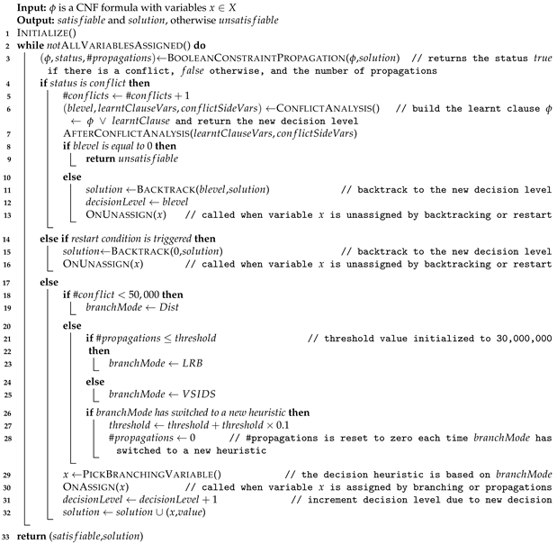
Algorithm 2: Pseudocode for top-level implementation of LSTech.
Algorithms 15 00302 i002

4. The Proposed CDCL SAT Solvers

A description of the proposed CDCL SAT solvers that exploit backbones and backdoors is presented in this section. To begin with, for the purpose of guiding the CDCL SAT solver to branch on backcbones/backdoors, two low-overhead heuristics are proposed for computing backbones and backdoors. They are described in the following subsection.

4.1. Backbone and Backdoor Computational Heuristics

This section details the proposed heuristics for computing the backbone and backdoor sets: backbone low-overhead (BBLO) heuristic and backdoor low-overhead (BDLO) heuristic. Both heuristics are designed based on relevant features of the backbone and backdoor while having low computational overhead. As described below, this trade-off between accuracy and computational time is motivated by the work of [47]. It should be noted that these heuristics are not intended to be standalone heuristics for computing the backbones and backdoors. Rather, they are incorporated within the CDCL SAT solver, in particular the branching heuristic, to encourage the solver to branch on these variables.

4.1.1. The BBLO Heuristic

The BBLO heuristic was inspired by the low-overhead computation of backbones in [47]. Menai and Batouche [47] proposed a backbone-based co-evolutionary algorithm for the partial maximum satisfiability problem guided by the estimated backbone literals of the problem. That is, literals that are set to the same value on each run will be considered backbones; otherwise, they will not. BBLO adopts a similar concept except that local search runs are the search tree trails and non-backbone literals are identified in each run (A trail is the partial assignment that represents the current path in the search tree produced by a CDCL SAT solver.). This process is repeated for each restart.
The BBLO heuristic is presented in Algorithm 3. It is called during every restart procedure in Algorithms 1 and 2. At the first call of the Algorithm 3, all variables in l i s t are marked as undefined. Upon completing a trail, the initial value of the l i s t is its final value of the previous trail. For each assigned variable (line 3), the heuristic determines if it is not a backbone literal whenever a variable has a different assignment than the previous trail (lines 7 and 8). At the end, all assigned variables in L i s t are moved as literals to the backbone set.    
Algorithm 3: A backbone-based low-overhead computational heuristic (BBLO).
Algorithms 15 00302 i003

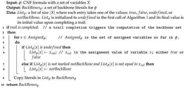
4.1.2. The BDLO Heuristic

The BDLO heuristic is inspired by the findings in [20,21] as well as our findings in Appendix A that show experimentally the near-zero overlap between backbone and LSR backdoor variables on all benchmark categories. Consequently, the BDLO heuristic computes the backdoor variables from the backbones in Algorithm 3. As computed in Algorithm 4, backdoor variables are those that are not backbones (line 9).
Algorithm 4: A backdoor-based low-overhead computational heuristic (BDLO).
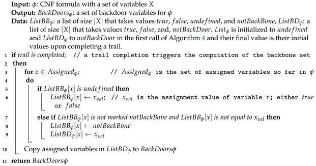
Algorithms 15 00302 i004

4.2. VSIDS Variants

We chose to exploit backbone and backdoor variables by extending the VSIDS heuristic (A detailed description of the VSIDS heuristic is provided in Appendix C.2, along with a justification for choosing the branching heuristic to improve the solver is given in Appendix B.2). The following is a summary of VSIDS’s policy implemented in MapleLCMDistChronoBT-DL-v3 and LSTech:
  • Initialization: Each variable has a floating point number, called activity, which is initialized to 0.
  • Additive bump: Following a conflict analysis phase, the activities of all variables that led to a conflict are additively bumped (increased), typically by 1, if their decision levels are greater than the backtrack level; otherwise, they are bumped by 0.5.
  • Decision: The (unassigned) variable with the highest activity is chosen at each decision.
  • Multiplicative decay: All variables are periodically decremented by multiplying their activities by a constant 0 < D e c a y < 1 called the multiplicative decay factor.
To exploit backbone and backdoor variables, the VSIDS heuristic was extended, specifically, the additive bump policy. We considered the following cases: when to bump, which variables to bump, and with what value to bump. Accordingly, six variants of the VSIDS heuristic were derived: VSIDS_BBsize_restart, VSIDS_BBsize_BBfreq_restart, VSIDS_BBsize_BBfreq_backtrack, VSIDS_BBsize_BBfreq_conflict, VSIDS_BBsize_BBfreq_ restart_conflict, and VSIDS_BDsize_restart. Algorithms 5–10 are variants of the VSIDS, and throughout, we highlight only the added policies to the VSIDS implemented in Maple-based series SAT solvers (see Appendix C.2). For all algorithms, all variables’ activities are initialized to zero. In addition, the backbones and backdoors are computed on every restart by calling BBLO or BDLO. The policy of each variant is detailed below:
1.
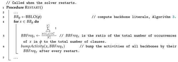
VSIDS_BBsize_restart (Algorithm 5): Following a restart, the activities of the backbone literals computed in Algorithm 3 are additively bumped, typically by 1 (lines 4–5).
Algorithm 5: VSIDS_BBsize_restart a variant of the VSIDS decision heuristic.
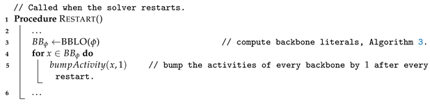
Algorithms 15 00302 i005
2.
VSIDS_BBsize_BBfreq_restart (Algorithm 6): Following a restart, the activities of the backbone literals computed in Algorithm 3 are additively bumped typically by their frequencies (lines 4–6).
Algorithm 6: VSIDS_BBsize_BBFreq_restart a variant of the VSIDS decision heuristic.
Algorithms 15 00302 i006
3.
VSIDS_BBsize_BBfreq_backtrack (Algorithm 7): Following a backtrack, the activities of the backbone literals computed in Algorithm 3 are additively bumped typically by their frequencies (lines 3–4).
Algorithm 7: VSIDS_BBsize_BBFreq_backtrack a variant of the VSIDS decision heuristic.
Algorithms 15 00302 i007
4.
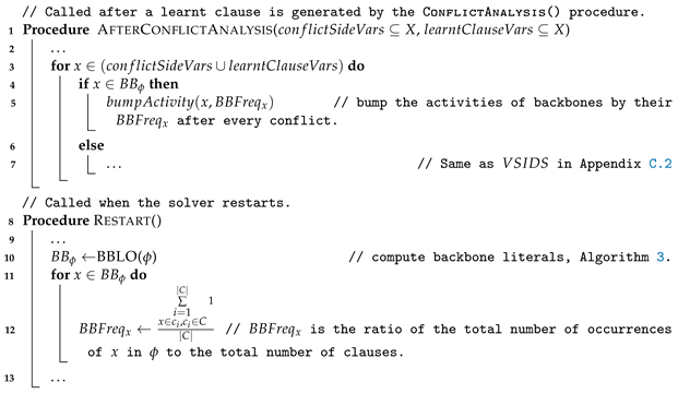
VSIDS_BBsize_BBfreq_conflict (Algorithm 8): Following a conflict, the activities of the backbone literals computed in Algorithm 3 that led to the learnt clause (including those in the learnt clause) are additively bumped typically by their frequencies (lines 3–6).
Algorithm 8: VSIDS_BBsize_BBfreq_conflict a variant of the VSIDS decision heuristic.
Algorithms 15 00302 i008
5.
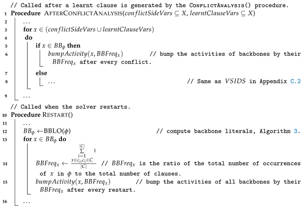
VSIDS_BBsize_BBfreq_restart_conflict (Algorithm 9): In combination of variant 2 and 4.
Algorithm 9: VSIDS_BBsize_BBfreq_restart_conflict a variant of the VSIDS decision heuristic.
Algorithms 15 00302 i009
6.
VSIDS_BDsize_restart (Algorithm 10): Following a restart, the activities of the backdoor variables computed in Algorithm 4 are additively bumped typically by 1 (lines 4–5).
Algorithm 10: VSIDS_BDsize_restart a variant of the VSIDS decision heuristic.
Algorithms 15 00302 i010

4.3. The CDCL SAT Solvers

To demonstrate that the six proposed VSIDS decision heuristics (Algorithms 5–10) contribute to the state of the art, we implemented each of them on top of two base CDCL SAT solvers, MapleLCMDistChronoBT-DL-v3 and LSTech. In doing so, three different versions of the six extended CDCL SAT solvers were developed. In version 1, during restarts/conflicts/backtracks, bumping occurs only in the VSIDS phase. In version 2, bumping during conflicts is only for the VSIDS phase. But, for restarts/backtracks the bumping occurs in both VSIDS and LRB phases (As the bump in VSIDS_BBsize_BBfreq_conflict occurs only during conflicts, it is the same for versions 1 and 2.). Version 3 is the same as version 1, except that in computing the bump with the backbone frequency, the polarity of variables is taken into account (Version 3 is not applicable to the variants VSIDS_BBsize_restart and VSIDS_BDsize_restart.). For convenience, we name each solver by starting with the base solver name, which is followed by the VSIDS variant, and then the version number, e.g., MapleLCMDistChronoBT-DL-v3_VSIDS_BDsize_restart_version1.

5. Performance Evaluation

5.1. Benchmarks and Experimental Setup

Experimental evaluation was performed on industrial benchmark instances drawn from 2002–2021 SAT benchmark instances. On the basis of Table 2, we can see that there are 32 industrial families out of which 12 are satisfiable, 5 are not, and 15 are both. For the purpose of reducing bias, each family contains the same number of satisfiable or/and unsatisfiable instances, seven, and almost the same values of backbone-related measures: backbone size, frequency, and coverage.
The CDCL SAT solvers were evaluated on Shaheen II [48], which is a supercomputer at King Abdullah University of Science and Technology (KAUST). Each node of the cluster is equipped with 128 GB of DDR4 memory and a dual CPU based on 16-core Intel Haswell processors running at 2.3 GHz. In accordance with the literature, the time limit for solving each instance was set at 3600 s. A comparison is presented here between the extended proposed CDCL SAT solvers and their counterpart bases as well as three state-of-the-art winning solvers: RelaxedLCMDCBDL_newTech [15], Kissat_GB [38], and Kissat_MAB [39]. The primary metric is the number of solved instances along with the PAR-2 score. The PAR-2 score is the sum of runtimes for all solved instances and twice the timeout for each unsolved instance, so that a lower score is better.

5.2. Results

The performance results of the six proposed VSIDS extensions implemented in 15 variants of MapleLCMDistChronoBT-DL-v3 and LSTech are presented in Table 3. Each entry represents the number of solved instances. Bold values indicate that the variant performed better than the base solver. MapleLCMDistChronoBT-DL-v3 and LSTech solved 302 and 308, respectively, out of 329 industrial instances. The best performing variant for each base solver is MapleLCMDistChronoBT-DL-v3_VSIDS_BBsize_BBfreq_restart_version2 (Maple_VBBsfr_v2) and LSTech_VSIDS_BBsize_BBfreq_restart_conflicts_version1 (LSTech _VBBsfrc_v1). Maple_VBBsfr_v2 solved 307 instances, which was five more than the base solver. With LSTech_VBBsfrc_v1, four more instances were solved than with the base solver. For the solvers based on VSIDS_BDsize_restart, the only variant that improved is LSTech_VSIDS_ BDsize_restart_version1. Furthermore, note that the solver variants based on backtracks (row number 3) did not perform well.
The scatter plots shown in Figure 2a,b detail performance comparisons of Maple_ VBBsfr_v2 and LSTech_VBBsfrc_v1 to their base solvers. Each improved variant solved more instances and achieved a lower PAR-2 score than its base counterpart.
Table 4 and Figure 3 report runtime results of Maple_VBBsfr_v2 and LSTech_VBBsfrc_v1 compared to state-of-the-art CDCL SAT solvers on the whole benchmark instances in Table 2. It is observed that LSTech_VBBsfrc_v1 scored 312, which is one instance more than the number of instances solved by Kissat_MAB, the winner of the 2021 SAT competition. According to Table 4 and Figure 4a,b, Maple_VBBsfr_v2 showed improvements on both satisfiable and unsatisfiable benchmarks, while LSTech_VBBsfrc_v1 showed improvements on satisfiable benchmarks.

6. Discussion

Backbones and backdoors have been introduced for over two decades, but the current state of the art of CDCL SAT solvers [17,49] shows limited evidence of their use to improve CDCL SAT solvers. Among the few is Dequen and Dubois’ work [24]. The backbone-guided decision heuristic they proposed was heavily dependent on unit propagation, which consequently added a significant overhead to the solver performance. It should be noted that early in our work, we have implemented the backbone guided decision heuristic [24] on top of MapleLCMDistChronoBT-DL-v3 to compute backbones; however, the solver performed poorly and never beat the base solver. In addition, it was demonstrated in [19,50] that it is difficult to build a solver that detects backdoors due to the difficulty of computing them. In this regard, we have proposed the BBLO and BDLO heuristics for computing backbones and backdoors. As far as backdoors, they are calculated under the assumption of no overlap between backbones and backdoors, which is only an experimental observation.
According to the performance evaluation in Section 5, both variants Maple_VBBsfr_v2 and LSTech_VBBsfrc_v1 have outperformed the base solvers on solving satisfiable benchmarks, that is, instances with backbones. Therefore, improvements in VSIDS have led to improved performance for both variants in solving more satisfiable instances. It is therefore evident that VSIDS is not only superior at solving unsatisfiable instances [51] but could even be improved to solve satisfiable instances as well.
Further observations include the improved performance of Maple_VBBsfr_v2 with both satisfiable and unsatisfiable benchmarks, while LSTech_VBBsfrc_v1 only improved with satisfiable benchmarks. Evidence suggests that the BBLO heuristic could assist the CCAr solver in finding an earlier solution by identifying promising partial assignments.

7. Conclusion and Future Work

In this study, we performed a set of modifications to the VSIDS decision heuristic to exploit backbones and backdoors. To guide the CDCL SAT solver to branch on backbone/backdoor variables, we proposed low-overhead heuristics to compute them. We implemented 15 variants on top of two popular state-of-the-art award-winning CDCL solvers, MapleLCMDistChronoBT-DL-v3 and LSTech. The variants were evaluated on 32 industrial families from 2002 to 2021 SAT competitions. Results showed that bumping the backbone and backdoor variables during the branching heuristic improved both solvers’ performance. In particular, the variant of LSTech that augmented the VSIDS decision heuristic to exploit the backbone size and frequency and bumped during restarts and conflicts solved more industrial instances compared to the best state-of-the-art CDCL solvers. In the future, we would like to assess the accuracy of the proposed backbone and backdoor heuristics and to investigate the possibility of any improvements. A further research goal would be to modify other decision heuristics, such as LRB and CHB. Moreover, we would like to conduct a larger study to include broader bases of CDCL SAT solvers and benchmarks.

Author Contributions

Conceptualization, T.A.-Y. and M.E.B.A.M.; methodology, T.A.-Y. and M.E.B.A.M.; software, T.A.-Y.; validation, T.A.-Y. and M.E.B.A.M.; formal analysis, T.A.-Y. and M.E.B.A.M.; investigation, T.A.-Y. and M.E.B.A.M.; resources, T.A.-Y. and M.E.B.A.M.; data curation, T.A.-Y.; writing—original draft preparation, T.A.-Y.; writing—review and editing, T.A.-Y. and M.E.B.A.M.; supervision, M.E.B.A.M. and H.M. All authors have read and agreed to the published version of the manuscript.

Funding

The authors would like to thank the Deanship of Scientific Research (DSR) in King Saud University for funding and supporting this research through the initiative of DSR Graduate Students Research Support (GSR).

Institutional Review Board Statement

Not applicable.

Informed Consent Statement

Not applicable.

Data Availability Statement

The datasets generated during the current study are not publicly available but are available from the corresponding author on reasonable request.

Acknowledgments

We are grateful to the KAUST Supercomputing Laboratory for the use of Shaheen II (https://www.hpc.kaust.edu.sa (accessed on 15 January 2020)). We thank them for providing the computational resources and professional support for carrying out this work.

Conflicts of Interest

The authors declare no conflict of interest.

Appendix A. The Evidence of Boolean Structural Measures for SAT

Boolean structure measures well known in the literature are: phase transition, backbone size, backdoor size, and backbone/backdoor variable overlap size [25]. In view of the fact that the phase transition is only located for random and industrial-like instances, we focus on characterizing SAT instances based on backbones and backdoors. Interest in backbone and backdoor size was originally motivated to relate them to problem hardness and the performance of the SAT solver [20]. Backbones have been used to guide the variable decision heuristics for SAT solvers [24]. Insight into the heavy-tailed phenomena observed in backtrack heuristics comes from considering backdoor variables. Intuitively, backtrack heuristics appear to be lucky on certain runs due to small (near-zero) backdoor sizes. Consequently, backdoor variables are identified early and set correctly [31,49,52]. Boolean structural measures examined are the backbone size, backdoor size, and backbone/backdoor variable overlap size. We also introduced three new related measures: backbone frequency, backbone coverage, and backdoor coverage. All measures are defined in Section 2 except for backbone coverage and backdoor coverage, which are defined below:
Definition A1
(Backbone coverage). Backbone coverage is the percentage proportion of clauses that contains backbone literals in a CNF formula (after CNF formula simplification), denoted B B c v g ϕ . Backbone coverage is expressed as follows:
B B c v g ϕ = i = 1 , x b B B ϕ x b C i s . t . C i C | C | 1 | C | × 100
Definition A2
(Backdoor coverage). Backdoor coverage is the percentage number of clauses that contain backdoor variables in a CNF formula (after CNF formula simplification), denoted B D c v g ϕ . This is formulated as follows:
B D c v g ϕ = i = 1 , x B D ϕ x C i s . t . C i C | C | 1 | C | × 100

Appendix A.1. Backbone and Backdoor Computation

To demonstrate the presence of backbones and backdoors for SAT instances, we calculated these measures across the entire benchmark sets. Backbones were computed exactly by the tool in [42]. This tool is based on repeated calls to MiniSat. Based on the backbone sets, the frequencies and coverages of the backbone sets were calculated as shown in Equations (3) and (A1).
LSR-backdoors were computed using a tool developed by [19] called LaSeR. Due to the difficulty of exactly computing the LSR-backdoors, the tool was configured to compute an upper bound on the size of the minimal LSR-backdoor. The tool is built on top of the MapleSAT solver [14]. After the backdoor sets were computed, the backdoor coverages were calculated, as shown in Equation (A2). Finally, the backbone/backdoor overlap was computed based on Equations (6) and (7).

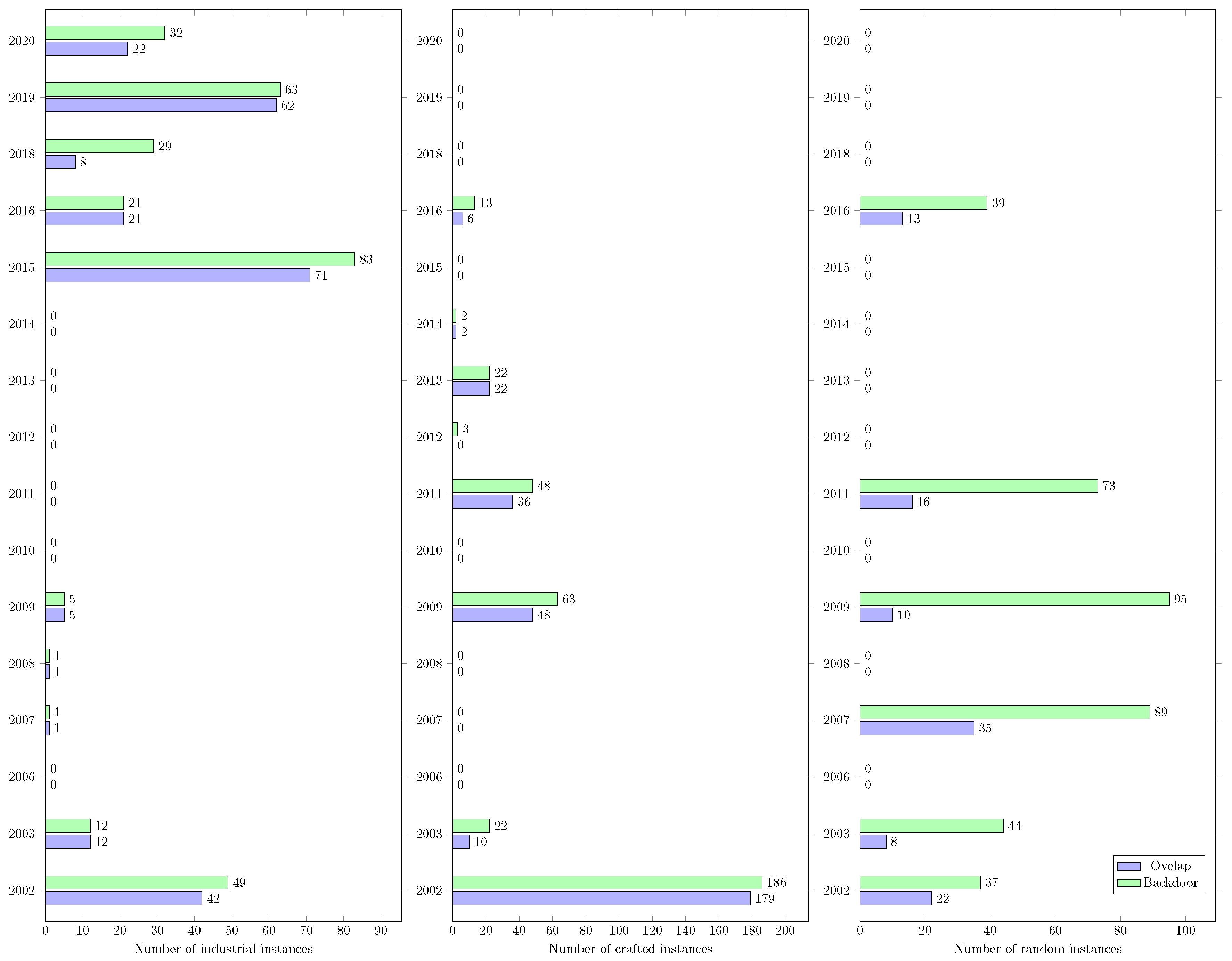
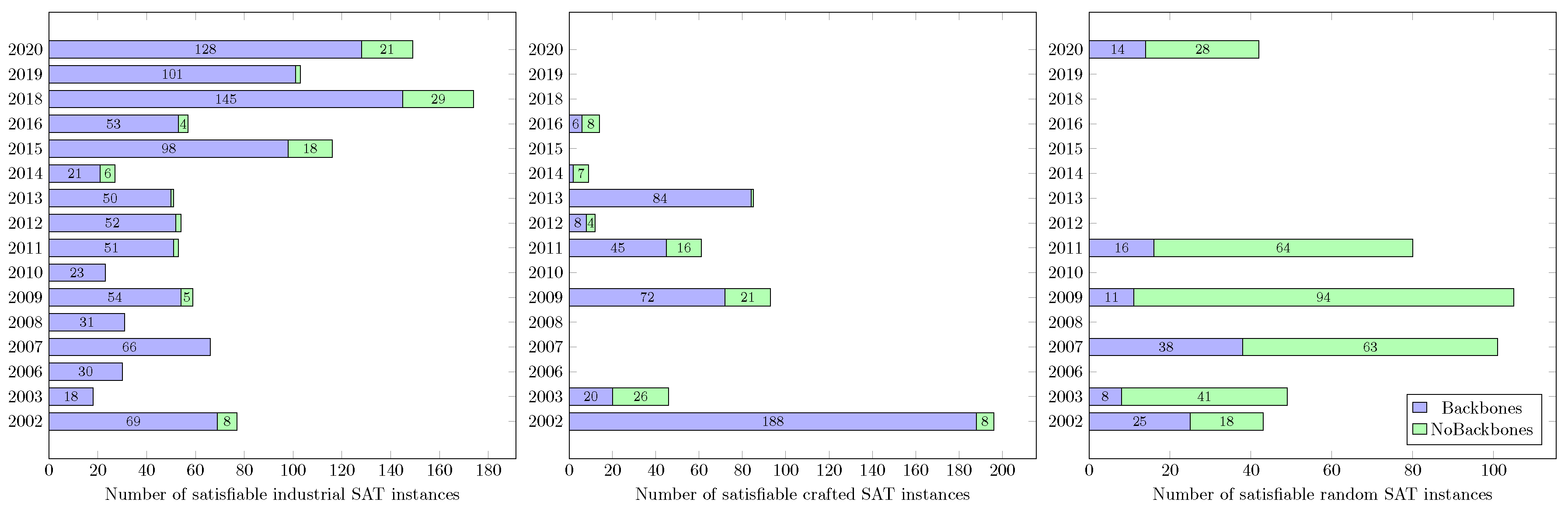
Appendix A.2. Benchmarks and Experimental Setup

Experiments were conducted on Shaheen II [48]. A timeout period of 72 h was set to compute all backbone-related measures (backbone size, backbone frequency, and backbone coverage) and similarly for backdoor-related measures (backdoor size, backdoor coverage, and backbone/backdoor variable overlap size) for each of the 7779 instances (see Table A1) (We were unable to locate benchmarks for 2004, 2005, or 2017).
Table A1. Number of instances included in experiments drawn from 2002–2020 SAT benchmarks. The symbol × means that no instances were submitted under the corresponding category.
YearIndustrialCraftedRandom
200220954197
200369259138
200670××
200716116406
200862××
2009165159570
2010100××
2011150150613
201220853600
2013150201430
201458121225
2015176××
2016182200240
2018400××
2019200××
2020400××

Appendix A.3. Experimental Results

We computed the backbones for all satisfiable instances presented in Table A1. In Figure A1, we report the number of satisfiable instances in each benchmark category with and without backbones. In contrast to random instances, most satisfiable industrial and crafted instances preserve the backbone structure. It is due to the fact that the backbone sizes for most random instances are controlled by being set to zero prior to generation.
Figure A1. Number of instances with (w∖o) backbones on 2002–2020 SAT benchmarks.
Algorithms 15 00302 g0a1
Structural measures related to backdoors are computed on all satisfiable and unsatisfiable SAT benchmark instances (see Table A1). Figure A2 displays the number of satisfiable and unsatisfiable instances with backdoors. One point to note is that the reported instances for backdoors are lower than those for backbones. This is due to the hardness of computing LSR backdoors [53]. The number of satisfiable instances with backbone/backdoor variable overlap is shown in Figure A3.
All Boolean measures are computed, along with their means and standard deviations. A summary of the results is presented in Table A2. Empirical results indicate that most random benchmarks have no backbones, whereas on average, industrial and crafted benchmark instances have small backbone sizes. The frequency of backbones is low for all benchmark categories. As for the backbone coverage, industrial and crafted benchmarks have higher coverages, on average, than random ones. In both crafted and random benchmark instances, the backdoor size and coverage are greater than those in the industrial category. Additionally, across all SAT benchmarks, there tends to be little overlap between backbone and backdoor variables.
Figure A2. Number of satisfiable/unsatisfiable instances with backdoors on 2002–2020 SAT benchmark instances.
Algorithms 15 00302 g0a2
Figure A3. Number of instances with backbone/backdoor variable overlap on 2002–2020 SAT benchmark instances.
Algorithms 15 00302 g0a3
Table A2. Mean (standard deviation) of the normalized values of Boolean structural measures on 2002–2020 SAT benchmark instances.
IndustrialCraftedRandom
Backbone size0.13 (0.2)0.26 (0.39)0.06 (0.23)
Backbone frequency0.05% (0.18)0.34% (1.14)1.09% (3.63)
Backbone coverage15.22% (23.92)28.49% (40.33)6.71% (23.74)
Backdoor size0.67 (0.31)0.88 (0.2)0.98 (0.08)
Backdoor coverage83.41% (25.1)95.18% (12.73)99.61% (3.49)
Backbone/backdoor variable overlap0.08 (0.1)0.29 (0.36)0.22 (0.4)

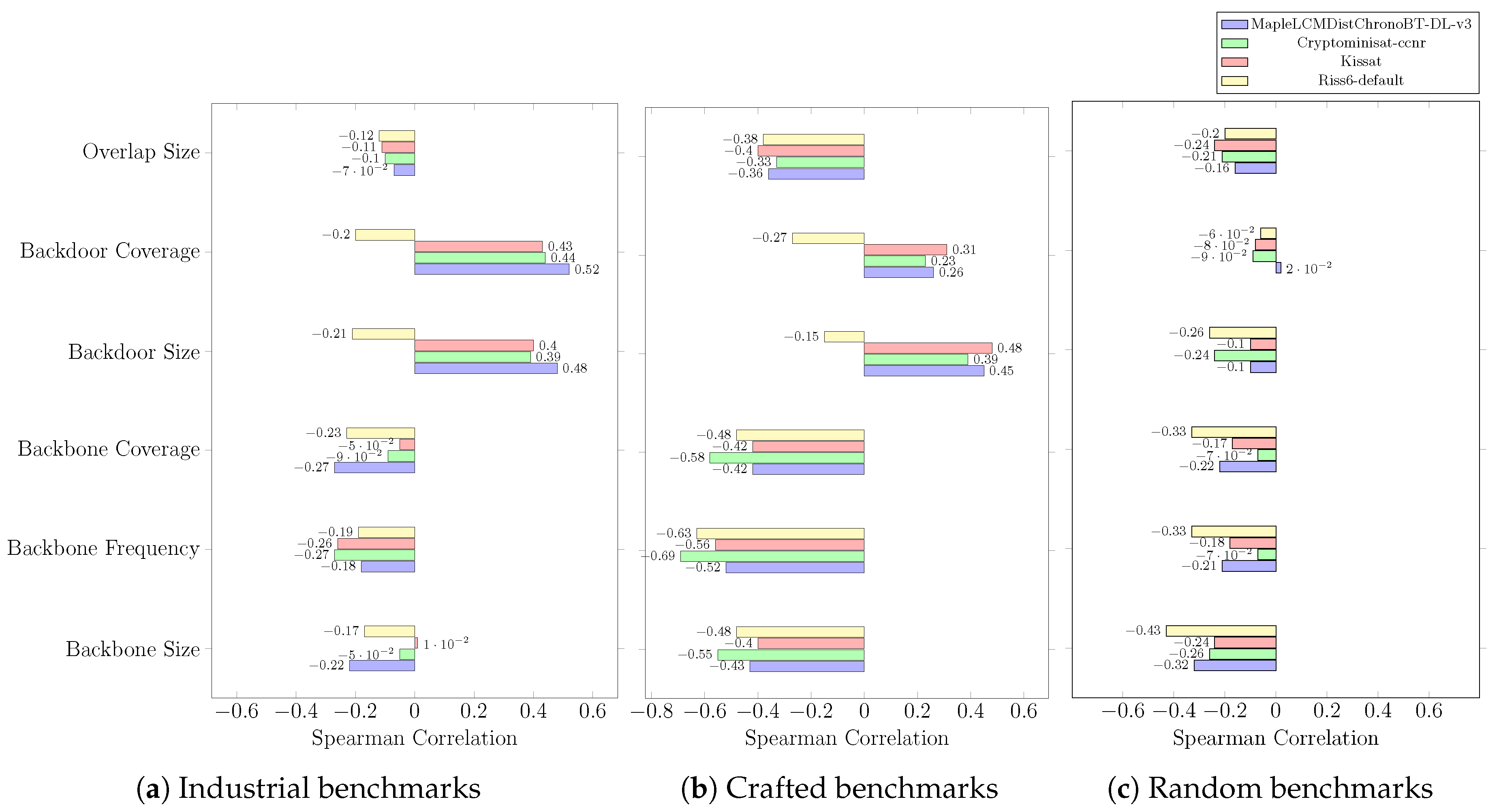
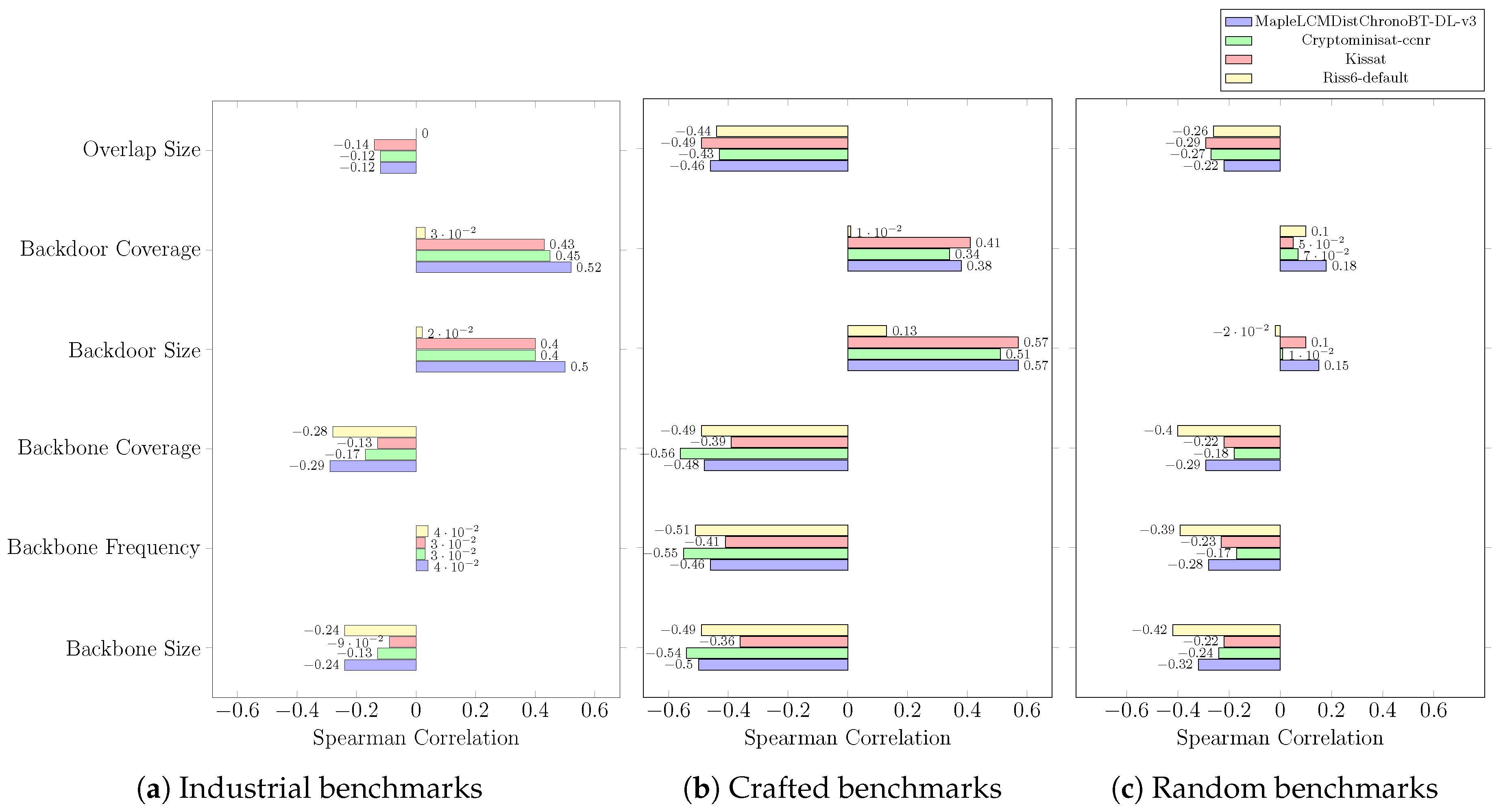
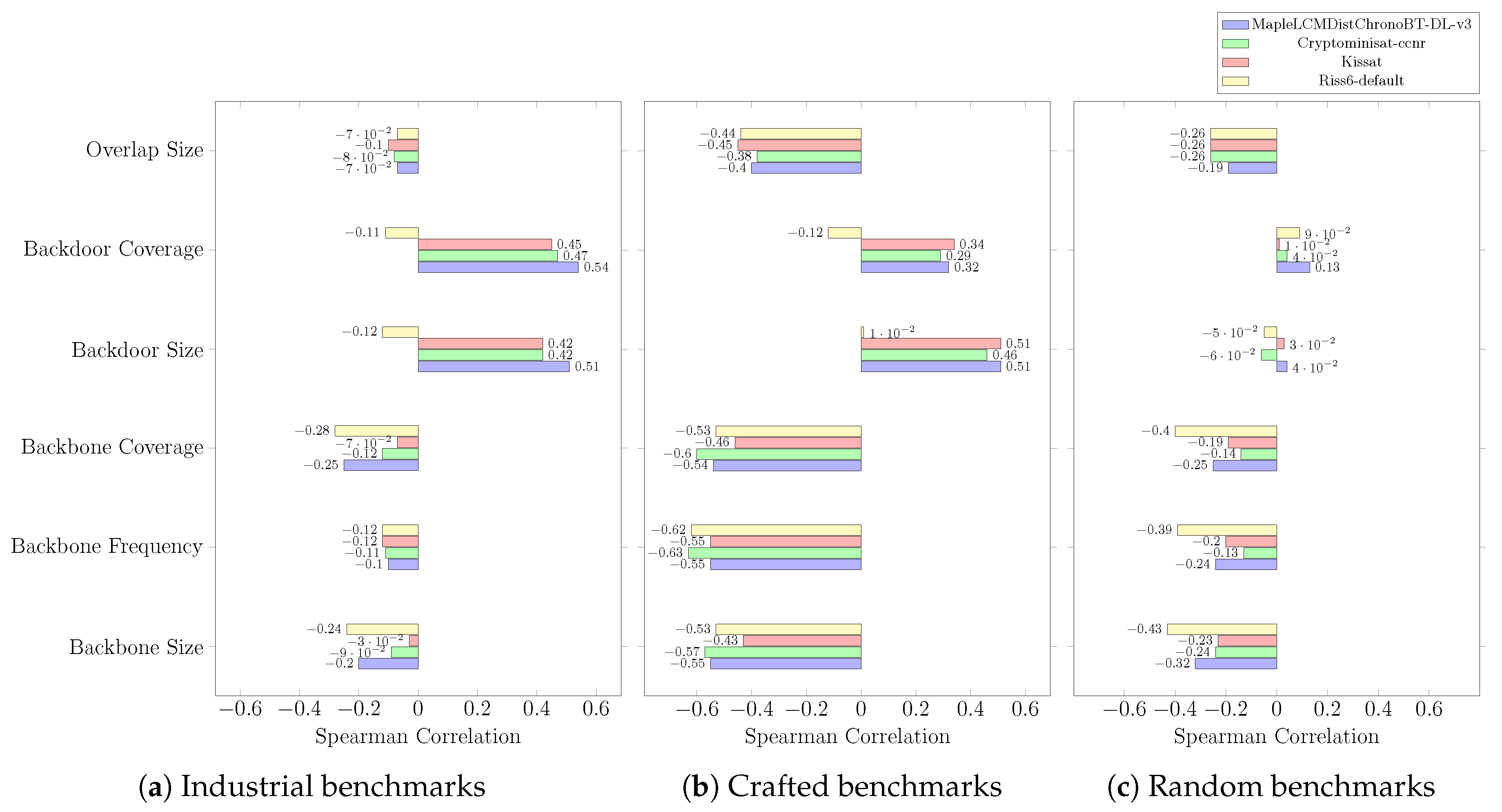
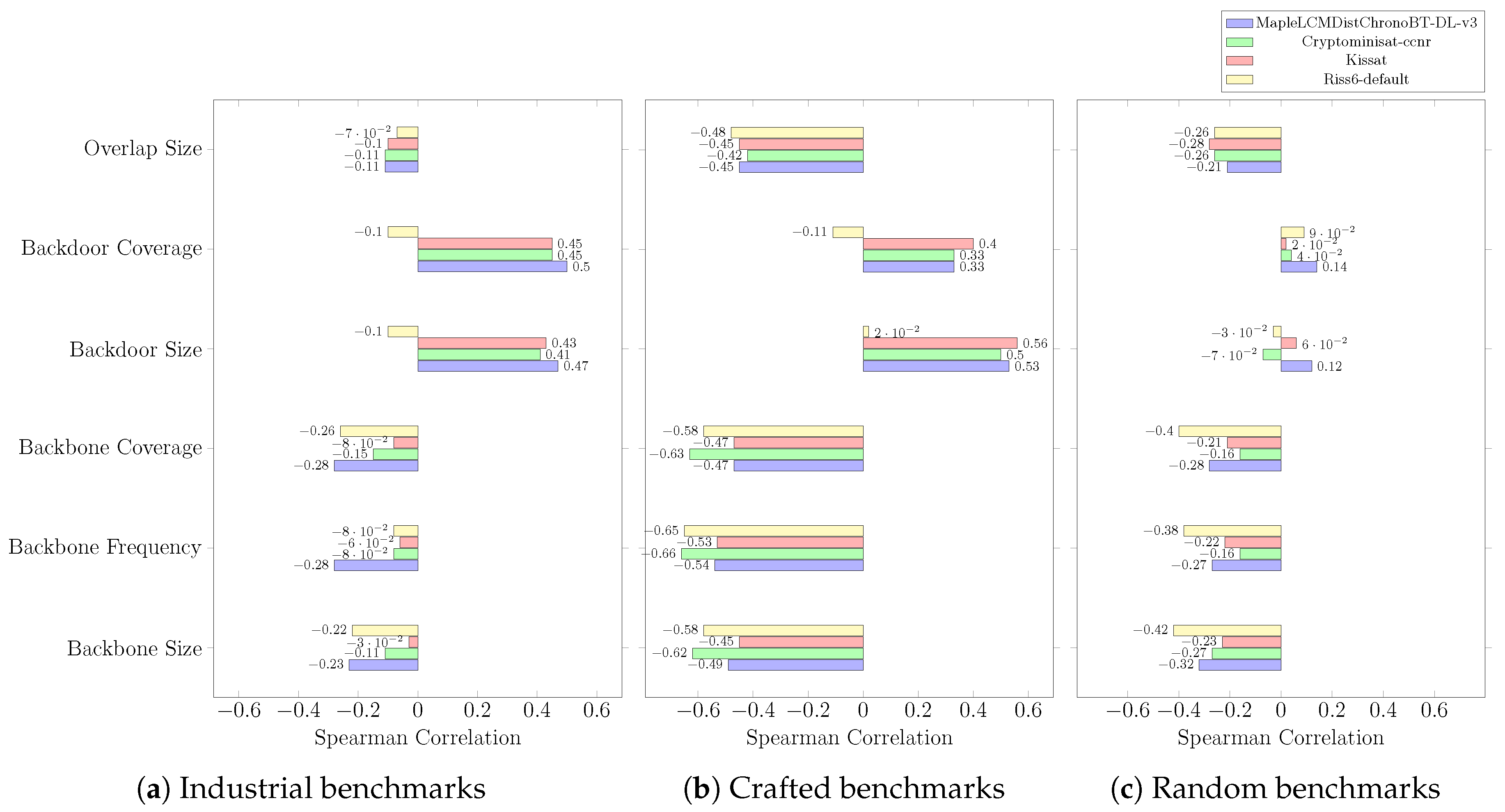
Appendix B. Correlation and Exploitation Analysis

Appendix B.1. Correlation Analysis

Correlation analysis was carried out to quantify the strength and direction of the relation between the Boolean structural measures and the CDCL metrics. In particular, we computed the Spearman correlation coefficient to measure the nonlinear dependency between two random variables: the Boolean structural measures and CDCL metrics. Four CDCL solver metrics were evaluated: runtime, number of decisions, number of propagations, and number of conflicts. These metrics are derived from the essential blocks that make up any CDCL solver. The CDCL-based solvers that were examined are MapleLCMDistChronoBT-DL-v3, CryptoMiniSat-ccnr, Kissat, and Riss6-default. In choosing these solvers, we primarily considered their superior performance in SAT competitions and the unique differences in techniques incorporated and implementation.
Experiments were conducted on Shaheen II [48] and carried out on SAT instances presented in Table A1. A timeout period of 72 h was set to compute the four metrics runtime, number of decisions, number of propagation, and number of conflicts required by the solvers: MapleLCMDistChronoBT-DL-v3, CryptoMiniSat-ccnr, Kissat, and Riss6-default for each of the 7779 SAT instances. As for the backbone and backdoor measures, they were computed as specified in Appendix A.
Results are depicted in Figure A4, Figure A5, Figure A6 and Figure A7. The results show that CDCL metrics are inversely proportional to backbone-related measures and backbone/backdoor overlap size, but they are proportional to backdoor-related measures across all industrial, crafted, and random benchmark instances. In addition, correlation results are apparent for structured instances. Finally, correlation results are more evident for MapleLCMDistChronoBT-DL-v3 on industrial benchmarks. Based on this, MapleLCMDistChronoBT-DL-v3 was selected as the base solver in our research, along with LSTech, which is an improvement of MapleLCMDistChronoBT-DL-v3 and a medal winner of the 2021 SAT competition.
Figure A4. Spearman correlation results between Boolean structural measures and the CPU time on 2002–2020 SAT benchmark instances.
Algorithms 15 00302 g0a4
Figure A5. Spearman correlation results between Boolean structural measures and the number of decisions on 2002–2020 SAT benchmark instances.
Algorithms 15 00302 g0a5
Figure A6. Spearman correlation results between Boolean structural measures and the number of propagations on 2002–2020 SAT benchmark instances.
Algorithms 15 00302 g0a6
Figure A7. Spearman correlation results between Boolean structural measures and the number of conflicts on 2002–2020 SAT benchmark instances.
Algorithms 15 00302 g0a7

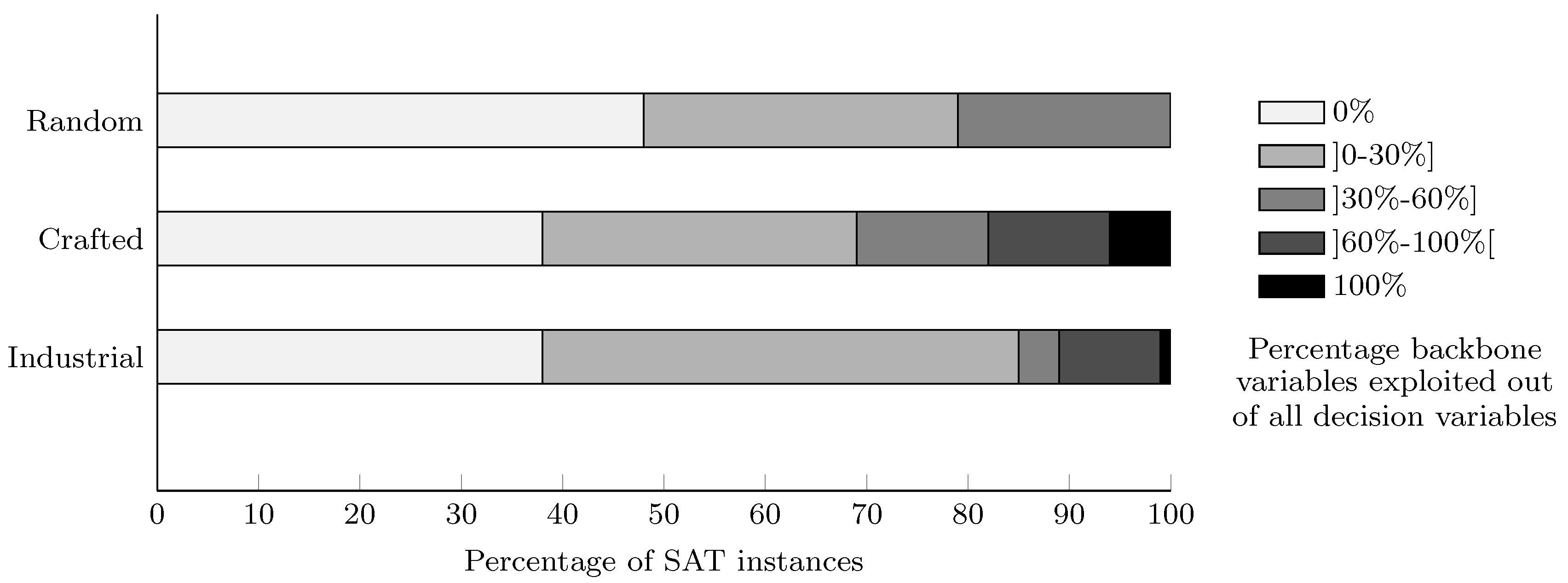
Appendix B.2. Exploitation Analysis

Following the correlation results described in Appendix B.1, MapleLCMDistChronoBT-DL-v3 was used to carry out the rest of the analysis and experiments. As a way of examining whether MapleLCMDistChronoBT-DL-v3 exploits Boolean structural measures, we determined the percentage number of backbone variables decided for the solver in the first 1000 iterations. The experiments were limited to only backbone variables, not backdoors, since backbones are unique in SAT instances while backdoors are not. Therefore, determining whether backdoor variables are exploited is challenging.
Experiments were conducted, as before, on Shaheen II [48] and carried out on satisfiable SAT instances with backbones computed from 2002–2020 SAT benchmark instances (see Figure A1). The decision variables for the first 1000 decisions ran by MapleLCMDistChronoBT-DL-v3 were collected.
The percentage of exploited backbones performed by MapleLCMDistChronoBT-DL-v3 for the first 1000 decisions on all 2002–2020 benchmark instances is displayed in Figure A8. Generally, it seems that the percentage of exploited backbones varies more on industrial and crafted benchmark instances than on random ones. In addition, for structured instances, there appears to be a percentage number of instances where all backbone variables are exploited.
Furthermore, we analyzed the percentage of exploited backbones for SAT instances that have been solved in less than 1000 decisions for all benchmark categories. Each row in Table A3, Table A4 and Table A5 (In the case of crafted instances, we grouped three instances per row for convenience.) identifies an instance, highlighting the number of decisions required to solve it (first column) and the percentage backbone variables exploited (second column). For instances that can be solved in less than 1000 decisions, it is obvious that structured instances exploit most of the backbone variables. On the other hand, less than 50% of backbone variables are exploited for random benchmark instances.
Figure A8. Percentage number of exploited backbones by MapleLCMDistChronoBT-DL-v3 for the first 1000 decisions on all 2002–2020 benchmark instances.
Algorithms 15 00302 g0a8
Table A3. Reported industrial instances from experiment in Figure A8 that are solved in fewer than 1000 decisions.
Number of
Decisions
Percentage of Exploited Backbones
in All Decision Variables
37054.05%
1566.67%
18070.00%
37291.67%
33595.52%
17499.43%
3100.00%
36100.00%
49100.00%
55100.00%
57100.00%
57100.00%
60100.00%
152100.00%
Table A4. Reported crafted instances from experiment in Figure A8 that are solved in fewer than 1000 decisions.
Number of
Decisions
Percentage of Exploited
Backbones in All
Decision Variables
Number of
Decisions
Percentage of Exploited
Backbones in All
Decision Variables
Number of
Decisions
Percentage of Exploited
Backbones in All
Decision Variables
1855.56%4486.36%116100.00%
1957.89%36992.68%144100.00%
94058.62%18498.37%188100.00%
56358.79%25898.84%208100.00%
35261.08%21599.07%229100.00%
44361.63%21799.08%239100.00%
71662.15%22499.11%276100.00%
53463.11%17399.42%281100.00%
78963.88%16100.00%298100.00%
49065.51%26100.00%300100.00%
16067.50%30100.00%323100.00%
6170.49%88100.00%346100.00%
2272.73%99100.00%351100.00%
2281.82%106100.00%401100.00%
3381.82%109100.00%435100.00%
Table A5. Reported random instances from experiment in Figure A8 that are solved in fewer than 1000 decisions.
Number of
Decisions
Percentage of Exploited Backbones
in All Decision Variables
6947.83%
16947.93%
67848.82%
35249.72%
66749.93%
19150.79%
39151.15%
15651.28%
59453.20%
65653.20%
31253.53%
40454.21%

Appendix C. The CDCL Framework and Popular Variable Decision Heuristics

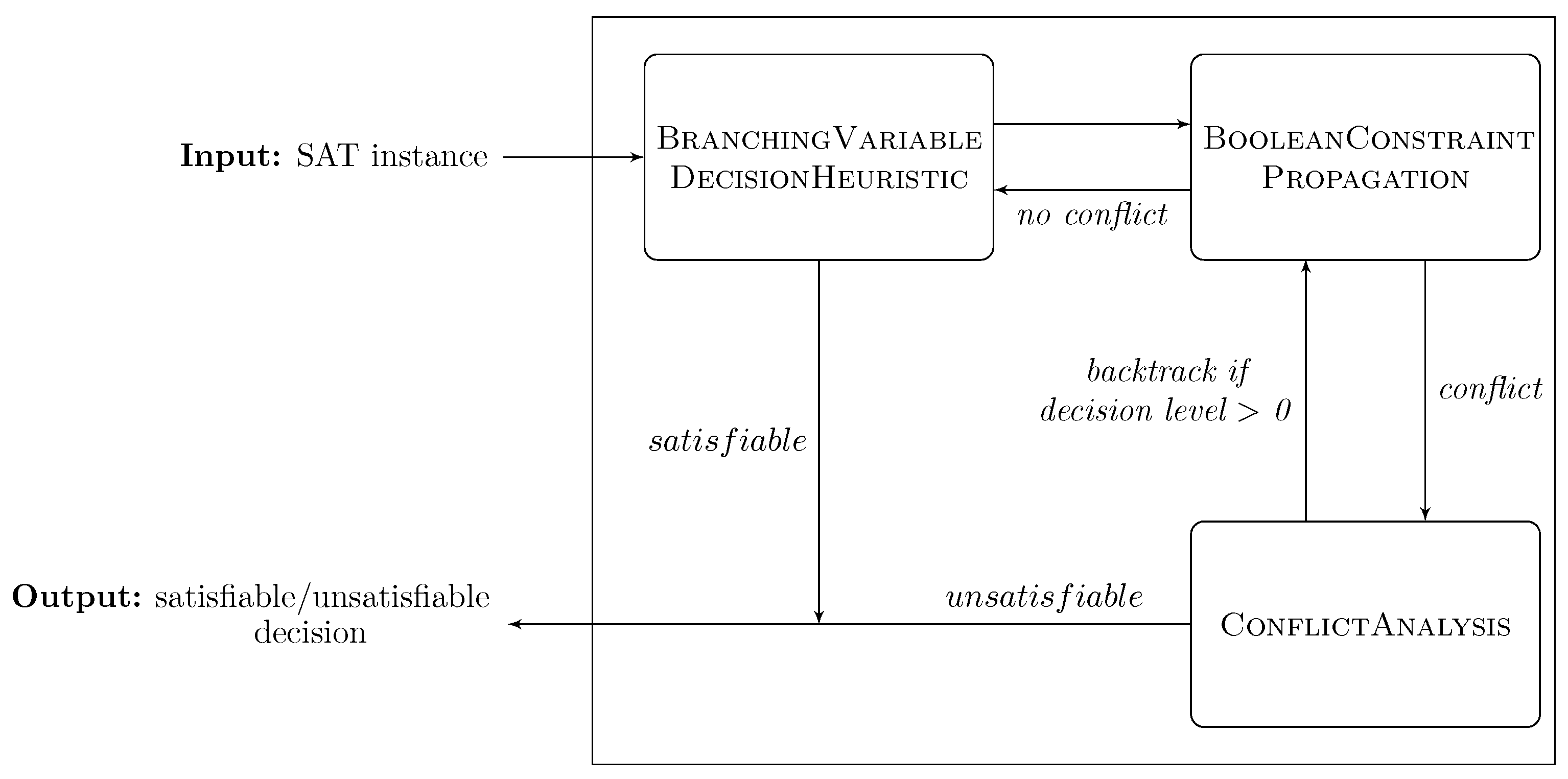
Appendix C.1. The CDCL Framework

The CDCL framework is depicted in Algorithm A1. After constraint propagation detects a conflict (lines 3–4), CDCL learns at least one reason for that conflict in the form of a new clause (lines 5 and 6), called learnt clause, which is added to the CNF formula. In this case, the CDCL SAT solver directly backtracks to an earlier level (lines 9–12). The instance is declared unsatisfiable if the backtracked level is zero. In the absence of a conflict, a branching variable is picked and the level of that variable is updated accordingly (lines 18–21). Once all variables are assigned, the formula is satisfied (line 2). In the event that the restart condition is triggered, the SAT solver will restart (lines 13–16).
Algorithm A1: CDCL framework.
Algorithms 15 00302 i011

Appendix C.2. The VSIDS Heuristic

VSIDS refers to a class of branching heuristics commonly used in CDCL SAT solvers that rank all the variables in an SAT instance during the run of the solver. VSIDS is significantly more effective than other well-known heuristics, particularly when solving unsatisfiable SAT instances [51,54,55]. The VSIDS heuristic was originally proposed as part of the Chaff solver [6]. Since then, many variants have been proposed, including VSIDS implemented in MiniSat and the variable move-to-front (VMTF) decision heuristic. In general, VSIDS is characterized by additive bumping, multiplicative decay, and low computation overhead. This work will focus on the VSIDS MiniSat variant implemented in Maple-based series SAT solvers [56].
The policy of VSIDS implemented in Maple-based series SAT solvers [56] is presented in Algorithm A2. All procedures are called as part of the CDCL framework in Algorithm A1. In the initialization procedure (line 1), each variable has a floating point number, called activity, which is initialized to 0 (lines 4–7). Following a conflict analysis phase (line 9), the activities of all variables that led to the learnt clause (including those in the learnt clause) are additively bumped (increased), typically by 1, if their decision levels of variables are greater than the backtrack level, such variables receive more bumps to activity scores (line 14); otherwise, they are bumped by 0.5 (line 16). In addition, all activities of variables are decremented by multiplying them by a constant 0 < D e c a y < 1 called the multiplicative decay factor (lines 18–20). To select a variable, the (unassigned) variable and polarity with the highest activity are chosen at each decision (line 24).
Algorithm A2: VSIDS decision heuristic. All procedures are part of the CDCL framework in Algorithm A1.
Algorithms 15 00302 i012

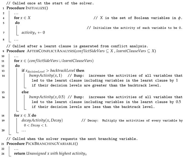
Appendix D. Reported Results on Industrial Families

Table A6. The number of solved instances of industrial families from the 2002–2021 SAT competitions. Each family consists of seven satisfiable instances.
FamilyMapleLCM
DistChrono
BT-DL-v3
Maple_
VBBsfr_v1
LSTechLSTech_
VBBsfrc_v2
Relaxed_
LCMDCBDL_
newTech
Kissat_GBKissat_MAB
aloul_bart7777777
goldberg7777777
grastien_anbulagan_diag7777777
grastien_anbulagan_medium7777777
rintanen5657645
soos5657655
Argumentation7777767
StedmanTriples7777667
MinimalSuperpermutation6777667
biere_dinphil7777777
eichberger7777777
manthey_cvc46576677
corblin7777777
cryptanalysis_zaikin7777777
surynek7777777
stojadinovic7777777
zarpas_Ibm7777777
manthey_stp7777777
HamiltonianCycle7745477
fuhs_aes5466667
MaxsatOptimum7777777
CircuitMultiplie6577666
GiraldezCr7777777
scheduling7777717
PetrinetConcurrency5777737
velve7777777
ehlers4455646
Total175177179183178166183
Table A7. The number of decided unsatisfiable instances of industrial families from the 2002–2021 SAT competitions. Each family consists of seven unsatisfiable instances.
FamilyMapleLCMDistChronoBT-DL-v3Maple_VBBsfr_v1LSTechLSTech_
VBBsfrc_v2
Relaxed_LCMDCBDL_newTechKissat_GBKissat_MAB
rintanen6777766
eichberger7777777
stojadinovic7777777
surynek7777777
GiraldezCr6766666
manthey_cvc44554554
manthey_stp5555555
ehlers6666666
zaikin7777777
goldberg5667676
biere_dinphil7777777
velve7777777
zarpas_Ibm7777777
corblin7777777
AtLeastTwoSolutions7777777
CellularAutomata7777777
strcmpVerification7777777
lamProblem6666666
populationSafety7777776
fuhs_aes5444366
Total127130129129128131128

References

  1. Cook, S.A. The Complexity of Theorem-proving Procedures. In Proceedings of the Third Annual ACM Symposium on Theory of Computing, Shaker Heights, OH, USA, 3–5 May 1971; pp. 151–158. [Google Scholar] [CrossRef]
  2. Lai, K.; Siewiorek, D.P. Functional testing of digital systems. In Proceedings of the 20th Design Automation Conference, DAC ’83, Miami Beach, FL, USA, 27–29 June 1983; pp. 207–213. [Google Scholar]
  3. Clarke, E.M.; Emerson, E.A. Design and synthesis of synchronization skeletons using branching time temporal logic. In Proceedings of the Logics of Programs, Yorktown Heights, NY, USA, 1982; Kozen, D., Ed.; Springer: Berlin/Heidelberg, Germany, 1982; pp. 52–71. [Google Scholar]
  4. D’Silva, V.; Kroening, D.; Weissenbacher, G. A Survey of Automated Techniques for Formal Software Verification. IEEE Trans. Comput. Aided Des. Integr. Circuits Syst. 2008, 27, 1165–1178. [Google Scholar] [CrossRef]
  5. SAT Competitions. 2002. Available online: http://www.satcompetition.org (accessed on 19 November 2019).
  6. Moskewicz, M.W.; Madigan, C.F.; Zhao, Y.; Zhang, L.; Malik, S. Chaff: Engineering an efficient SAT solver. In Proceedings of the 38th Design Automation Conference (IEEE Cat. No.01CH37232), Las Vegas, NV, USA, 22 June 2001; pp. 530–535. [Google Scholar] [CrossRef]
  7. Luby, M.; Sinclair, A.; Zuckerman, D. Optimal speedup of Las Vegas algorithms. Inf. Process. Lett. 1993, 47, 173–180. [Google Scholar] [CrossRef]
  8. Audemard, G.; Simon, L. Predicting Learnt Clauses Quality in Modern SAT Solvers. In Proceedings of the 21st International Jont Conference on Artifical Intelligence, Pasadena, CA, USA, 11–17 July 2009; IJCAI’09. pp. 399–404. [Google Scholar]
  9. Luo, M.; Li, C.M.; Xiao, F.; Manyà, F.; Lü, Z. An Effective Learnt Clause Minimization Approach for CDCL SAT Solvers. In Proceedings of the Twenty-Sixth International Joint Conference on Artificial Intelligence, IJCAI-17, Melbourne, Australia 19–25 August 2017; pp. 703–711. [Google Scholar] [CrossRef]
  10. Xiao, F.; Luo, M.; Li, C.M.; Manyà, F.; Lü, Z. MapleLRB LCM, Maple LCM, Maple LCM Dist, MapleLRB LCMoccRestart and Glucose-3.0+width in SAT Competition 2017. In Proceedings of the SAT Competition 2017: Solver and Benchmark Descriptions, Melbourne, Australia, 28 August–1 September 2017; Volume B-2017-1, pp. 25–26. [Google Scholar]
  11. Nadel, A.; Ryvchin, V. Chronological Backtracking. In Proceedings of the Theory and Applications of Satisfiability Testing—SAT 2018, Oxford, UK, 9–12 July 2018; Beyersdorff, O., Wintersteiger, C.M., Eds.; Springer International Publishing: Cham, Switzerland, 2018; pp. 111–121. [Google Scholar]
  12. Kochemazov, S.; Zaikin, O.; Semenov, A.A.; Kondratiev, V. Speeding Up CDCL Inference with Duplicate Learnt Clauses. In Proceedings of the ECAI 2020—24th European Conference on Artificial Intelligence, Santiago de Compostela, Spain, 29 August–8 September 2020; Giacomo, G.D., Catalá, A., Dilkina, B., Milano, M., Barro, S., Bugarín, A., Lang, J., Eds.; IOS Press: Shepherdsville, KY, USA, 2020; Volume 325, pp. 339–346. [Google Scholar] [CrossRef]
  13. Liang, J.H.; Ganesh, V.; Poupart, P.; Czarnecki, K. Exponential Recency Weighted Average Branching Heuristic for SAT Solvers. In Proceedings of the Thirtieth AAAI Conference on Artificial Intelligence, Phoenix, AZ, USA, 12–17 February 2016; AAAI’16. pp. 3434–3440. [Google Scholar]
  14. Liang, J.H.; Ganesh, V.; Poupart, P.; Czarnecki, K. Learning Rate Based Branching Heuristic for SAT Solvers. In Proceedings of the Theory and Applications of Satisfiability Testing—SAT 2016—19th International Conference, Bordeaux, France, 5–8 July 2016; Creignou, N., Berre, D.L., Eds.; Springer: Berlin/Heidelberg, Germany, 2016; Volume 9710, pp. 123–140. [Google Scholar] [CrossRef]
  15. Zhang, X.; Cai, S. Relaxed Backtracking with Rephasing. In Proceedings of the SAT Competition 2020, Alghero, Italy, 3–10 July 2020; Solver and Benchmark Descriptions. University of Helsinki, Department of Computer Science: Helsinki, Finland, 2020; Volume B-2020-1, pp. 15–16. [Google Scholar]
  16. Cheeseman, P.; Kanefsky, B.; Taylor, W.M. Where the Really Hard Problems Are. In Proceedings of the 12th International Joint Conference on Artificial Intelligence—Volume 1, Sydney, Australia, 24–30 August 1991; Morgan Kaufmann Publishers Inc.: San Francisco, CA, USA, 1991. IJCAI’91. pp. 331–337. [Google Scholar]
  17. Monasson, R.; Zecchina, R.; Kirkpatrick, S.; Selman, B.; Troyansky, L. Determining computational complexity from characteristic ‘phase transitions’. Nature 1999, 400, 133–137. [Google Scholar] [CrossRef]
  18. Williams, R.; Gomes, C.P.; Selman, B. Backdoors to Typical Case Complexity. In Proceedings of the 18th International Joint Conference on Artificial Intelligence, Acapulco, Mexico, 9–15 August 2003; Morgan Kaufmann Publishers Inc.: San Francisco, CA, USA, 2003. IJCAI’03. pp. 1173–1178. [Google Scholar]
  19. Zulkoski, E.; Martins, R.; Wintersteiger, C.M.; Robere, R.; Liang, J.H.; Czarnecki, K.; Ganesh, V. Learning-Sensitive Backdoors with Restarts. In Proceedings of the Principles and Practice of Constraint Programming 2018, Lille, France, 27–31 August 2018; Volume 11008, pp. 453–469. [Google Scholar]
  20. Kilby, P.; Slaney, J.; Thiébaux, S.; Walsh, T. Backbones and Backdoors in Satisfiability. In Proceedings of the 20th National Conference on Artificial Intelligence, Pittsburgh, PA, USA, 9–13 July 2005; AAAI’05. pp. 1368–1373. [Google Scholar]
  21. Gregory, P.; Fox, M.; Long, D. A New Empirical Study of Weak Backdoors. In Proceedings of the Principles and Practice of Constraint Programming, Sydney, Australia, 14–18 September 2008; Stuckey, P.J., Ed.; Springer: Berlin/Heidelberg, Germany, 2008; pp. 618–623. [Google Scholar]
  22. Paris, L.; Ostrowski, R.; Siegel, P.; Sais, L. Computing Horn Strong Backdoor Sets Thanks to Local Search. In Proceedings of the 2006 18th IEEE International Conference on Tools with Artificial Intelligence (ICTAI’06), Arlington, VA, USA, 13–15 November 2006; pp. 139–143. [Google Scholar] [CrossRef]
  23. Kilby, P.; Slaney, J.; Walsh, T. The Backbone of the Travelling Salesperson. In Proceedings of the 19th International Joint Conference on Artificial Intelligence, Edinburgh, Scotland, UK, 30 July–5 August 2005; Morgan Kaufmann Publishers Inc.: San Francisco, CA, USA, 2005. IJCAI’05. pp. 175–180. [Google Scholar]
  24. Dequen, G.; Dubois, O. kcnfs: An Efficient Solver for Random k-SAT Formulae. In Proceedings of the Theory and Applications of Satisfiability Testing, 6th International Conference, Santa Margherita Ligure, Italy, 5–8 May 2003; Volume 2919, pp. 486–501. [Google Scholar] [CrossRef]
  25. Alyahya, T.N.; Menai, M.; Mathkour, H. On the Structure of the Boolean Satisfiability Problem: A Survey. ACM Comput. Surv. 2022, 55, 1–34. [Google Scholar]
  26. Janota, M.; Lynce, I.; Marques-Silva, J. Algorithms for computing backbones of propositional formulae. AI Commun. 2015, 28, 161–177. [Google Scholar] [CrossRef]
  27. Dilkina, B.N.; Gomes, C.P.; Sabharwal, A. Backdoors in the Context of Learning. In Proceedings of the Theory and Applications of Satisfiability Testing 2009, Swansea, Wales, UK, 30 June–3 July 2009; Volume 5584, pp. 73–79. [Google Scholar]
  28. Davis, M.; Putnam, H. A Computing Procedure for Quantification Theory. J. ACM 1960, 7, 201–215. [Google Scholar] [CrossRef]
  29. Marques-Silva, J.P.; Sakallah, K.A. GRASP: A search algorithm for propositional satisfiability. IEEE Trans. Comput. 1999, 48, 506–521. [Google Scholar] [CrossRef]
  30. Goldberg, E.; Novikov, Y. BerkMin: A fast and robust Sat-solver. Discret. Appl. Math. 2007, 155, 1549–1561. [Google Scholar] [CrossRef]
  31. Gomes, C.P.; Selman, B.; Kautz, H.A. Boosting Combinatorial Search Through Randomization. In Proceedings of the Fifteenth National Conference on Artificial Intelligence and Tenth Innovative Applications of Artificial Intelligence Conference, Madison, WI, USA, 26–30 July 1998; pp. 431–437. [Google Scholar]
  32. Eén, N.; Sörensson, N. An Extensible SAT-solver. In Proceedings of the Theory and Applications of Satisfiability Testing 2003, Santa Margherita Ligure, Italy, 5–8 May 2003; Volume 2919, pp. 502–518. [Google Scholar]
  33. Soos, M.; Nohl, K.; Castelluccia, C. Extending SAT Solvers to Cryptographic Problems. In Proceedings of the Theory and Applications of Satisfiability Testing 2009, Swansea, Wales, UK, 30 June–3 July 2009; Volume 5584, pp. 244–257. [Google Scholar]
  34. Biere, A.; Fazekas, K.; Fleury, M.; Heisinger, M. CaDiCaL, Kissat, Paracooba, Plingeling and Treengeling entering the SAT Competition 2020. In Proceedings of the SAT Competition 2020: Solver and Benchmark Descriptions, Alghero, Italy, 5–9 July 2020; University of Helsinki, Department of Computer Science: Helsinki, Finland, 2020; Volume B-2020-1, pp. 50–53. [Google Scholar]
  35. Oh, C. Between SAT and UNSAT: The Fundamental Difference in CDCL SAT. In Proceedings of the Theory and Applications of Satisfiability Testing—SAT 2015, Austin, TX, USA, 24–27 September 2015; pp. 307–323. [Google Scholar]
  36. Ryvchin, V.; Nadel, A. Maple_LCM_Dist_ChronoBT: Featuring chronological backtracking. In Proceedings of the SAT Competition 2018: Solver and Benchmark Descriptions, Oxford, UK, 9–12 July 2018; Volume B-2028-1, p. 29. [Google Scholar]
  37. Zhang, X.; Cai, S.; Zhihan, C. Improving CDCL via Local Search. In Proceedings of the SAT Competition 2021: Solver and Benchmark Descriptions, Barcelona, Spain, 5–9 July 2021; Volume B-2021-1, p. 42. [Google Scholar]
  38. Solimul Chowdhury, M.; Müller, M.; You, J.H. Four CDCL solvers based on expLRB, expVSIDS and Glue Bumping. In Proceedings of the SAT Competition 2021: Solver and Benchmark Descriptions, Barcelona, Spain, 5–9 July 2021; Volume B-2021-1, pp. 17–18. [Google Scholar]
  39. Cherif, M.S.; Habet, D.; Terrioux, C. Combining VSIDS and CHB Using Restarts in SAT. In Proceedings of the 27th International Conference on Principles and Practice of Constraint Programming (CP 2021), online, 25–29 October 2021; Volume 210, pp. 20:1–20:19. [Google Scholar] [CrossRef]
  40. Kaiser, A.; Küchlin, W. Detecting Inadmissible and Necessary Variables in Large Propositional Formulae; Technical Report; University of Siena: Siena, Italy, 2001. [Google Scholar]
  41. Climer, S.; Zhang, W. Searching for Backbones and Fat: A Limit-Crossing Approach with Applications. In Proceedings of the Eighteenth National Conference on Artificial Intelligence, Edmonton, Alberta, Canada, 28 July–1 August 2002; pp. 707–712. [Google Scholar]
  42. Previti, A.; Järvisalo, M. A Preference-Based Approach to Backbone Computation with Application to Argumentation. In Proceedings of the 33rd Annual ACM Symposium on Applied Computing, Pau, France, 9–13 April 2018; Association for Computing Machinery: New York, NY, USA, 2018. SAC ’18. pp. 896–902. [Google Scholar] [CrossRef]
  43. Zhang, Y.; Zhang, M.; Pu, G. Optimizing Backbone Filtering. Sci. Comput. Program. 2020, 187, 102374. [Google Scholar] [CrossRef]
  44. Wu, H. Improving SAT-Solving with Machine Learning. In Proceedings of the 2017 ACM SIGCSE Technical Symposium on Computer Science Education, Seattle, WA, USA, 8–11 March 2017; Association for Computing Machinery: New York, NY, USA, 2017. SIGCSE ’17. pp. 787–788. [Google Scholar] [CrossRef]
  45. Dilkina, B.N.; Gomes, C.P.; Malitsky, Y.; Sabharwal, A.; Sellmann, M. Backdoors to Combinatorial Optimization: Feasibility and Optimality. In Proceedings of the Integration of AI and OR Techniques in Constraint Programming for Combinatorial Optimization Problems, 6th International Conference, CPAIOR 2009, Pittsburgh, PA, USA, 27–31 May 2009; pp. 56–70. [Google Scholar] [CrossRef]
  46. Achterberg, T.; Koch, T.; Martin, A. MIPLIB 2003. Oper. Res. Lett. 2006, 34, 361–372. [Google Scholar] [CrossRef]
  47. Menai, M.E.; Batouche, M. A Backbone-Based Co-evolutionary Heuristic for Partial MAX-SAT. In Proceedings of the Artificial Evolution, 7th International Conference, Evolution Artificielle, EA 2005, Lille, France, 26–28 October 2005; Revised Selected Papers. Talbi, E., Liardet, P., Collet, P., Lutton, E., Schoenauer, M., Eds.; Springer: Berlin/Heidelberg, Germany, 2005; Volume 3871, pp. 155–166. [Google Scholar] [CrossRef]
  48. Hadri, B.; Kortas, S.; Feki, S.; Khurram, R.; Newby, G. Overview of the KAUST’s Cray X40 system–Shaheen II. In Proceedings of the 2015 Cray User Group, Chicago, IL, USA, 26–30 April 2015. [Google Scholar]
  49. Williams, R.; Gomes, C.; Selman, B. On the connections between backdoors, restarts, and heavy-tailedness in combinatorial search. Structure 2003, 23, 4. [Google Scholar]
  50. Zulkoski, E.; Martins, R.; Wintersteiger, C.M.; Robere, R.; Liang, J.; Czarnecki, K.; Ganesh, V. Relating Complexity-theoretic Parameters with SAT Solver Performance. arXiv 2017, arXiv:1706.08611. [Google Scholar]
  51. Kochemazov, S. Improving Implementation of SAT Competitions 2017-2019 Winners. In Proceedings of the Theory and Applications of Satisfiability Testing—SAT 2020—23rd International Conference, Alghero, Italy, 3–10 July 2020; Volume 12178, pp. 139–148. [Google Scholar] [CrossRef]
  52. Gomes, C.P.; Selman, B.; Crato, N.; Kautz, H.A. Heavy-Tailed Phenomena in Satisfiability and Constraint Satisfaction Problems. J. Autom. Reason. 2000, 24, 67–100. [Google Scholar] [CrossRef]
  53. Zulkoski, E.; Martins, R.; Wintersteiger, C.M.; Liang, J.H.; Czarnecki, K.; Ganesh, V. The Effect of Structural Measures and Merges on SAT Solver Performance. In Proceedings of the Principles and Practice of Constraint Programming 2018, Lille, France, 27–37 August 2018; Volume 11008, pp. 436–452. [Google Scholar]
  54. Liang, J.H.; Ganesh, V.; Zulkoski, E.; Zaman, A.; Czarnecki, K. Understanding VSIDS Branching Heuristics in Conflict-Driven Clause-Learning SAT Solvers. In Proceedings of the Haifa Verification Conference, Haifa, Israel, 17–19 November 2015; Volume 9434, pp. 225–241. [Google Scholar]
  55. Luo, M.; Li, C.; Wu, X.; Li, S.; Lü, Z. Branching Strategy Selection Approach Based on Vivification Ratio. arXiv 2021, arXiv:2112.06917. [Google Scholar] [CrossRef]
  56. Liang, J.H.; Oh, C.; Ganesh, V.; Czarnecki, K. MapleCOMSPS, MapleCOMSPS LRB, MapleCOMSPS CHB. In Proceedings of the SAT Competition 2016: Solver and Benchmark Descriptions, Bordeaux, France, 5–8 July 2016; Volume B-2016-1, pp. 52–53. [Google Scholar]
Figure 1. A general framework for CDCL-based SAT solvers.
Algorithms 15 00302 g001
Figure 2. (a,b) Performance comparison of Maple_VBBsfr_v2 and LSTech_VBBsfrc_v1 to their base solvers. The results are on the whole 32 industrial benchmarks. For the x and y axes, the labels are of the form a(b/c), where a is the solver name, b is the total number of instances solved, and c is the PAR-2 score. In subfigure (b), for example, a point (1000, 1200) means that LSTech_VBBsfrc_v1 took 1000 s to solve the specified instance, whereas LSTech took 1200 s.
Algorithms 15 00302 g002
Figure 3. Performance results of Maple_VBBsfr_v2 and LSTech_VBBsfrc_v1 with state-of-the-art CDCL SAT solvers. Results are on the whole industrial benchmarks. A point (1500, 80) is interpreted as follows: there are 80 instances that took less than 1500 s to solve with the respective SAT solver.
Algorithms 15 00302 g003
Figure 4. Performance results of Maple_VBBsfr_v2 and LSTech_VBBsfrc_v1 with state-of-the-art CDCL SAT solvers. Subfigures (a,b) illustrate results on satisfiable and unsatisfiable industrial benchmarks, respectively.
Algorithms 15 00302 g004
Table 1. The configuration of CDCL SAT solvers considered in this study. In the last column, under SAT competition rank, the SAT, UNSAT, or ALL indicate the type of track, which is either satisfiable, or unsatisfiable, or both, respectively.
CDCL SolverBase SolverDecision HeuristicRestart HeuristicBacktracksImprovementsSAT Competition Rank
MapleLCM
DistChronoBT
-DL-v3 [12]
MapleLCM
DistChronoBT
LRB and
VSIDS
  • Luby restarts for LRB
  • Glucose-style restarts for VSIDS
ChronoBT
  • Duplicate learnts heuristic
  • Deterministic LRB-VSIDS switching
  • Main track ALL/UNSAT 1st (2019)
  • Main track SAT 2nd (2019)
Relaxed
LCMDCBDL-
newTech [15]
MapleLCMDist-
ChronoBT-DL
LRB and
VSIDS
  • Luby restarts for LRB
  • Glucose-style restarts for VSIDS
ChronoBT
  • Relaxed CDCL approach
  • Probability Based Phase Saving
  • Main track ALL 2nd (2020)
  • Main track SAT 1st (2020)
Kissat_MAB [39]KissatVSIDS and
CHB
  • Infrequent restarts for SAT mode
  • Frequent restarts for UNSAT mode
ChronoBTMulti-Armed Bandit framework which combines VSIDS and CHBMain track ALL/SAT 1st (2021)
Kissat_gb [38]Kissat_SATVSIDS and
CHB
  • Infrequent restarts for SAT mode
  • Frequent restarts for UNSAT mode
ChronoBTGlue Bumping (GB) based on glue centrality of glue variablesMain track ALL/SAT 3rd (2021)
LSTech [37]Relaxed
LCMDCBDL-
newTech
LRB and
VSIDS
  • Luby restarts for LRB
  • Glucose-style restarts for VSIDS
ChronoBTRelaxed CDCL approach based on number of restartsMain track SAT 2nd (2021)
Table 2. A summary of industrial benchmarks used in the performance evaluation drawn from 2002–2021 SAT benchmark instances.
#families (satisfiable-unsatisfiable-both)32 (12-5-15)
#instances329
#satisfiable instances (with backbones-without backbones)189 (185-4)
#unsatisfiable instances140
Table 3. Performance results of the CDCL SAT variants on industrial benchmark instances. The versions 1, 2, and 3 are explained in Section 4.3. The base solver Maple is short for MapleLCMDistChronoBT-DL-v3.
Number of Solved Industrial Instances
VBS 1329
Version 1Version 2Version 3
Base SolverMapleLSTechMapleLSTechMapleLSTech
302308302308302308
1VSIDS_BBsize_restart301309301310— 3
2VSIDS_BBsize_BBfreq_restart302304307308305309
3VSIDS_BBsize_BBfreq_backtrack296305290302299302
4VSIDS_BBsize_BBfreq_conflict303308— 2299308
5VSIDS_BBsize_BBfreq_restart_conflict300312301310302311
6VSIDS_BDsize_restart299310302308— 3
1 Virtual Best Solver; 2 Implementation of version 1 and 2 for this variant is the same, since this variant does not bump variables during restarts; 3 Version 3 is not applicable, since this variant does not bump variables based on the backbone frequencies.
Table 4. Performance evaluation of CDCL SAT solvers on industrial instances from the 2002–2021 SAT competitions. #SAT (#UNSAT) denotes the number of solved satisfiable (unsatisfiable) instances. Appendix D reports the results in detail.
#SAT#UNSATTotal
VBS189140329
MapleLCMDistChronoBT-DL-v3175127302
Maple_VBBsfr_v1177130307
LSTech179129308
LSTech_VBBsfrc_v2183129312
Relaxed_LCMDCBDL_newTech178128306
Kissat_GB166131297
Kissat_MAB183128311
Publisher’s Note: MDPI stays neutral with regard to jurisdictional claims in published maps and institutional affiliations.

