
Social Media Hate Speech Detection Using Explainable Artificial Intelligence (XAI)


Abstract
:1. Introduction
1.1. Need for Explainability
1.2. Motivation
1.3. Literature Review
2. Materials and Methods
2.1. Google Jigsaw Dataset
2.2. HateXplain Dataset
2.3. Extracting the Dataset
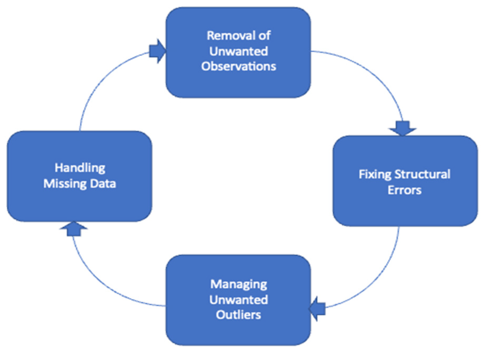
2.4. Data Preprocessing and Cleaning
- Rows with missing labels were dropped as they do not contribute to the learning process.
- Using the natural language toolkit (NLTK) library, tokenization was performed, i.e., tokens of the sentences were created.
- Stop words (if, then, the, and, etc.) were removed to keep only the text that would contribute to the learning process.
- Firstly, a regular expressions module was imported to help with data cleaning tasks. Regular expressions are sequences of characters that are used for matching with other strings in search. Patterns and strings of characters can be searched using regular expressions. Python has a “re” module that can help to find patterns and strings using regular expressions. Regular expressions can be used to remove or replace certain characters as part of data cleaning and preprocessing.
- Any newline characters or additional spaces were removed.
- Any URLs were also removed as they do not contribute to the learning process.
- Similarly, any other alphanumeric characters that included punctuation were removed for the same reason, including the following strings: !"#$%&\’()*+,-./:;<=>?@[\\]^_`{|}~. Only uppercase and lowercase letters along with digits 0–9 were kept.
- Stopwords such as “the”, “and”, “then”, and “if” were also removed as they are not a part of the learning process. Python’s NLTK library has stopwords in about 16 different languages. We imported English stopwords to remove them from our dataset. These words were removed as they do not add any additional information to the learning process.
- The outputs of these tasks were stored in a separate column, resulting in a column of tokenized words.
2.5. Tokenization, Sentence Padding, and Lemmatization
2.6. Simplification of Categorical Values
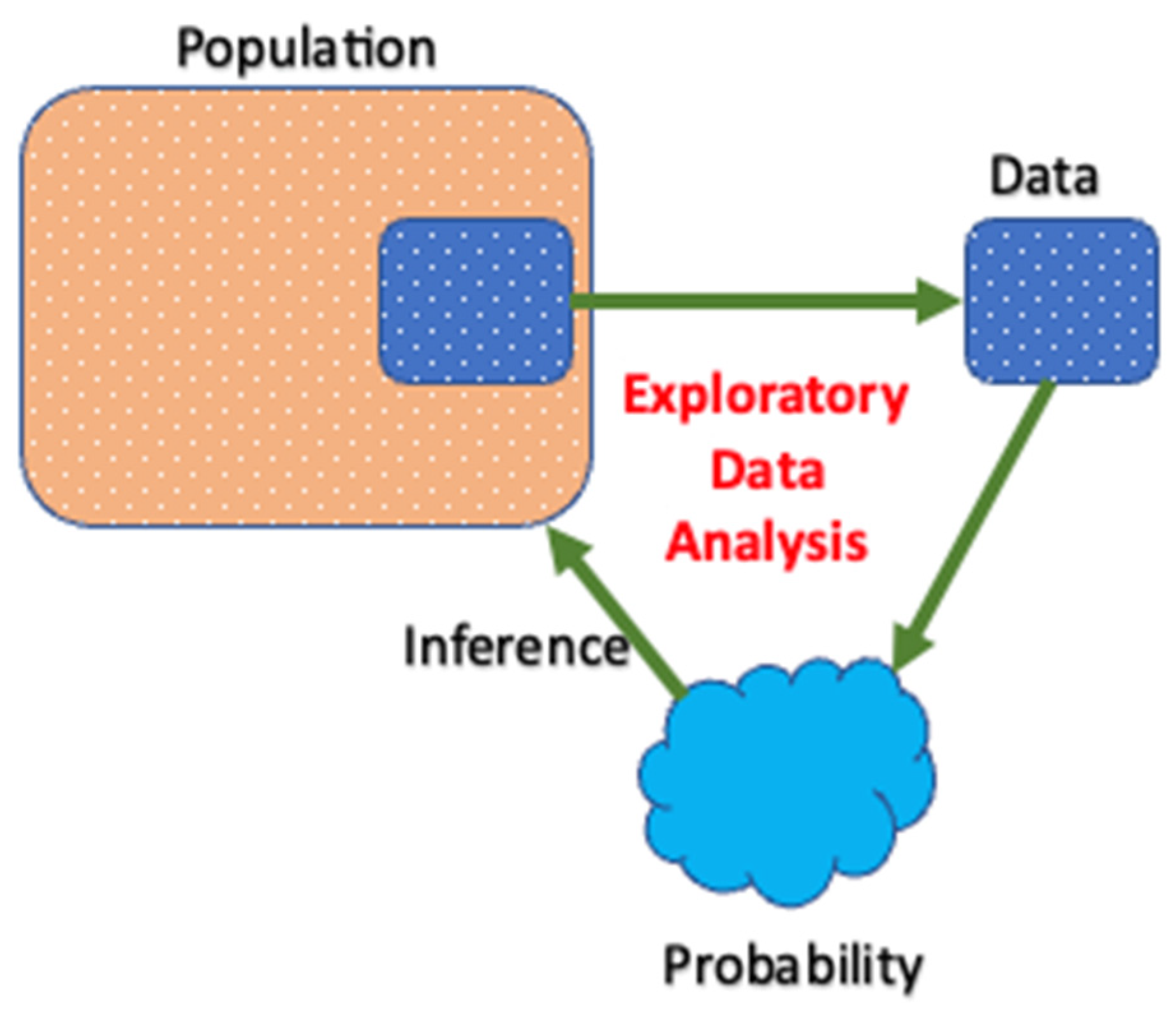
2.7. Exploratory Data Analysis (EDA)
2.8. Feature Extraction Methods
2.9. Classification Methods and Explainable Techniques
2.9.1. Deep Learning Model—Long Short-Term Memory (LSTM)
2.9.2. BERT (Bidirectional Encoder Representation from Transformers)
- Masked language model (MLM): In this task, BERT learns a featured representation for each of the words present in the vocabulary. About 85% of the words are used for training, and the remainder are used for evaluation. The selection of the training and evaluation sets is random and in iterations. Through this process, the model learns featured representation in a bidirectional way i.e., learns both the left and the right contexts of the words. In this task, some of the tokens from each sequence are replaced with the token [Mask]. The model is trained to predict these tokens using other tokens from sequence.
- Next sentence prediction (NSP): In this task, BERT learns the relationship between two different sentences. This task contributes to aspects such as question answering. The model is trained to predict the next sentence. It is similar to the textual entailment task where there are two sentences; it is a binary classification task to predict whether the second sentence succeeds the first sentence.
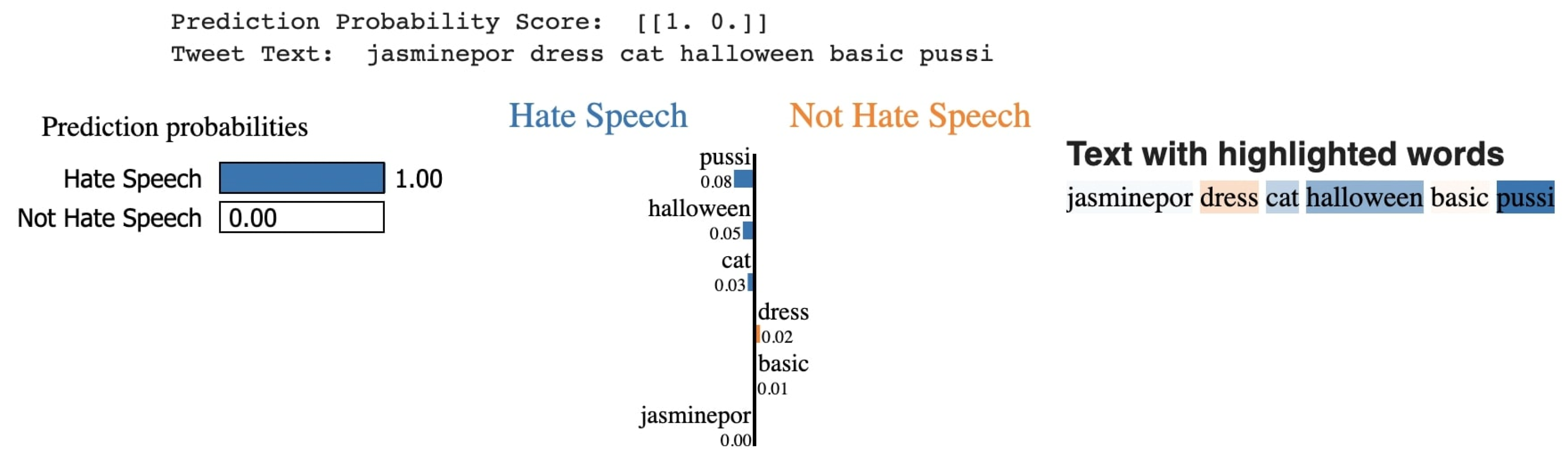
2.9.3. Local Interpretable Model—Agnostic Explanations (LIME)
3. Results
3.1. Model Training and Evaluation for Google Jigsaw Dataset
3.2. Model Training and Evaluation for HateXplain Dataset
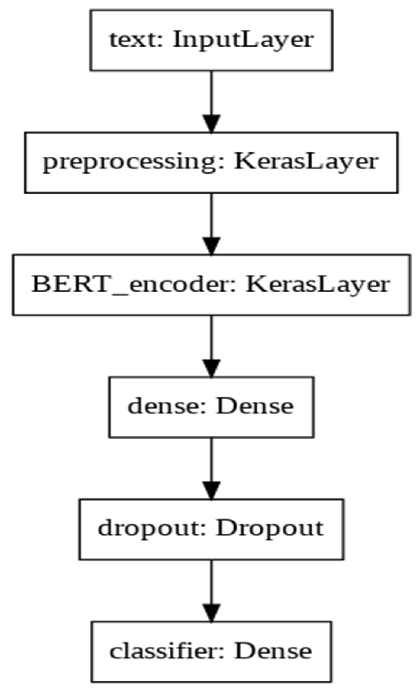
3.2.1. BERT + MLP
3.2.2. BERT + ANN
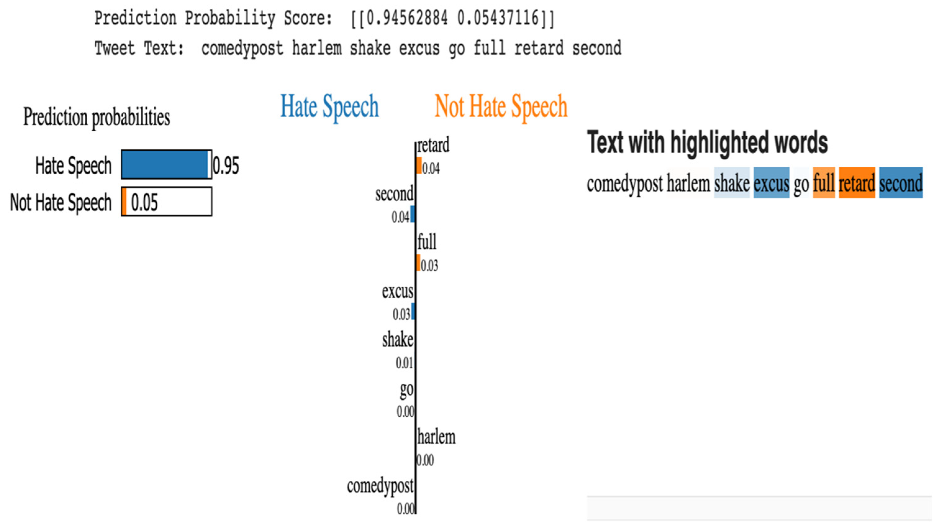
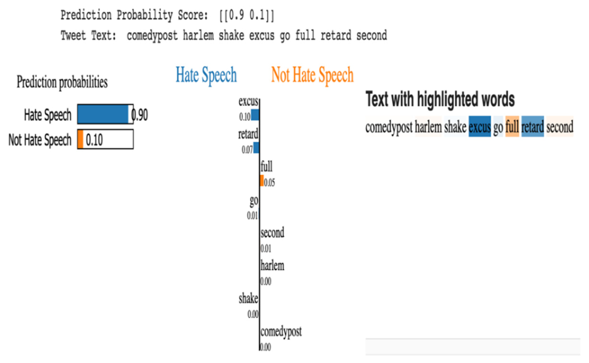
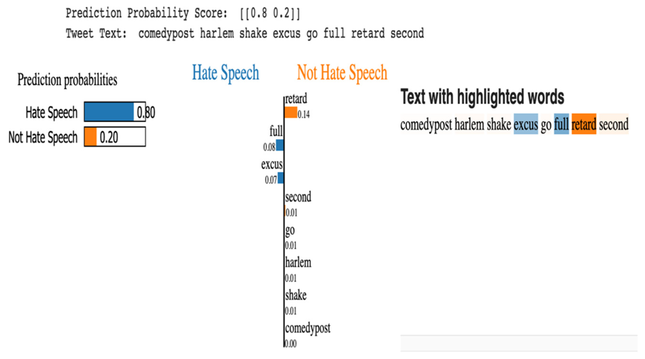
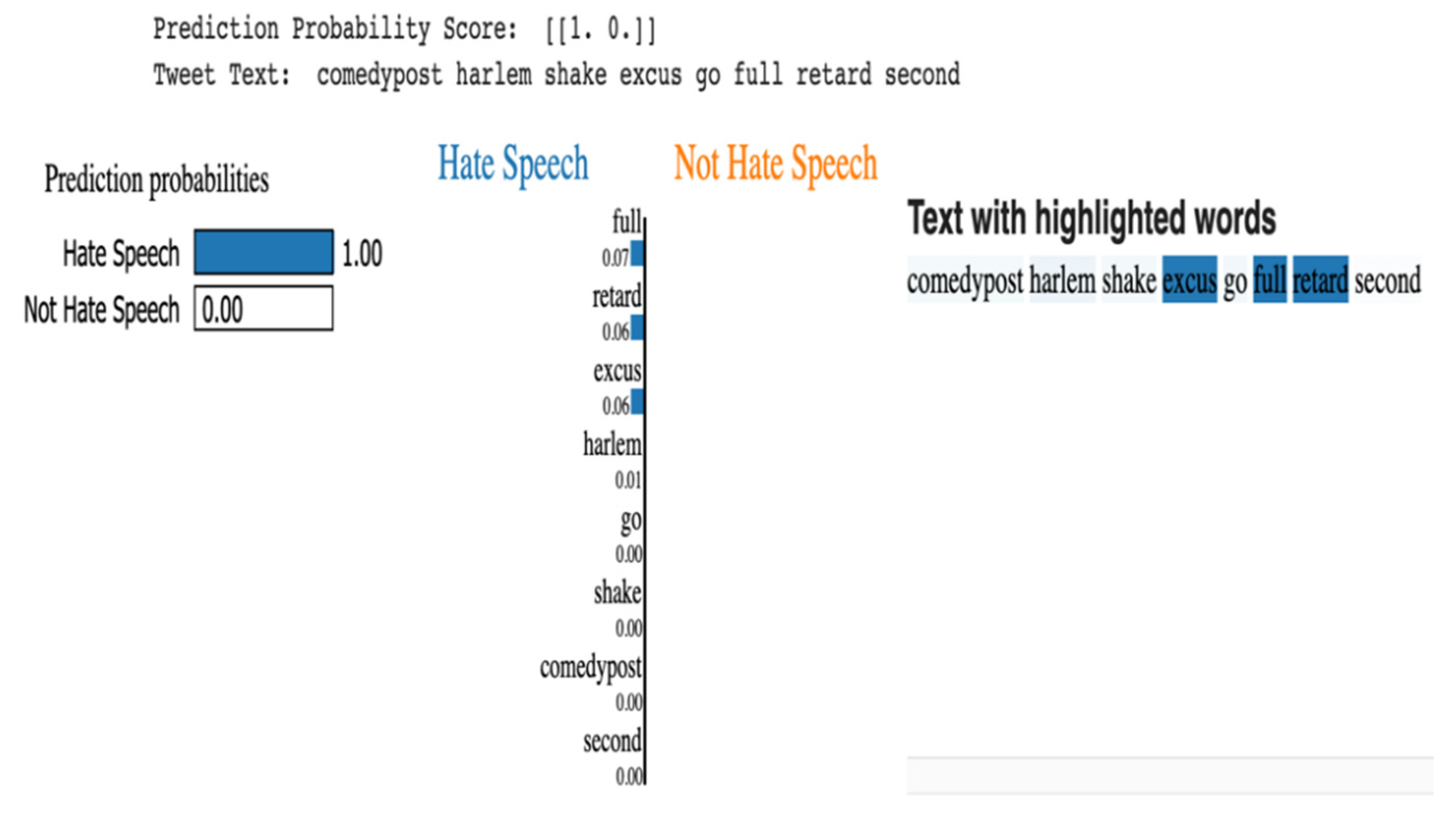
3.2.3. LIME with Machine Learning Models
Explainability with Random Forest
Explainability with Decision Tree
Explainability with Logistic Regression
3.2.4. Summary of Results for the HateXplain Dataset
Explainability Metrics
Bias-Based Metrics
4. Conclusions
4.1. Conclusions of the Study on the Google Jigsaw Dataset
4.2. Conclusion of the Study on the HateXplain Dataset
Author Contributions
Funding
Data Availability Statement
Conflicts of Interest
References
- Davidson, T.; Warmsley, D.; Macy, M.; Weber, I. Automated Hate Speech Detection and the Problem of Offensive Language. Available online: http://arxiv.org/abs/1703.04009 (accessed on 11 August 2022).
- Chen, Y.; Zhou, Y.; Zhu, S.; Xu, H. Detecting offensive language in social media to protect adolescent online safety. In Proceedings of the 2012 ASE/IEEE International Conference on Privacy, Security, Risk and Trust and 2012 ASE/IEEE International Conference on Social Computing, SocialCom/PASSAT, Amsterdam, The Netherlands, 3–5 September 2012; pp. 71–80. [Google Scholar] [CrossRef]
- Balkir, E.; Nejadgholi, I.; Fraser, K.C.; Kiritchenko, S. Necessity and sufficiency for explaining text classifiers: A case study in hate speech detection. arXiv 2022, arXiv:2205.03302. [Google Scholar]
- Chatzakou, D.; Kourtellis, N.; Blackburn, J.; de Cristofaro, E.; Stringhini, G.; Vakali, A. Mean birds: Detecting aggression and bullying on Twitter. In WebSci 2017—Proceedings of the 2017 ACM Web Science Conference; Association for Computing Machinery: New York, NY, USA, 2017; pp. 13–22. [Google Scholar] [CrossRef]
- Founta, A.M.; Chatzakou, D.; Kourtellis, N.; Blackburn, J.; Vakali, A.; Leontiadis, I. A Unified Deep Learning Architecture for Abuse Detection. In WebSci 2019—Proceedings of the 11th ACM Conference on Web Science; Association for Computing Machinery: New York, NY, USA, 2018; pp. 105–114. [Google Scholar] [CrossRef]
- Lundberg, S.M.; Lee, S.I. A unified approach to interpreting model predictions. Adv. Neural Inf. Process. Syst. 2017, 30. [Google Scholar]
- Arras, L.; Montavon, G.; Müller, K.R.; Samek, W. Explaining recurrent neural network predictions in sentiment analysis. In EMNLP 2017—8th Workshop on Computational Approaches to Subjectivity, Sentiment and Social Media Analysis, WASSA 2017—Proceedings of the Workshop; Association for Computational Linguistics: Copenhagen, Denmark, 2017. [Google Scholar] [CrossRef]
- Mahajan, A.; Shah, D.; Jafar, G. Explainable AI approach towards toxic comment classification. In Emerging Technologies in Data Mining and Information Security; Springer: Singapore, 2021; pp. 849–858. [Google Scholar]
- Ribeiro, M.T.; Singh, S.; Guestrin, C. “Why Should I Trust You?”: Explaining the Predictions of Any Classifier. In Proceedings of the NAACL-HLT 2016—2016 Conference of the North American Chapter of the Association for Computational Linguistics: Human Language Technologies, Proceedings of the Demonstrations Session, San Francisco, CA, USA, 13–17 August 2016; pp. 1135–1144. [Google Scholar] [CrossRef]
- Samek, W.; Montavon, G.; Lapuschkin, S.; Anders, C.J.; Müller, K.-R. Toward Interpretable Machine Learning: Transparent Deep Neural Networks and Beyond. Available online: https://doi.org/10.48550/arXiv.2003.07631 (accessed on 11 August 2022). [CrossRef]
- Doshi-Velez, F.; Kim, B. Towards A Rigorous Science of Interpretable Machine Learning. 2017. Available online: https://doi.org/10.48550/arXiv.1702.08608 (accessed on 11 January 2022). [CrossRef]
- Hind, M.; Wei, D.; Campbell, M.; Codella, N.C.F.; Dhurandhar, A.; Mojsilović, A.; Natesan Ramamurthy, K.; Varshney, K.R. TED: Teaching AI to explain its decisions. AIES 2019. In Proceedings of the 2019 AAAI/ACM Conference on AI, Ethics, and Society; Association for Computing Machinery: New York, NY, USA, 2019; pp. 123–129. [Google Scholar] [CrossRef]
- Montavon, G.; Samek, W.; Müller, K.-R. Methods for interpreting and understanding deep neural networks. Digit. Signal Process. 2018, 73, 1–15. [Google Scholar] [CrossRef]
- Gilpin, L.H.; Bau, D.; Yuan, B.Z.; Bajwa, A.; Specter, M.; Kagal, L. Explaining explanations: An overview of interpretability of machine learning. In Proceedings of the 2018 IEEE 5th International Conference on Data Science and Advanced Analytics, DSAA, Turin, Italy, 1–3 October 2018. [Google Scholar] [CrossRef]
- Lundberg, S.M.; Erion, G.; Chen, H.; DeGrave, A.; Prutkin, J.M.; Nair, B.; Katz, R.; Himmelfarb, J.; Bansal, N.; Lee, S. Explainable AI for Trees: From Local Explanations to Global Understanding. arXiv 2019, arXiv:1905.04610. Available online: http://arxiv.org/abs/1905.04610 (accessed on 11 May 2022). [CrossRef] [PubMed]
- Nori, H.; Jenkins, S.; Koch, P.; Caruana, R. InterpretML: A Unified Framework for Machine Learning Interpretability. arXiv 2019, arXiv:1909.09223. [Google Scholar] [CrossRef]
- Ahmed, U.; Lin, J.C.-W. Deep Explainable Hate Speech Active Learning on Social-Media Data. IEEE Trans. Comput. Soc. Syst. 2022, 1–11. [Google Scholar] [CrossRef]
- Barredo Arrieta, A.; Díaz-Rodríguez, N.; del Ser, J.; Bennetot, A.; Tabik, S.; Barbado, A.; Garcia, S.; Gil-Lopez, S.; Molina, D.; Benjamins, R.; et al. Explainable Artificial Intelligence (XAI): Concepts, taxonomies, opportunities and challenges toward responsible AI. Inf. Fusion 2020, 58, 82–115. [Google Scholar] [CrossRef]
- Das, A.; Rad, P. Opportunities and Challenges in Explainable Artificial Intelligence (XAI): A Survey. arXiv 2020, arXiv:2006.11371. [Google Scholar] [CrossRef]
- Kanerva, O. Evaluating Explainable AI Models for Convolutional Neural Networks with Proxy Tasks. Available online: https://www.semanticscholar.org/paper/Evaluating-explainable-AI-models-for-convolutional_Kanerva/d91062a3e13ee034af6807e1819a9ca3051daf13 (accessed on 25 January 2022).
- Gohel, P.; Singh, P.; Mohanty, M. Explainable AI: Current STATUs and Future Directions. Available online: https://doi.org/10.1109/ACCESS.2017 (accessed on 30 January 2022). [CrossRef]
- Fernandez, A.; Herrera, F.; Cordon, O.; Jose Del Jesus, M.; Marcelloni, F. Evolutionary fuzzy systems for explainable artificial intelligence: Why, when, what for, and where to? IEEE Comput. Intell. Mag. 2019, 14, 69–81. [Google Scholar] [CrossRef]
- Clinciu, M.-A.; Hastie, H. A Survey of Explainable AI Terminology. In Proceedings of the 1st Workshop on Interactive Natural Language Technology for Explainable Artificial Intelligence (NL4XAI 2019); Association for Computational Linguistics: Copenhagen, Denmark, 2019; pp. 8–13. [Google Scholar] [CrossRef]
- Hrnjica, B.; Softic, S. Explainable AI in Manufacturing: A Predictive Maintenance Case Study. In IFIP Advances in Information and Communication Technology, 592 IFIP; Springer: New York, NY, USA, 2020; pp. 66–73. [Google Scholar] [CrossRef]
- Miller, T. Explanation in artificial intelligence: Insights from the social sciences. Artif. Intell. 2019, 267, 1–38. [Google Scholar] [CrossRef]
- Mathew, B.; Saha, P.; Yimam, S.M.; Biemann, C.; Goyal, P.; Mukherjee, A. HateXplain: A Benchmark Dataset for Explainable Hate Speech Detection. arXiv 2020, arXiv:2012.10289. Available online: http://arxiv.org/abs/2012.10289 (accessed on 14 June 2021).
- ML|Overview of Data Cleaning. GeeksforGeeks. 15 May 2018. Available online: https://www.geeksforgeeks.org/data-cleansing-introduction/ (accessed on 3 April 2022).
- Pearson, R.K. Exploratory Data Analysis: A First Look. In Exploratory Data Analysis Using R; Chapman and Hall/CRC: New York, NY, USA, 2018. [Google Scholar]
- Using CountVectorizer to Extracting Features from Text. GeeksforGeeks. 15 July 2020. Available online: https://www.geeksforgeeks.org/using-countvectorizer-to-extracting-features-from-text/ (accessed on 3 April 2022).
- Bisong, E. The Multilayer Perceptron (MLP). In Building Machine Learning and Deep Learning Models on Google Cloud Platform; Apress: Berkeley, CA, USA, 2019; pp. 401–405. [Google Scholar] [CrossRef]
- Kamath, U.; Graham, K.L.; Emara, W. Bidirectional encoder representations from transformers (BERT). In Transformers for Machine Learning; Chapman and Hall/CRC: New York, NY, USA, 2022; pp. 43–70. [Google Scholar] [CrossRef]
- Awal, M.R.; Cao, R.; Lee, R.K.-W.; Mitrovic, S. AngryBERT: Joint Learning Target and Emotion for Hate Speech Detection. arXiv 2021, arXiv:2103.11800. Available online: http://arxiv.org/abs/2103.11800 (accessed on 16 July 2022).
- Nair, R.; Prasad, V.N.V.; Sreenadh, A.; Nair, J.J. Coreference Resolution for Ambiguous Pronoun with BERT and MLP. In Proceedings of the 2021 International Conference on Advances in Computing and Communications (ICACC), Kochi, India, 21–23 October 2021; pp. 1–5. [Google Scholar] [CrossRef]
- Biecek, P.; Burzykowski, T. Local interpretable model-agnostic explanations (LIME). In Explanatory Model Analysis; Chapman and Hall/CRC: New York, NY, USA, 2021; pp. 107–123. [Google Scholar] [CrossRef]
- DeYoung, J.; Jain, S.; Rajani, N.F.; Lehman, E.; Xiong, C.; Socher, R.; Wallace, B.C. ERASER: A Benchmark to Evaluate Rationalized NLP Models. arXiv 2020, arXiv:1911.03429. [Google Scholar] [CrossRef]


| Ref. | Contribution | Key Findings | Limitation(s) |
|---|---|---|---|
| [1] | Automated hate speech detection and the problem of offensive language | Logistic regression, naïve bayes, decision trees, random forests, and SVM are tested using 5-fold cross-validation | The definition of hate speech in this research is limited to language that threatens or incites violence which excludes a large proportion of hate speech. Lexical methods used are inaccurate at identifying hate speech, and only a small percentage of tweets flagged by hate base lexicon are considered hate speech. |
| [2] | Detection of offensive content and identification of potential offensive users | Lexical syntactical feature (LSF) framework | Comparison of existing text-mining methods in detecting offensive contents with LSF framework in not detailed and lacks scientific validation. |
| [3] | A feature attribution method for explainability | Necessity and sufficiency explained in detailed in the context of hate speech | The analysis is limited by limitation of the existing dataset used which lacks variety of demographic groups. |
| [4] | Detecting bullying and aggressive behavior on Twitter | Random forest classifier using WEKA tool, 10-fold cross-validation | Results obtained with random forest classifier are only presented with respect to training time and performance due to limited space. |
| [5] | A unified deep learning architecture for abuse detection | Deep learning architecture for detection of abuse online | Network-related metadata are not considered in the dataset due to time limitations as it takes a significant amount of computation to crawl Twitter data due to Twitter API rate limits. |
| [6] | A unified approach to explaining complex ML models | SHAP (Shapley additive explanations) framework for the explanation of complex, ensemble and deep learning models | SHAP model is not consistent with human intuition in some cases, which can lead to false positives or false negatives; a different approach is not considered in such cases. |
| [7] | Explanation of RNN predictions in sentiment analysis | Propagation rule for growing connections in recurrent neural networks (RNN) architectures | Gradient-based sensitivity analysis used with approach is not able to get accurate relevance score when a sentiment is decomposed into words. |
| [8] | Intuitive explainability along with using various deep learning techniques | LIME explanation with individual examples | Some misclassification is observed in the case of nontoxic comments. |
| [9] | Explaining the predictions of any classifier | LIME model to explain the predictions of any classifier, SP-LIME model for selecting representative and nonredundant explanations | The method to perform the pick-up step for images is not addressed in this research. |
| [10] | Interpretable machine learning models | Technical foundations of explainable artificial intelligence, presentation of practical XAI algorithms such as occlusion, integrated gradients, and LRP, importance, applications, challenges and directions for future work | The explanation revealed by model in this research are difficult to interpret by human observer due to limited accessibility of the data representation. Deeper understanding of relevance maps is not obtained by the model. |
| [11] | Evaluation of interpretability and explainability in machine learning | Application-grounded, human-grounded, and functionally grounded approaches for evaluation of interpretability, discussion of open questions related to these evaluation approaches | The research is focused only on the taxonomy to define and evaluate interpretability and not on methods to extract explanations. |
| [12] | Framework for the explanation of the results of an artificial intelligence system | Proposed framework named “teaching explanations for decisions (TED)” to provide explanations of an AI system | The proposed TED framework assumes a training dataset to be having explanation and applies cartesian product using any machine learning algorithm to train classifier instead of using multitask setting. |
| [13] | Explainability of deep neural network models | Key directions for moving towards transparency of machine learning models, novel technological development for explainability | This research does not focus on exact choice of deep neural network for any particular domain and instead is only focused on generalized conceptual developments. |
| [14] | Overview of interpretability of machine learning models | Need for diverse metrics for targeted explanations, suggestions for explainability of deep learning models | The study only focuses on abstract overview of explainability without diving deep into explanation metrics. |
| [15] | Enhancing interpretability of tree-based machine learning models | Method for computation of the game theoretic Shapley values, local explanation method, tools for explainability using a combination of local explanation methods | Only local explanations are presented that focuses on single samples without considering global explanations. |
| [16] | A unified framework for machine learning interpretability | An open-source package InterpretML for glass-box and blackbox explainability | Computational performance for models across datasets is not consistent for explainable boosting machine (EBM) model discussed in this research. |
| [17] | An active learning approach for labeling text | Attention network visualization for indirect and informal communication | The semantic embeddings and lexicon expansion techniques discussed in the paper lack detailed explanations. |
| [18] | Explainable artificial intelligence (XAI): categorization, contributions, suggestions, and issues in responsible AI | Overview of explainable artificial intelligence, literature review and taxonomy, implications, vision, and future of XAI | Some functions are proprietary and are not exposed to the public in this research. Explainable AI methods give explanations that are not aligned with what the original method calculates. |
| [19] | Opportunities and challenges in explainable artificial intelligence (XAI) | Survey on seminal algorithms for explainable deep neural network algorithms, evaluation of XAI methods and techniques | Human attention is not able to arrive at XAI explanation maps for decision making. Quantitative measures of completeness and correctness of the explanation map are not available |
| [20] | Evaluation of explainable artificial intelligence models for convolutional neural networks (CNN) with proxy tasks | Proposed two 2 proxy tasks, namely, pattern task and Gaussian blot task, which are then used to evaluate LIME, layer-wise relevance propagation, and Deep LIFT, and results are discussed | The evaluation scheme discussed in the research has issues with cross-model evaluation and is less comprehensive. |
| [21] | Discussion of various explainable AI techniques | Need for XAI, key issues in XAI, objectives and scope of XAI, survey on various XAI techniques and methodologies | The study focuses on XAI and its importance but fails to discuss the limitations of conventional AI and its combination with XAI. |
| [22] | Fuzzy systems for explainable artificial intelligence | Need, timeline, applications, and future work of fuzzy systems for XAI | The research fails to address how to arrive at a solution to the problems that are not measurable in the evolutionary fuzzy systems (EFS) patterns. |
| [23] | A literature survey on explainable artificial intelligence (XAI) terminology | Background, terminology, objectives of explainable artificial intelligence (XAI), natural language generation approach | The survey does not explain how to evaluate natural language generation (NLG). |
| [24] | Predictive maintenance case study based on explainable artificial intelligence (XAI) | A machine learning model based on a highly efficient gradient boosting decision tree is proposed for the prediction of machine errors or any tool failure. | Results of this research are presented using a generic dataset and not a real data; however, the presented concept shows high maturity with promising results. |
| [25] | Insights from social sciences related to explainable artificial intelligence (XAI) | Why questions are diversified in explainable AI, explanations are biased and social | Adopting the work of this research into explainable AI is not a straightforward step, and the models discussed need to be refined and extended to provide good exploratory agent. |
| Classification | Frequency |
|---|---|
| Clean | 201,081 |
| Toxic | 21,384 |
| Obscene | 12,140 |
| Insult | 11,304 |
| Identity hate | 2117 |
| Severe toxic | 1962 |
| Threat | 689 |
| Gab | Total | ||
|---|---|---|---|
| Hateful | 708 | 5227 | 5935 |
| Offensive | 2328 | 3152 | 5480 |
| Normal | 5770 | 2044 | 7814 |
| Undecided | 249 | 670 | 919 |
| Total | 9055 | 11,093 | 20,148 |
| Layer Type | Output Shape | # of Parameters |
|---|---|---|
| Embedding | (None, none, 128) | 3,840,000 |
| LSTM 1 | (None, none, 128) | 131,584 |
| LSTM 2 | (None, 128) | 131,584 |
| Dense | (None, 6) | 774 |
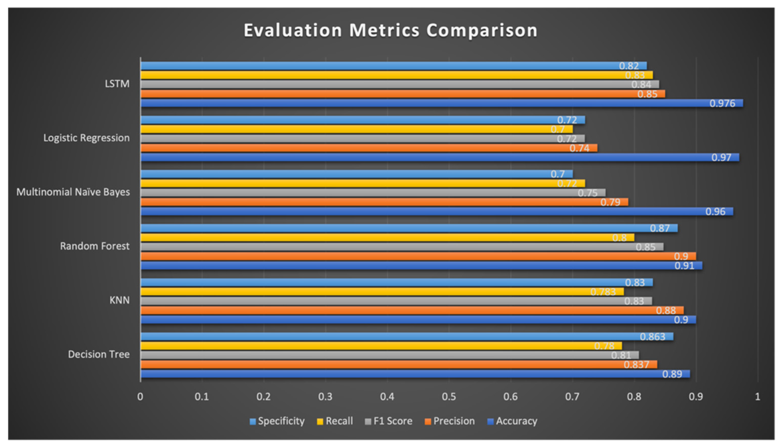
| Classifier Name | Accuracy | Precision | F1-Score | Sensitivity/Recall | Specificity |
|---|---|---|---|---|---|
| Decision Tree | 0.89 | 0.83 | 0.81 | 0.78 | 0.86 |
| K-nearest neighbors | 0.90 | 0.88 | 0.83 | 0.78 | 0.83 |
| Random forest | 0.91 | 0.90 | 0.85 | 0.80 | 0.87 |
| Multinomial naïve Bayes | 0.96 | 0.79 | 0.75 | 0.72 | 0.70 |
| Logistic regression | 0.97 | 0.74 | 0.72 | 0.70 | 0.72 |
| Long short-term memory (LSTM) | 0.97 | 0.85 | 0.84 | 0.83 | 0.82 |
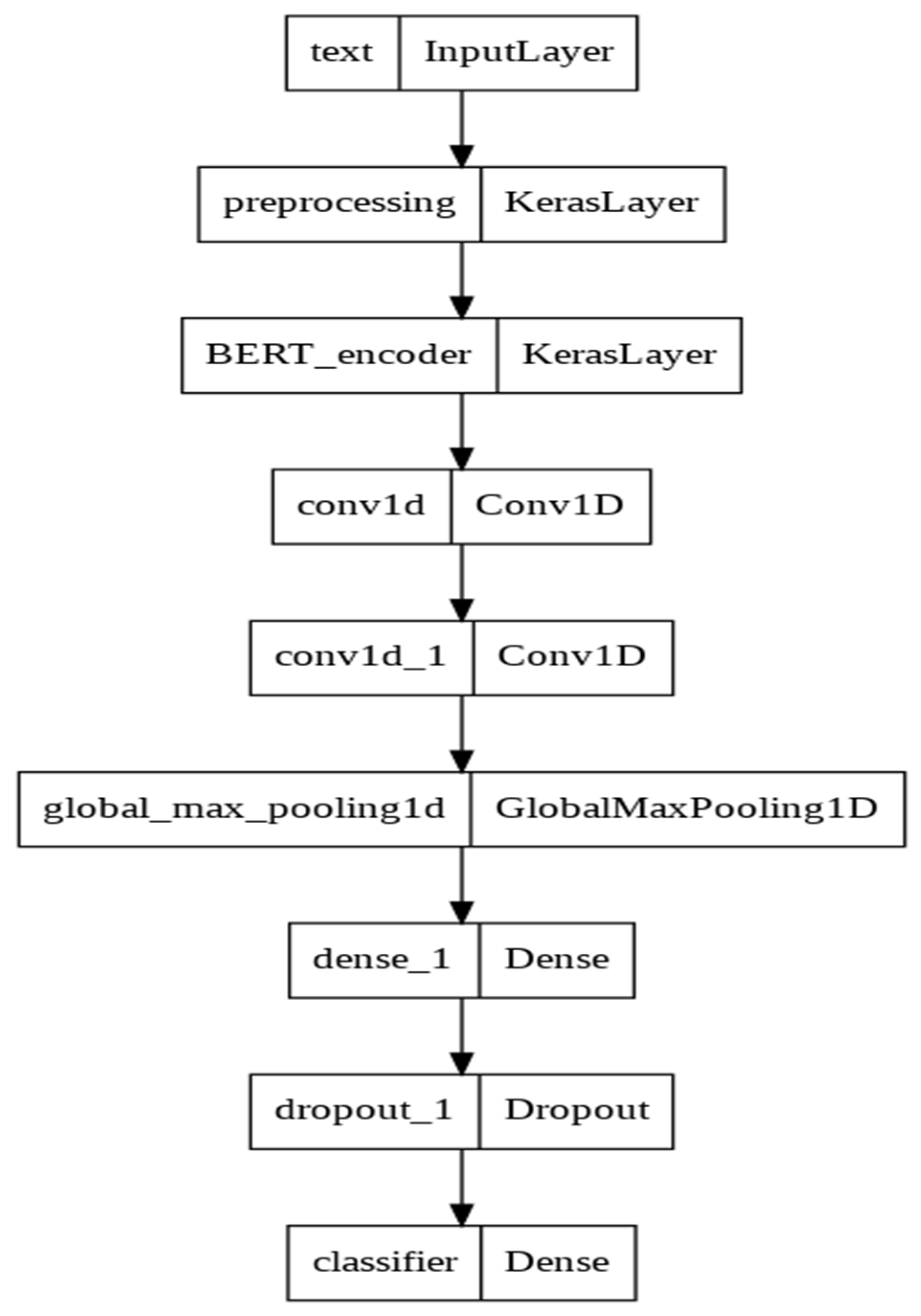
| Layer (Type) | Output Shape | # of Parameters | Connected to |
|---|---|---|---|
| text (InputLayer) | [(None,)] | 0 | [] |
| preprocessing (KerasLayer) | {‘input_word_ids’: (None,128), ‘input_mask’: (None, 128), ‘input_type_ids’: (None, 128)} | 0 | [‘text [0][0]’] |
| BERT_encoder (KerasLayer) | {‘pooled_output’: (28,763,649, None, 512), ‘encoder_outputs’: [(None, 128, 512), (None, 128, 512), (None, 128, 512), (None, 128, 512)], ‘default’: (None, 512), ‘sequence_output’: (None, 128, 512)} | 28,763,649 | [‘preprocessing [0][0]’, ‘preprocessing [0][1]’, ‘preprocessing [0][2]’,] |
| dense (Dense) | (None, 512) | 262,656 | [‘BERT_encoder [0][5]’] |
| dropout (Dropout) | (None, 512) | 0 | [‘dense [0][0]’] |
| classifier (Dense) | (None, 3) | 1539 | [‘dropout [0][0]’] |
| Total params: 29,027,844 | |||
| Trainable params: 29,027,843 | |||
| Non-trainable params: 1 | |||
| Layer (Type) | Output Shape | # of Parameters | Connected to |
|---|---|---|---|
| text (InputLayer) | [(None,)] | 0 | [] |
| preprocessing (KerasLayer) | {‘input_word_ids’:(None,128), ‘input_mask’: (None, 128), ‘input_type_ids’: (None, 128)} | 0 | [‘text [0][0]’] |
| BERT_encoder (KerasLayer) | {‘pooled_output’: (28,763,649, None, 512), sequence_outputs’: (None, 128, 512), ‘encoder_outputs’: [(None, 128, 512), (None, 128, 512), (None, 128, 512), (None, 128, 512)], ‘default’: (None, 512), ‘sequence_output’: (None, 128, 512)} | 28,763,649 | [‘preprocessing [0][0]’, ‘preprocessing [0][1]’, ‘preprocessing [0][2]’,] |
| Conv1d (Conv1D) | (None, 127, 32) | 32,800 | [‘BERT_encoder [0][6]’] |
| Conv1d_1 (Conv1D) | (None, 126, 64) | 4160 | [‘conv1d [0][0]’] |
| Global_max_pooling1d (GlobalMaxpooling1D) | (None, 64) | 0 | [‘conv1d_1 [0][0]’] |
| dense_1 (Dense) | (None, 512) | 33,280 | [‘BERT_encoder [0][5]’] |
| dropout_1 (Dropout) | (None, 512) | 0 | [‘dense_1 [0][0]’] |
| classifier (Dense) | (None, 3) | 1539 | [‘dropout_1 [0][0]’] |
| Total params: 28,835,428 | |||
| Trainable params: 28,835,427 | |||
| Non-trainable params: 1 | |||
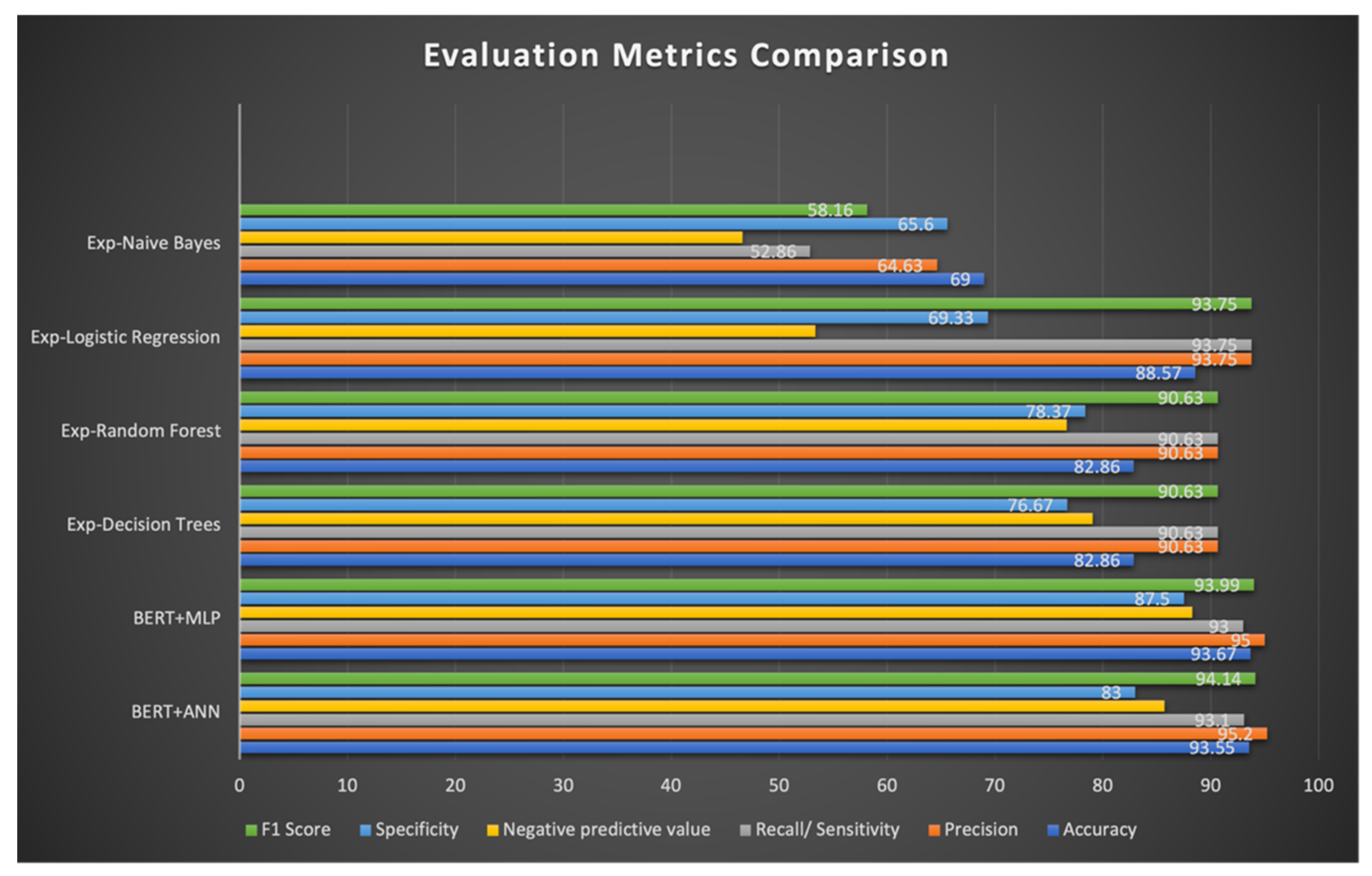
| S. No | Full Form | Features | Accuracy | Precision | Recall/Sensitivity | Negative Predictive Value | Specificity | F1-Score |
|---|---|---|---|---|---|---|---|---|
| 1 | Bidirectional encoder representations from transformers + artificial neural network layers (BERT + ANN) | Explainable, layer-wise propagation | 93.55 | 95.2 | 93.1 | 85.7 | 83 | 94.14 |
| 2 | Bidirectional encoder representations from transformers + multilayer perceptron (BERT + MLP) | Explainable, layer-wise propagation | 93.67 | 95 | 93 | 88.3 | 87.5 | 93.99 |
| 3 | Exp-decision trees | Explainable (LIME) | 82.86 | 90.63 | 90.63 | 79.03 | 76.67 | 90.63 |
| 4 | Exp-random forest | Explainable (LIME) | 82.86 | 90.63 | 90.63 | 76.65 | 78.37 | 90.63 |
| 5 | Exp-logistic regression | Explainable (LIME) | 88.57 | 93.75 | 93.75 | 53.33 | 69.33 | 93.75 |
| 6 | Exp-naïve Bayes | Explainable (LIME) | 69 | 64.63 | 52.86 | 46.6 | 65.6 | 58.16 |
| Technique | Plausibility | Faithfulness | |||
|---|---|---|---|---|---|
| IOU F1 | Token F1 | AUPRC | Comprehensiveness | Sufficiency | |
| BERT + ANN | 0.1888 | 0.5074 | 0.8384 | 0.4199 | 0.0055 |
| BERT + MLP | 0.298 | 0.5298 | 0.8589 | 0.3574 | 0.003 |
| DT-LIME | 0.1676 | 0.3887 | 0.7487 | 0.2993 | 0.0442 |
| RF-LIME | 0.2387 | 0.5118 | 0.8469 | 0.4132 | 0.0014 |
| LR-LIME | 0.1008 | 0.2271 | 0.5284 | 0.2132 | 0.0482 |
| NB-LIME | 0.1287 | 0.1818 | 0.5938 | 0.1999 | 0.0514 |
| Technique | Subgroup AUC | BPSN AUC | BSNP AUC |
|---|---|---|---|
| BERT + ANN | 0.7977 | 0.7188 | 0.7391 |
| BERT + MLP | 0.8229 | 0.7752 | 0.8077 |
| DT-LIME | 0.6926 | 0.6578 | 0.6617 |
| RF-LIME | 0.7627 | 0.6977 | 0.5978 |
| LR-LIME | 0.5266 | 0.4522 | 0.4991 |
| NB-LIME | 0.6136 | 0.4812 | 0.5049 |
Publisher’s Note: MDPI stays neutral with regard to jurisdictional claims in published maps and institutional affiliations. |
© 2022 by the authors. Licensee MDPI, Basel, Switzerland. This article is an open access article distributed under the terms and conditions of the Creative Commons Attribution (CC BY) license (https://creativecommons.org/licenses/by/4.0/).
Share and Cite
Mehta, H.; Passi, K. Social Media Hate Speech Detection Using Explainable Artificial Intelligence (XAI). Algorithms 2022, 15, 291. https://doi.org/10.3390/a15080291
Mehta H, Passi K. Social Media Hate Speech Detection Using Explainable Artificial Intelligence (XAI). Algorithms. 2022; 15(8):291. https://doi.org/10.3390/a15080291
Chicago/Turabian StyleMehta, Harshkumar, and Kalpdrum Passi. 2022. "Social Media Hate Speech Detection Using Explainable Artificial Intelligence (XAI)" Algorithms 15, no. 8: 291. https://doi.org/10.3390/a15080291
APA StyleMehta, H., & Passi, K. (2022). Social Media Hate Speech Detection Using Explainable Artificial Intelligence (XAI). Algorithms, 15(8), 291. https://doi.org/10.3390/a15080291