Discrete-Time Observations of Brownian Motion on Lie Groups and Homogeneous Spaces: Sampling and Metric Estimation

Abstract

We present schemes for simulating Brownian bridges on complete and connected Lie groups and homogeneous spaces. We use this to construct an estimation scheme for recovering an unknown left- or right-invariant Riemannian metric on the Lie group from samples. We subsequently show how pushing forward the distributions generated by Brownian motions on the group results in distributions on homogeneous spaces that exhibit a non-trivial covariance structure. The pushforward measure gives rise to new non-parametric families of distributions on commonly occurring spaces such as spheres and symmetric positive tensors. We extend the estimation scheme to fit these distributions to homogeneous space-valued data. We demonstrate both the simulation schemes and estimation procedures on Lie groups and homogenous spaces, including $SPD\left(3\right)={\mathrm{GL}}_{+}\left(3\right)/\mathrm{SO}\left(3\right)$ and ${\mathbb{S}}^2=\mathrm{SO}\left(3\right)/\mathrm{SO}\left(2\right)$.

1. Introduction

Bridge simulation is a data augmentation technique for generating missing trajectories of continuous diffusion processes. We consider bridge simulation on Lie groups and homogeneous spaces. As an important example, we investigate the case of an i.i.d. Lie group or homogeneous space-valued samples that are considered discrete-time observations of a continuous diffusion process. Assuming the stochastic dynamics to be Brownian motion, we wish to estimate the underlying Riemannian metric of the Lie group or homogeneous space from the samples. To evaluate and maximize the likelihood of the data, we need to account for the diffusion process being unobserved at most time points. This requires bridge sampling, and the sampling techniques are thus the key enabler for metric estimation in this setting.

The simulation of conditioned diffusion processes is a highly non-trivial problem, even in Euclidean spaces. Transition densities of diffusion processes are tractable in closed form only for a small class of processes, and hence, simulating directly from the true bridge distribution is generally infeasible. The data augmentation used in inference for diffusion processes dates back to the seminal paper by Pedersen [1] almost three decades ago. Since then, several papers have studied diffusion bridge simulation methods; see, e.g., [2,3,4,5,6,7,8,9,10,11]. The method by Delyon and Hu [5] exchanged the intractable drift term in the conditioned diffusion with a tractable drift originating from the drift of a standard Brownian bridge.

In this paper, we further extend the original idea of Delyon and Hu [5] to Lie groups and homogenous spaces. Several papers have built on the ideas of Delyon and Hu. For example, a manifold equivalent drift term analogous to the drift term of a Brownian bridge in Euclidean space was used in [6] to describe the simulation of Brownian bridges on the flat torus, whereas [7] generalized this method to general finite-dimensional Riemannian manifolds. Reference [11] used the drift to model Brownian bridges on the space of landmarks. Bui et al. [4,12] used a similar drift term on the space of symmetric positive definite (covariance) matrices, exploiting the exponential map, which in the space of covariance matrices is a global diffeomorphism. The present paper extends these ideas to general Lie groups and homogeneous spaces.

As an application, we consider discrete-time observations in Lie groups and homogeneous spaces regarded as incomplete observations of sample paths of Brownian motions arising from left- (or right-) invariant Riemannian metrics. The bridge simulation schemes allow interpolating between the discrete-time observations. Furthermore, we observe how varying the metric on Lie groups affects pushforwards of the Brownian motion to homogeneous spaces being quotients of the group. These distributions encode the covariance of the data resulting from the metric structure of the Lie group. We define this family of distributions and derive estimation schemes for recovering the metric structure of the group both with Lie group samples and with homogeneous space samples. One particular example is the two-sphere, ${\mathbb{S}}^2\cong \mathrm{SO}\left(3\right)/\mathrm{SO}\left(2\right)$. Changing the metric structure on $\mathrm{SO}\left(3\right)$ results in anisotropic distributions on ${\mathbb{S}}^2$, arising as the pushforward measure from $\mathrm{SO}\left(3\right)$. Figure 1 illustrates the isotropic and anisotropic distributions on ${\mathbb{S}}^2$ induced by a bi-invariant and left-invariant (not bi-invariant) metric on $\mathrm{SO}\left(3\right)$, respectively. The resulting distributions are analogous to the von Mises–Fisher and Fisher–Bingham–Kent distributions [13,14]. However, the approach is independent of the chosen embedding and uses only the geometric relation between the group and quotient space.

Figure 1. The two leftmost plots visualize the transition densities of (a) a Fisher–Bingham–Kent distribution and (b) the pushforward density of a Brownian motion to ${\mathbb{S}}^2$ with a bi-invariant metric. The pushforward measure of a Brownian motion on $\mathrm{SO}\left(3\right)$ to the sphere ${\mathbb{S}}^2$ results in anisotropic distributions on ${\mathbb{S}}^2$ when the metric on $\mathrm{SO}\left(3\right)$ is not bi-invariant, for (c) $T=0.5$ and (d) $T=1.0$. The coloring indicates the density of the pushforward (different color scheme for each subfigure).

For the simulation on homogeneous spaces, we use bridges to submanifolds as developed by Thompson [15] to condition on the fibers in the Lie group G over the target point $v\in M=G/H$ for some closed subgroup $H\subset G$. The resulting guiding term guides in the direction closest to the fiber.

Statistics on Lie groups and homogeneous spaces find applications in many diverse fields, including bioinformatics, medical imaging, shape analysis, computer vision, and information geometry; see, e.g., [16,17,18,19,20]. Statistics in Euclidean spaces often rely on the distributional properties of the normal distribution. Here, we use Brownian motions and the heat equation to generalize the normal distribution to Lie groups and homogeneous spaces as introduced by Grenander [21]. The solution to the heat equation is the transition density of a Brownian motion. Through Monte Carlo simulations of bridges, we can estimate the transition density and maximize the likelihood with respect to the Riemannian metric.

Contribution and Overview

We present simulation schemes on Lie groups and homogeneous spaces with application to parameter estimation. We outline the necessary theoretical background for the construction of bridge simulation on Lie groups and homogeneous spaces before demonstrating how the simulation scheme leads to estimates of means and the underlying metric structure using maximum likelihood estimation on certain Lie groups and homogeneous spaces. The paper builds on and significantly extends the conference paper [22], which introduced bridge simulation in the Lie group setting.

The paper is organized as follows: In Section 2, we describe the relevant background theory of Lie groups, Brownian motions, and Brownian bridges in Riemannian manifolds. Section 3 presents the theory and results of bridge sampling in Lie groups, and Section 4 introduces bridge sampling on homogeneous spaces. Section 5 covers maximum likelihood estimation of the starting point and Riemannian metric. Numerical experiments on selected Lie groups and homogeneous spaces are presented in Section 6.

2. Notation and Background

We here briefly describe simulating conditioned diffusions in Euclidean space as developed in [5] before reviewing the theory on conditioned diffusions on Riemannian manifolds.

2.1. Euclidean Diffusion Bridges and Simulation

Suppose a strong solution exists to an SDE of the form

$$\begin{array}{c}\hfill d{x}_t=b(t,x_t)dt+\sigma (t,x_t)d{w}_t,\end{array}$$

where b and $\sigma$ satisfy certain regularity conditions and where w denotes an ${\mathbb{R}}^n$-valued Brownian motion. In this case, x is a Markov process, and its transition density exists. Suppose we define the function

$$\begin{array}{c}\hfill h(t,x)=\frac{p_{T-t}(x_t,v)}{p_T(x_0,v)},\end{array}$$

for some $x_0,v\in {\mathbb{R}}^n$. Then, it is easily derived that h is a martingale on $[0,T)$ with $h(0,x_0)=1$, and Doob’s h-transform implies that the SDE of the conditioned diffusion $x|x_T=v$ is given by

$$\begin{array}{c}\hfill d{y}_t=\tilde{b}(t,y_t)dt+\sigma (t,y_t)d{w}_t\end{array}$$

where $\tilde{b}(t,y)=b(t,y)+\left(\sigma {\sigma }^T\right)(t,y){\nabla }_{y}log{p}_{T-t}(y,v)$. In the case that the transition density is intractable, simulation from the exact distribution is infeasible. Delyon and Hu [5] suggested substituting the latter term in $\tilde{b}$ with a drift term of the form $-(y_t-v)/(T-t)$, which equals the drift term in a Brownian bridge. The guided process obtained by making the above substitution yields a conditioning, and one obtains

$$\mathbb{E}\left[f\left(x\right)\right|x_T=v]=C\mathbb{E}\left[f\left(y\right){\phi }_T\left(y\right)\right],$$

(1)

where ${\phi }_T$ is a likelihood function that is tractable and numerically computable, y is the guided process, and the constant $C>0$ depends on $x_0$, v, and T.

2.2. Riemannian Manifolds and Lie Groups

Let M be a finite-dimensional smooth manifold of dimension d. M can be endowed with a Riemannian metric tensor, i.e., a family of inner products ${\left\{{⟨·,·⟩}_x\right\}}_{x\in M}$ defined on each tangent space $T_{x}M$. The Riemannian metric tensor gives rise to a distance function between points in M. The tangent space is locally diffeomorphic with an open subset of M. The Riemannian exponential map ${Exp}_x: T_{x}M\to M$ provides this local diffeomorphism. On the subset of M where ${Exp}_x$ is a diffeomorphism, the inverse Riemannian exponential map, also called the Riemannian logarithm map, ${Log}_x: M\to T_{x}M$ is defined. The Riemannian distance function can then be defined in terms of the Riemannian inner product as $d(x,y)={\parallel {Log}_x\left(y\right)\parallel }_x$. The Riemannian logarithm map plays an important role when defining guided bridges on manifolds.

Let X be a vector field on M assigning to each point $X\in M$ a tangent vector $X\left(x\right)\in T_{x}M$. A connection ∇ on a manifold is an operation that allows us to compare neighboring tangent spaces and define derivatives of vector fields along other vector fields, that is, if Y is another vector field, then ${\nabla }_{X}Y$ is the derivative of Y along X (also known as the covariant derivative of Y along X). A connection also gives a notion of “straight lines” in manifolds, also known as geodesics. A curve $\gamma$ is a geodesic if the vector field along $\gamma$ is parallel to itself, i.e., if ${\nabla }_{{\dot{\gamma }}_t}{\dot{\gamma }}_t=0$. The geodesic curves are locally length minimizing.

Generalizing the Euclidean Laplacian operator, the Laplace–Beltrami operator is defined as the divergence of the gradient, ${\Delta }_{M}f=divgradf$. In terms of local coordinates $(x_1,\cdots ,x_d)$, the expression for the Laplace–Beltrami operator becomes

$$\begin{array}{c}\hfill {\Delta }_{M}f=det{\left(g\right)}^{-1/2}\left(\frac{\partial }{\partial x_j}{g}^{ji}det{\left(g\right)}^{1/2}\frac{\partial }{\partial x_i}\right)f,\end{array}$$

(2)

where $det\left(g\right)$ denotes the determinant of the Riemannian metric g and $g^{ij}$ are the coefficients of the inverse of g. (2) can be written as

$$\begin{array}{cc}\hfill {\Delta }_{M}f& =a^{ij}\frac{\partial }{\partial x_i}\frac{\partial }{\partial x_j}f+b^j\frac{\partial }{\partial x_j}f,\hfill \end{array}$$

(3)

where $a^{ij}=g^{ij}$, $b^k=-g^{ij}{\Gamma }_{ij}^k$, and $\Gamma$ denote the Christoffel symbols of the Riemannian metric.

2.3. Lie Groups

Let G denote a connected Lie group of dimension d, i.e., a smooth manifold with a group structure such that the group operations $G\times G\ni (x,y)\stackrel{\mu }{\mapsto }xy\in G$ and $G\ni x\stackrel{\iota }{\mapsto }{x}^{-1}\in G$ are smooth maps. If $x\in G$, the left-multiplication map, $L_{x}y$, defined by $y\mapsto \mu (x,y)$, is a diffeomorphism from G to itself. Similarly, the right-multiplication map $R_{x}y$ defines a diffeomorphism from G to itself by $y\mapsto \mu (y,x)$. Let $d{L}_x:TG\to TG$ denote the pushforward map given by ${\left(d{L}_x\right)}_y:T_{y}G\to T_{xy}G$. A vector field V on G is said to be left-invariant if ${\left(d{L}_x\right)}_{y}V\left(y\right)=V\left(xy\right)$. The space of left-invariant vector fields is linearly isomorphic to $T_{e}G$, the tangent space at the identity element $e\in G$. By equipping the tangent space $T_{e}G$ with the Lie bracket, we can identify the Lie algebra $\mathfrak{g}$ with $T_{e}G$. The group structure of G makes it possible to define an action of G on its Lie algebra $\mathfrak{g}$. The conjugation map $C_x:=L_x\circ R_x^{-1}:y\mapsto xy{x}^{-1}$, for $x\in G$, fixes the identity e. Its pushforward map at e, ${\left(d{C}_x\right)}_e$, is then a linear automorphism of $\mathfrak{g}$. Define $Ad\left(x\right):={\left(d{C}_x\right)}_e$, then $Ad:x\mapsto Ad\left(x\right)$ is the adjoint representation of G in $\mathfrak{g}$. The map $G\times \mathfrak{g}\ni (x,v)\mapsto Ad\left(x\right)v\in \mathfrak{g}$ is the adjoint action of G on $\mathfrak{g}$. We denote by $⟨·,·⟩$ a Riemannian metric on G. The metric is said to be left-invariant if ${⟨u,v⟩}_y={⟨{\left(d{L}_x\right)}_{y}u,{\left(d{L}_x\right)}_{y}v⟩}_{L_x\left(y\right)}$, for every $u,v\in T_{y}G$, i.e., the left-multiplication maps are isometries, for every $x\in G$. The metric is $Ad\left(G\right)$-invariant if ${⟨u,v⟩}_e={⟨Ad\left(x\right)u,Ad\left(x\right)v⟩}_e$, for every $u,v\in \mathfrak{g}$. Note that an $Ad\left(G\right)$-invariant metric on G is equivalent to a bi-invariant (left- and right-invariant) inner product on $\mathfrak{g}$. The differential of the Ad map at the identity yields a linear map $Ad\left(x\right)=\frac{d}{dt}{Ad(exp\left(tx\right))|}_0$. This linear map is equal to the Lie bracket $[v,w]=Ad\left(v\right)w$, $v,w\in \mathfrak{g}$.

A one-parameter subgroup of G is a continuous homomorphism $\gamma :(\mathbb{R},+)\to G$. The Lie group exponential map $exp:\mathfrak{g}\to G$ is defined as $exp\left(v\right)={\gamma }_v\left(1\right)$, for $v\in \mathfrak{g}$, where ${\gamma }_v$ is the unique one-parameter subgroup of G whose tangent vector at e is v. For matrix Lie groups, the exponential map has the particular form: $exp\left(A\right)={\sum }_{k=0}^{\infty }{A}^k/k!$, for a square matrix A. The resulting matrix $exp\left(A\right)$ is an invertible matrix. Given an invertible matrix B, if there exists a square matrix A such that $B=exp\left(A\right)$, then A is said to be the logarithm of B. In general, the logarithm might not exist, and if it does, it may fail to be unique. In a neighborhood sufficiently close to the identity, the Lie group logarithm exists and is unique. By means of left-translation (or right-translation), the Lie group exponential map can be extended to a map ${exp}_g:T_{g}G\to G$, for all $g\in G$, defined by ${exp}_g\left(v\right)=gexp\left(d{L}_{g^{-1}}v\right)$. Similarly, the Lie group logarithm at g becomes ${log}_g\left(v\right)=d{L}_{g}log\left(g^{-1}v\right)$. The matrix exponential and logarithms can be computed numerically efficiently (see [23], Chapter 5, and the references therein).

Example 1.

A few examples of Lie groups include the Euclidean space $({\mathbb{R}}^n,+)$ with the additive group structure, $({\mathbb{R}}_{+},·)$ the positive real line with a multiplicative group structure, the space of invertible real matrices $\mathrm{GL}\left(n\right)$ equipped with a multiplication of matrices forming a Lie group, and the rotation group $\mathrm{O}\left(n\right)$, consisting of real orthogonal matrices with determinant one or minus one forming a subgroup of $\mathrm{GL}\left(n\right)$.

The identification of the space of left-invariant vector fields with the Lie algebra $\mathfrak{g}$ allows for a global description of ${\Delta }_G$. Indeed, let $\{v_1,\cdots v_d\}$ be an orthonormal basis of $T_{e}G$. Then, $V_i\left(g\right)={\left(d{L}_g\right)}_e{v}_i$ defines left-invariant vector fields on G and the Laplace–Beltrami operator can be written as (cf. [24], Proposition 2.5)

$${\Delta }_{G}f\left(e\right)=\sum _{i=1}^d{V}_i^{2}f\left(e\right)-V_{0}f\left(e\right),$$

where $V_0={\sum }_{i,j=1}^d{C}_{ij}^j{V}_j$ and $C_{ij}^k$ denote the structure coefficients given by

$$[V_i,V_j]=C_{ij}^k{V}_k.$$

(4)

By left-invariance, ${\Delta }_{G}f\left(g\right)={\Delta }_{G}f\circ L_g\left(e\right)={\left(d{L}_g\right)}_e{\Delta }_{G}f\left(e\right)$.

2.4. Homogeneous Spaces

A homogeneous space is a particular type of quotient manifold that arises as a smooth manifold endowed with a transitive smooth action by a Lie group G. The homogeneous space is called a G-homogeneous space to indicate the Lie group action. All G-homogeneous spaces arise as a quotient manifold $G/H$, for some closed subgroup $H\subseteq G$. H is a closed subgroup of the Lie group G, which makes H a Lie group. Any homogeneous space is diffeomorphic to the quotient space $G/G_x$, where $G_x$ is the stabilizer for the point x. The dimension of the G-homogeneous space is equal to $dimG-dimH$; the quotient map $\pi :G\to G/H$ is a smooth submersion, i.e., the differential of $\pi$ is surjective at every point. This implies that the fibers ${\pi }^{-1}\left(x\right)$, $x\in M$, are embedded submanifolds of G. We assume throughout that G acts on itself by left-multiplication.

Example 2.

The rotation group $\mathrm{SO}\left(n\right)$ acts transitively on ${\mathbb{S}}^{n-1}$; therefore, ${\mathbb{S}}^{n-1}$ is an $\mathrm{SO}\left(n\right)$-homogeneous space. Consider a point in ${\mathbb{S}}^{-1}$ as a vector in ${\mathbb{R}}^n$. Rotations that fix the point occur precisely in the subspace orthogonal to the vector. Thus, the stabilizer or isotropy group is the rotation group $\mathrm{SO}(n-1)$ and ${\mathbb{S}}^{n-1}=\mathrm{SO}\left(n\right)/\mathrm{SO}(n-1)$. The set of invertible matrices with positive determinant ${\mathrm{GL}}_{+}\left(n\right)$ acts on symmetric positive definite matrices $SPD\left(n\right)$. The isotropy group is the rotation group $\mathrm{SO}\left(n\right)$, and thus, $SPD\left(n\right)={\mathrm{GL}}_{+}\left(n\right)/\mathrm{SO}\left(n\right)$. A particular type of homogeneous space arises when the subgroup is a discrete subgroup of G. For example, the space ${\mathbb{T}}^n={\mathbb{R}}^n/{\mathbb{Z}}^n$ defines the n-torus as a homogeneous space.

2.5. Brownian Motion on Riemannian Manifolds

The Laplacian defines Brownian motion on M as a $\frac{1}{2}{\Delta }_M$-diffusion process up to its explosion time $\tau$. The stochastic differential equation (SDE) for a Brownian motion $X_t$ in local coordinates is

$$d{X}_t^k=-\frac{1}{2}{g}^{ij}\left(X_t\right){\Gamma }_{ij}^k\left(X_t\right)dt+{\sigma }_j^k\left(X_t\right)d{B}_t^j,$$

(5)

where $\sigma =\sqrt{g^{-1}}$ is the matrix square root of $g^{-1}$.

On Lie groups, an SDE for a Brownian motion on G in terms of left-invariant vector fields takes the form

$$d{g}_t=-\frac{1}{2}{V}_0\left(g_t\right)dt+V_i\left(g_t\right)\circ d{B}_t^i,g_0=e,$$

(6)

where ∘ denotes integration in the Stratonovich sense. By [24] (Proposition 2.6), if the inner product is Ad(G)-invariant, then $V_0=0$. The solution of (6) is conservative or non-explosive and is called the left-Brownian motion on G (see [25] and the references therein).

2.6. Brownian Bridges

In this section, we briefly review some facts on Brownian bridges on Riemannian manifolds, including Lie groups. On Lie groups, the existence of left-invariant (respectively right-invariant) vector fields allows identification of the Lie algebra with the vector space of left-invariant vector fields making the Lie group parallelizable. This allows constructing general semimartingales directly on the Lie groups.

Let ${\mathbb{P}}_x^t={\mathbb{P}}_x{|}_{{\mathcal{F}}_t}$ be the measure of a Riemannian Brownian motion, $X_t$, at some time t started at point x. Let $p_t$ denote the transition density of $X_t$ so that $d{\mathbb{P}}_x^t=p_t(x,y)dVol\left(y\right)$ with $dVol\left(y\right)$ the Riemannian volume measure. Conditioning the Riemannian Brownian motion to hit some point $v\in M$ at time $T>0$ defines a Riemannian Brownian bridge. We let ${\mathbb{P}}_{x,v}^T$ denote the corresponding probability measure. The two measures are absolutely continuous (equivalent) over the time interval $[0,T)$, however mutually singular at time $t=T$. This consequence is obvious because ${\mathbb{P}}_x(X_T=v)=0$, whereas ${\mathbb{P}}_{x,v}^T(X_T=v)=1$. The corresponding Radon–Nikodym derivative is

$$\frac{d{\mathbb{P}}_{x,v}^T}{d{\mathbb{P}}_x}{|}_{{\mathcal{F}}_s}=\frac{p_{T-s}(X_s,v)}{p_T(x,v)}\mathrm{for}0\le s<T$$

(7)

which is a martingale for $s<T$. The Radon–Nikodym derivative defines the density for the change of measure, and it provides the conditional expectation

$$\mathbb{E}\left[F\left(X_t\right)\right|X_T=v]=\frac{\mathbb{E}\left[p_{T-t}(X_t,v)F\left(X_t\right)\right]}{p_T(x,v)},$$

(8)

for any bounded and ${\mathcal{F}}_s$-measurable random variable $F\left(X_s\right)$. The Brownian bridge is a non-homogeneous diffusion on M with infinitesimal generator

$$\begin{array}{c}\hfill {\mathcal{L}}_{s}f\left(z\right)=\frac{t}{2}{\Delta }_{M}f\left(z\right)+t{\nabla }_{z}log{p}_{t(1-s)}(z,v)·\nabla f\left(z\right).\end{array}$$

The bridge can be described by an SDE in the frame bundle $FM$ of M. Let $U_t$ be a lift of $X_t={\pi }_{FM}\left(U_t\right)$, and using the horizontal vector fields $H_i,\dots ,H_d\in \mathfrak{X}\left(FM\right)$, we have

$$d{U}_t=H_i\left(U_t\right)\circ \left(d{B}_t^i+{\left(U_t^{-1}\left({\pi }_{*}\left({\nabla }_{u|u=U_t}^{H}log{\tilde{p}}_{T-t}(u,v)\right)\right)\right)}^{i}dt\right),U_0=u_0,$$

(9)

where ${\tilde{p}}_t(u,v)=p_t(\pi \left(u\right),v)$ denotes the lift of the transition density, B is an ${\mathbb{R}}^d$-valued Brownian motion, and ${\left({\pi }_{FM}\right)}_{*}:T\mathcal{FM}\to TM$ is the pushforward of the projection ${\pi }_{FM}:\mathcal{FM}\to M$. Here, $u_0\in FM$ is an orthonormal frame such that ${\pi }_{FM}\left(u_0\right)=x_0$.

Further types of Riemannian bridges can be found in Thompson [15]. Brownian bridges to submanifolds are here introduced by considering the transition density evaluated at a submanifold $N\subset M$ by

$$p_t(x,N):={\int }_N{p}_t(x,y)d{Vol}_N\left(y\right),$$

(10)

where ${Vol}_N$ denotes the volume measure on N. Conditioning on $X_T\in N$ gives

$$\mathbb{E}\left[f\left(X_t\right)\right|X_T\in N]=\frac{\mathbb{E}\left[p_{T-t}(X_t,N)f\left(X_t\right)\right]}{p_T(x,N)},$$

(11)

which holds for all bounded ${\mathcal{F}}_t$-measurable random variables $f\left(X_t\right)$. Fibers of homogeneous spaces are embedded submanifolds of a Lie group. We will later use this to derive a simulation scheme on homogeneous spaces by conditioning on the fibers.

The notion of Fermi bridges was also introduced in [15]. Fermi bridges have infinitesimal generator

$$\frac{1}{2}\Delta -\frac{r_N}{T-t}\frac{\partial }{\partial r_N},$$

(12)

where $r_N(·):=d(·,N)={inf}_{y\in N}d(·,y)$ and $\frac{\partial }{\partial r_N}=\nabla d(·,N)$.

2.7. One-Point Motions

Consider the homogeneous space $M=G/H$, where H is a Lie subgroup of the Lie group G, and let $\pi :G\to M$ denote the canonical projection. Suppose that G acts on M on the left and that $g_t$ is a process in G. This induces a process in M. For any $x\in M$, the induced process $x_t=g_{t}x$ defines the one-point motion of $g_t$ in M, with initial value x. The one-point motion, $X_t=g_{t}x$, of a Brownian motion $g_t$ in G, started at $g_0=e$, is only a Brownian motion in M under certain conditions (see, e.g., [24], Proposition 2.7). In the case of a bi-invariant metric, a Brownian motion on G maps to a Brownian motion in M through its one-point motion, which, in general, is not the case. For example, the one-point processes of a G-valued Markov process might not preserve the Markov property if the metric is not bi-invariant.

In this paper, we explicitly chose metrics whose Brownian motions do not descend to Brownian motions in $G/H$. The non-invariant metrics result in processes in $G/H$ with an anisotropic covariance structure. The anisotropic distributions in $G/H$ will arise from non-invariant metrics, and the induced processes will, in general, not inherit the Markov property.

2.8. Pushforward Measures

Let $\pi :G\to M$ be the projection to the homogeneous space $M=G/H$. Then, $\pi$ is a measurable map, and if $\mu$ is a measure on G, the pushforward of $\mu$ by $\pi$, defined by ${\pi }_{*}\mu \left(B\right)=\mu \left({\pi }^{-1}\left(B\right)\right)$, for all measurable subsets $B\subseteq M$, is a measure on M. A numerical example is provided in Figure 1, showing anisotropic distributions on the homogeneous space ${\mathbb{S}}^2$ obtained from pushing forward Brownian motions of a non-invariant metric on the top space $\mathrm{SO}\left(3\right)$.

The Riemannian volume measure ${Vol}_G$ on G decomposes into a product measure consisting of the volume measure on fibers in G, e.g., ${\pi }^{-1}\left(z\right)$, and the volume measure on their horizontal complement, i.e., $d{Vol}_G=d{Vol}_{{\pi }^{-1}\left(z\right)}d{Vol}_{|H}\left(z\right)$, where $d{Vol}_{|H}$ is the horizontal restriction of the volume measure in G. The measure of a process $g_t$ on G pushes forward to M, and we denote the corresponding density with respect to the volume measure on M for $p_t^M$. Then, $p_t^M\left(x\right)={\int }_{{\pi }^{-1}\left(x\right)}{p}_t^G(g_0,y)d{Vol}_{{\pi }^{-1}\left(z\right)}\left(y\right)$.

Lemma 1.

Let $g_t$ be a Markov process on G, started at $g_0\in G$, with density $p_t^G(g_0,·)$, and let $X_t=\pi \left(g_t\right)$. The conditional expectation on M satisfies

$$\mathbb{E}\left[f\left(X\right)\right|X_T=v]=\mathbb{E}\left[f\left(X\right)\frac{p_{T-t}^M(X_t,v)}{p_T^M(x_0,v)}\right],$$

for all bounded, continuous, and non-negative ${\mathcal{F}}_t$-measurable f on M. Furthermore,

$$\mathbb{E}\left[\tilde{f}\left(g\right)\right|g_T\in N]=\mathbb{E}\left[f\left(X\right)\right|X_T=v],$$

where $\tilde{f}=f\circ \pi$.

Proof. 

Let f be a bounded, continuous, and non-negative measurable function on M, and let $\tilde{f}=f\circ \pi$. Then, it follows directly from (7) and (11) that

$$\begin{array}{cc}\hfill \mathbb{E}\left[\tilde{f}\left(g\right)\right|g_T\in N]=& \mathbb{E}\left[f\left(\pi \left(g_t\right)\right)\frac{p_{T-t}^G(g_t,N)}{p_T^G(g_0,N)}\right]=\mathbb{E}\left[f\left(\pi \left(g_t\right)\right)\frac{p_{T-t}^G(g_t,{\pi }^{-1}\left(v\right))}{p_T^G(g_0,{\pi }^{-1}\left(v\right))}\right]\hfill \\ \hfill =& \mathbb{E}\left[f\left(\pi \left(g_t\right)\right)\frac{{\pi }_{*}{p}_{T-t}^G(g_t,v)}{{\pi }_{*}{p}_T^G(g_0,v)}\right]=\mathbb{E}\left[f\left(X_t\right)\frac{p_{T-t}^M(X_t,v)}{p_T^M(x_0,v)}\right].\hfill \end{array}$$

   □

3. Simulation of Bridges on Lie Groups

In this section, we consider the task of simulating (6) conditioned to hit $v\in G$, at time $T>0$. The potentially intractable transition density for the solution of (6) inhibits simulation directly from the bridge SDE (9). Instead, we propose to add a guiding term mimicking that of Delyon and Hu [5], i.e., the guiding term becomes the gradient of the distance to v divided by the time to arrival. The SDE for the guided diffusion becomes

$$d{Y}_t=-\frac{1}{2}{V}_0\left(Y_t\right)dt+V_i\left(Y_t\right)\circ \left(d{B}_t^i-\frac{{\left({\nabla }_{{y|}_{y=Y_t}}d{(y,v)}^2\right)}^i}{2(T-t)}dt\right),Y_0=e,$$

(13)

where $d(·,v)$ denotes the Riemannian distance to v. Note that we can always, for convenience, take the initial value to be the identity e. Equation (13) can equivalently be written as

$$d{Y}_t=-\frac{1}{2}{V}_0\left(Y_t\right)dt+V_i\left(Y_t\right)\circ \left(d{B}_t^i-\frac{{Log}_{Y_t}{\left(v\right)}^i}{T-t}dt\right),Y_0=e,$$

where ${Log}_p$ is the inverse of the Riemannian exponential map ${Exp}_p$. Figure 2 illustrates one sample path of the simulation scheme in (13) on the Lie group $\mathrm{SO}\left(3\right)$. The corresponding axis-angle representation is visualized in Figure 3.

Figure 2. One sample path of the guided bridge process (13) on $\mathrm{SO}\left(3\right)$ visualized by its action on the basis vectors (red, blue, green) of ${\mathbb{R}}^3$. The bridge is conditioned on the rotation indicated by the black arrows.

Figure 3. Angle–axis representation of the guided bridge defined by (13). (Left) The projection of the path in $\mathrm{SO}\left(3\right)$ to ${\mathbb{S}}^2$. The trajectory on ${\mathbb{S}}^2$ corresponds to the motion of the tip of the blue vector, as seen in Figure 2. (Right) The angle representation of the guided bridge in $\mathrm{SO}\left(3\right)$.

The guiding term in (13) is identical to the guiding term described in [4,7]. In [7], the guided processes used the frame bundle of M. In the Lie group setting, since Lie groups are parallelizable, the use of the frame bundle is not needed: the invariant vector fields $V_i$ provide a frame of reference at all points of G.

Numerical computations of the Lie group exponential map are often computationally efficient; see [23] and the references therein for efficient algorithms. Therefore, by a change of measures argument, the equation above can be expressed in terms of the inverse of the Lie group exponential:

$$d{Y}_t=-\frac{1}{2}{V}_0\left(Y_t\right)dt+V_i\left(Y_t\right)\circ \left(d{\overline{B}}_t^i-\frac{{log}_{Y_t}{\left(v\right)}^i}{T-t}dt\right)$$

(14)

$Y_0=e$, where $\overline{B}$ is a Brownian motion under a new measure, say $\overline{\mathbb{P}}$. The measure $\overline{\mathbb{P}}$ can explicitly be expressed as

$$\frac{d\overline{\mathbb{P}}}{d\mathbb{P}}{|}_{{\mathcal{F}}_t}=exp\left[-{\int }_0^t{H}_v(s,Y_s)-\frac{1}{2}{\int }_0^t\frac{{\parallel {log}_{Y_s}\left(v\right)-{Log}_{Y_s}\left(v\right)\parallel }_{Y_s}^2}{{(T-s)}^2}ds\right],$$

where $\mathbb{P}$ denotes the law of the SDE in (13) and

$$H_v(t,Y_t)={⟨\frac{\left({log}_{Y_t}\left(v\right)-{Log}_{Y_t}\left(v\right)\right)}{T-t},V\left(Y_t\right)d{B}_t⟩}_{Y_t}.$$

Note that when the metric is bi-invariant, the group logarithm and the Riemannian logarithm coincide.

3.1. Radial Process

Below, we investigate the relation between the bridge measure and the above simulation schemes. Let $r_v(·):=d(·,v)$ be the distance to v such that $r_v\left(g_t\right)$ is the radial process. Due to the singularities of the radial process on $Cut\left(v\right)\cup \left\{v\right\}$, the usual Itô’s formula only applies on subsets away from the cut-locus. The extension beyond the cut-locus of a Brownian motion’s radial process was due to Kendall [26]. Barden and Le [27,28] generalized the result to M-valued semimartingales. The radial process of the Brownian motion (6) is given by

$$r_v\left(g_t\right)=r_v{\left(g_0\right)}^2+{\int }_0^t{⟨{\nabla }_{g_s}{r}_v\left(g_s\right),V\left(g_s\right)d{B}_s⟩}_{g_s}+\frac{1}{2}{\int }_0^t{\Delta }_G{r}_v\left(g_s\right)ds-L_s^v\left(g\right),$$

(15)

where $L^v$ is the geometric local time of the cut-locus $Cut\left(v\right)$, which is a non-decreasing continuous random functional increasing only when g is in $Cut\left(v\right)$ (see [26,27,28]). Let $W_t:={\int }_0^t⟨\frac{\partial }{\partial r},V_i\left(g_s\right)⟩d{B}_s^i$, which is the local-martingale part in the above equation. The quadratic variation of $W_t$ satisfies $d{[W,W]}_t=dt$ by the orthonormality of $\{V_1,\cdots ,V_d\}$; thus, $W_t$ is a Brownian motion by Levy’s characterization theorem. From the stochastic integration by parts formula and (15), the squared radial process of g satisfies

$$r_v{\left(g_t\right)}^2=r_v{\left(g_0\right)}^2+2{\int }_0^t{r}_v\left(g_s\right)d{W}_s+{\int }_0^t{r}_v\left(g_s\right){\Delta }_G{r}_v\left(g_s\right)ds-2{\int }_0^{t}r\left(g_s\right)d{L}_s^v,$$

(16)

where $d{L}_s^v$ is the random measure associated with $L_s^v\left(X\right)$.

Similarly, we obtain an expression for the squared radial process of Y. The radial process becomes

$$r_v^2\left(g_t\right)=r_v{\left(g_0\right)}^2+2{\int }_0^t{r}_v\left(g_s\right)d{W}_s+{\int }_0^t\frac{1}{2}{\Delta }_G{r}_v{\left(g_s\right)}^{2}ds-{\int }_0^t\frac{r_v{\left(g_s\right)}^2}{T-s}ds-2{\int }_0^t{r}_v\left(g_s\right)d{L}_s^v.$$

(17)

Imposing a growth condition on the radial process yields an $L^2$-bound on the radial process of the guided diffusion, [15]. Therefore, assume there exist constants $\nu \ge 1$ and $\lambda \in \mathbb{R}$ such that $\frac{1}{2}{\Delta }_G{r}_v^2\le \nu +\lambda r_v^2$ on $D\backslash Cut\left(v\right)$, for every regular domain $D\subseteq G$. Then, (17) satisfies

$$\mathbb{E}\left[1_{t<{\tau }_D}{r}_v{\left(Y_t\right)}^2\right]\le \left(r_v^2\left(e\right)+\nu t\left(\frac{t}{T-t}\right)\right){\left(\frac{T-t}{t}\right)}^2{e}^{\lambda t},$$

(18)

where ${\tau }_D$ is the first exit time of Y from the domain D.

3.2. Girsanov Change of Measure

Let $B_t$ be a d-dimensional Brownian motion defined on a filtered probability space $(\Omega ,\mathcal{F},{\left({\mathcal{F}}_s\right)}_{s\ge 0},\mathbb{P})$, and let $g_t$ be a solution of (6). The process $\frac{\nabla r_v{\left(g_t\right)}^2}{2(T-t)}$ is an adapted process. As $g_t$ is non-explosive, we see that

$${\int }_0^t{∥\frac{\nabla r_v{\left(g_s\right)}^2}{2(T-s)}∥}^{2}ds={\int }_0^t\frac{r_v{\left(g_s\right)}^2}{{(T-s)}^2}ds\le C,$$

(19)

for every $0\le t<T$, almost surely, and for some fixed constant $C>0$. Define a new measure $\mathbb{Q}$ by

$$Z_t:=\frac{d\mathbb{Q}}{d\mathbb{P}}{|}_{{\mathcal{F}}_t}\left(g\right)=exp\left[-{\int }_0^t⟨\frac{\nabla r_v{\left(g_s\right)}^2}{2(T-s)},V\left(g_t\right)d{B}_s⟩-\frac{1}{2}{\int }_0^t\frac{r_v{\left(g_s\right)}^2}{{(T-s)}^2}ds\right].$$

(20)

From (19), the process $Z_t$ is a martingale, for $t\in [0,T)$, and ${\mathbb{Q}}_t$ defines a probability measure on each ${\mathcal{F}}_t$ absolutely continuous with respect to $\mathbb{P}$. By Girsanov’s theorem (see, e.g., ([29], Theorem 8.1.2)), we obtain a new process $b_s$, which is a Brownian motion under the probability measure $\mathbb{Q}$. Moreover, under the probability $\mathbb{Q}$, Equation (6) becomes

$$d{Y}_t=-\frac{1}{2}{V}_0\left(Y_t\right)dt+V_i\left(Y_t\right)\circ \left(d{b}_t^i-\frac{r_v\left(Y_t\right)}{T-t}{\left(\frac{\partial }{\partial r_v}\right)}^{i}dt\right),$$

(21)

where ${\left(\frac{\partial }{\partial r}\right)}^i$ is the i’th component of the unit radial vector field in the direction of v. The squared radial vector field is smooth away from $Cut\left(v\right)$, and we set it to zero on $Cut\left(v\right)$. Away from $Cut\left(v\right)$, the squared radial vector field is $2{Log}_v$. The added drift term acts as a guiding term, which pulls the process toward v at time $T>0$.

From (20), we see that $\mathbb{E}\left[f\left(Y_t\right)\right]=\mathbb{E}\left[f\left(g_t\right)Z_t\right]$. Using (16), we equivalently write $\mathbb{E}\left[f\left(Y_t\right){\phi }_t\right]=\mathbb{E}\left[f\left(X_t\right){\psi }_t\right]$, with

$${\psi }_{t,v}:=exp\left[\frac{-r_v^2\left(g_t\right)}{2(T-t)}\right]{\phi }_{t,v}:=exp\left[{\int }_0^t\frac{r_v\left(Y_s\right)}{T-s}\left(d{A}_s^v+d{L}_s^v\right)\right],$$

(22)

where ${\theta }_v$ denotes the Jacobian determinant of ${Exp}_v$ (see, e.g., [30]), $d{A}_s^v=\frac{\partial }{\partial r_v}log{\theta }_v^{-1/2}\left(Y_s\right)ds$ is a random measure supported on $G\backslash Cut\left(v\right)$, and $d{L}_s^v$ is the geometric local time at $Cut\left(v\right)$.

3.3. Delyon and Hu in Lie Groups

We can now generalize the result of Delyon and Hu ([5], Theorem 5) to the Lie group setting. The result here for Lie groups is analogous to the Riemannian setting as covered in [7].

Theorem 1.

Let $g_t$ be a solution of (6). The SDE (13) yields a strong solution on $[0,T)$ and satisfies ${lim}_{t\uparrow T}{Y}_t=v$, almost surely. Moreover, the conditional expectation of g given $g_T=v$ is

$$\mathbb{E}\left[f\left(g\right)\right|g_T=v]=\underset{t\uparrow T}{lim}\frac{\mathbb{E}\left[f\left(Y\right){\phi }_{t,v}\right]}{\mathbb{E}\left[{\phi }_{t,v}\right]},$$

(23)

for every ${\mathcal{F}}_t$-measurable non-negative function f on G, for $t\in [0,T)$, where ${\phi }_t$ is given in (22).

When the geometry of G is particularly simple, the equivalence of measures hold on $[0,T]$; see [7]. For example, in the case of G being simply connected:

Corollary 1.

When G is simply connected, (23) becomes

$$\mathbb{E}\left[f\left(g\right)\right|g_T=v]=C\mathbb{E}\left[f\left(Y\right){\phi }_{T,v}\right],$$

(24)

where $C>0$ is a constant, which depends on the initial point, the time $T>0$, and the curvature in the radial direction.

4. Simulation of Bridges in Homogeneous Spaces

We now turn to bridge simulation in homogeneous spaces by sampling bridges in G conditioned on the fiber over $v\in M=G/H$. We simulated in the top space the Lie group G and, subsequently, projected to the homogeneous space M. Inspired by Fermi bridges to submanifolds, we guided toward the closest point in the fiber.

Guiding to the Closest Point

Recall that the projection $\pi :G\to G/H$ is a submersion; hence, the fibers ${\pi }^{-1}\left(x\right)$ are embedded submanifolds of G. From Lemma 1, we obtain a conditional expectation in M by conditioning on the fiber in the Lie group. The corresponding SDE for the Fermi bridge in the Lie group setting is given by

$$d{Y}_t=-\frac{1}{2}{V}_0\left(Y_t\right)dt+V_i\left(Y_t\right)\circ \left(d{B}_t^i-\frac{{\left({\nabla }_{y|y=Y_t}d{(y,N)}^2\right)}^i}{2(T-t)}dt\right),Y_0=e,$$

(25)

where $d(x,N):={inf}_{z\in N}d(x,z)$ and $N:={\pi }^{-1}\left(v\right)$, for some $v\in M$.

The one-point motion conditioned on $v\in M$ corresponds to conditioning $g_t$ on the fiber $N:={\pi }^{-1}\left(v\right)$, and we can use Fermi bridges directly. Because N is an embedded submanifold of G, we obtain from Thompson [15] that ${\phi }_{t,N}$ is of the form

$${\phi }_{t,N}:=exp\left[{\int }_0^t\frac{r_N\left(Y_s\right)}{T-s}\left(d{A}_s^N+d{L}_s^N\right)\right],$$

(26)

where $d{A}_s^N=\frac{\partial }{\partial r_N}log{\Theta }_N^{-1/2}\left(Y_s\right)ds$ and ${\Theta }_N={\theta }_N\circ {\left({Exp|}_{Log\left(M\setminus Cut\left(N\right)\right)}\right)}^{-1}$. Similar to the single-point case, we obtain

$$\mathbb{E}\left[f\left(X\right)\right|X_T\in N]=\underset{t\uparrow T}{lim}\frac{\mathbb{E}\left[f\left(Y\right){\phi }_{t,N}\right]}{\mathbb{E}\left[{\phi }_{t,N}\right]},$$

for any bounded measurable function f. Again, there are various situations where it can be justified to take the limit inside. See the discussion in [30], Appendix C.

5. Maximum Likelihood Estimation

A Brownian motion depends both on its starting point and the underlying Riemannian metric. We can consider both parameters of the model and, given the data, seek to estimate the parameters by the maximum likelihood (MLE). The resulting optimal starting point will in this case be a diffusion mean [31]. As visualized in Figure 1, the pushforward measure of a Brownian motion generated by a non-invariant metric induces distributions on the quotient space, and these distributions will be anisotropic if the metric on the top space is not bi-invariant. Here, we describe a setting for estimation of the underlying metric by the maximum likelihood.

Consider i.i.d. observations $y^1,\cdots ,y^n$ on G or $G/H$. Let $p_t(·|\theta )$ and ${\pi }_{*}{p}_t(·|\theta )$ be the densities of Brownian motions with parameters $\theta =(g,A)$, where g represents the starting point and A the metric tensor at g. The inverse $A^{-1}=\Sigma$ can be thought of as the covariance of the model. We obtain a likelihood as

$$\mathcal{L}\left(\theta \right|y^1,\cdots ,y^n;T)=\prod _{i=1}^n{p}_T\left(y^i\right|\theta ),$$

(27)

and, similarly, ${\pi }_{*}\mathcal{L}=\prod {\pi }_{*}p$.

The bridge sampling scheme introduced above yields approximations of the intractable transition densities in (27). In the d-dimensional Euclidean case, importance sampling yields the estimate [9]

$$p_T(u,v)=\sqrt{\frac{det\left(A(T,v)\right)}{{\left(2\pi T\right)}^d}}{e}^{-\frac{{\parallel u-v\parallel }_A^2}{2T}}\mathbb{E}\left[{\phi }_{T,v}\right],$$

where ${\parallel x\parallel }_A=x^{T}A(0,u)x$. Thus, from the output of the importance sampling, we obtain an estimate of the transition density. Similar to the Euclidean case, we here obtain an expression for the heat kernel $p_T(e,v)$ as $p_T(e,v)=q(T,e)\mathbb{E}\left[{\phi }_{T,v}\right]$, where

$$q(T,g)=\sqrt{\frac{detA\left(v\right)}{{\left(2\pi T\right)}^d}}exp\left(-\frac{d{(g,v)}^2}{2T}\right)=\sqrt{\frac{detA(T,v)}{{\left(2\pi T\right)}^d}}exp\left(-\frac{{\parallel {Log}_g\left(v\right)\parallel }_A^2}{2T}\right),$$

(28)

where the equality holds almost everywhere and $A\in {\mathrm{Sym}}^{+}\left(\mathfrak{g}\right)$ denotes the metric $A\left(e\right):=A(0,e)$. The ${Log}_g$ map in (28) is the Riemannian inverse exponential map ${\left({Exp}_g\right)}^{-1}$.

Algorithm 1 provides a detailed description of the iterative MLE approach. Visual examples of the iterative MLE can be found in Figures 4 and 6.

Algorithm 1: Parameter estimation: iterative MLE.

6. Experiments

In this section, we present numerical results of bridge sampling on specific Lie groups and homogeneous spaces: the three-dimensional rotation group $\mathrm{SO}\left(3\right)$ and the general linear group of invertible matrices with positive determinant ${\mathrm{GL}}_{+}\left(3\right)$. Exploiting the bridge sampling scheme described above, we show below how to estimate the true underlying metric on $\mathrm{SO}\left(3\right)$ with iterative maximum likelihood estimation. This estimation, in turn, allows finding the parameters of the anisotropic pushforward distributions as displayed in Figure 1.

The space of the symmetric positive definite matrices $SPD\left(n\right)$ is an example of a non-linear space in which geometric data appear in many applications. The space $SPD\left(3\right)$ can be obtained as the homogeneous space ${\mathrm{GL}}_{+}\left(3\right)/\mathrm{SO}\left(3\right)$, where ${\mathrm{GL}}_{+}$ is the space of invertible matrices with a positive determinant.

6.1. Discretization

We numerically approximate the Stratonovich integrals by the Euler–Heun scheme. With a time discretization $t_1,\dots ,t_k$, $t_k-t_{k-1}=\Delta t$ and corresponding noise $\Delta B_{t_i}\sim N(0,\Delta t)$, the numerical approximation of the Brownian motion (6) takes the form

$$x_{t_{k+1}}=x_{t_k}-\frac{1}{2}\sum _{j,i}{C}_{ij}^j{V}_i\left(x_{t_k}\right)\Delta t+\frac{v_{t_{k+1}}+V_i(v_{t_{k+1}}+x_{t_k})\Delta B_{t_k}^i}{2}$$

(29)

where $v_{t_{k+1}}=V_i\left(x_{t_k}\right)\Delta B_{t_k}^i$ is used only as an intermediate value in integration. For the guided bridge simulations, we add the corresponding drift to (29) to obtain the numerical scheme.

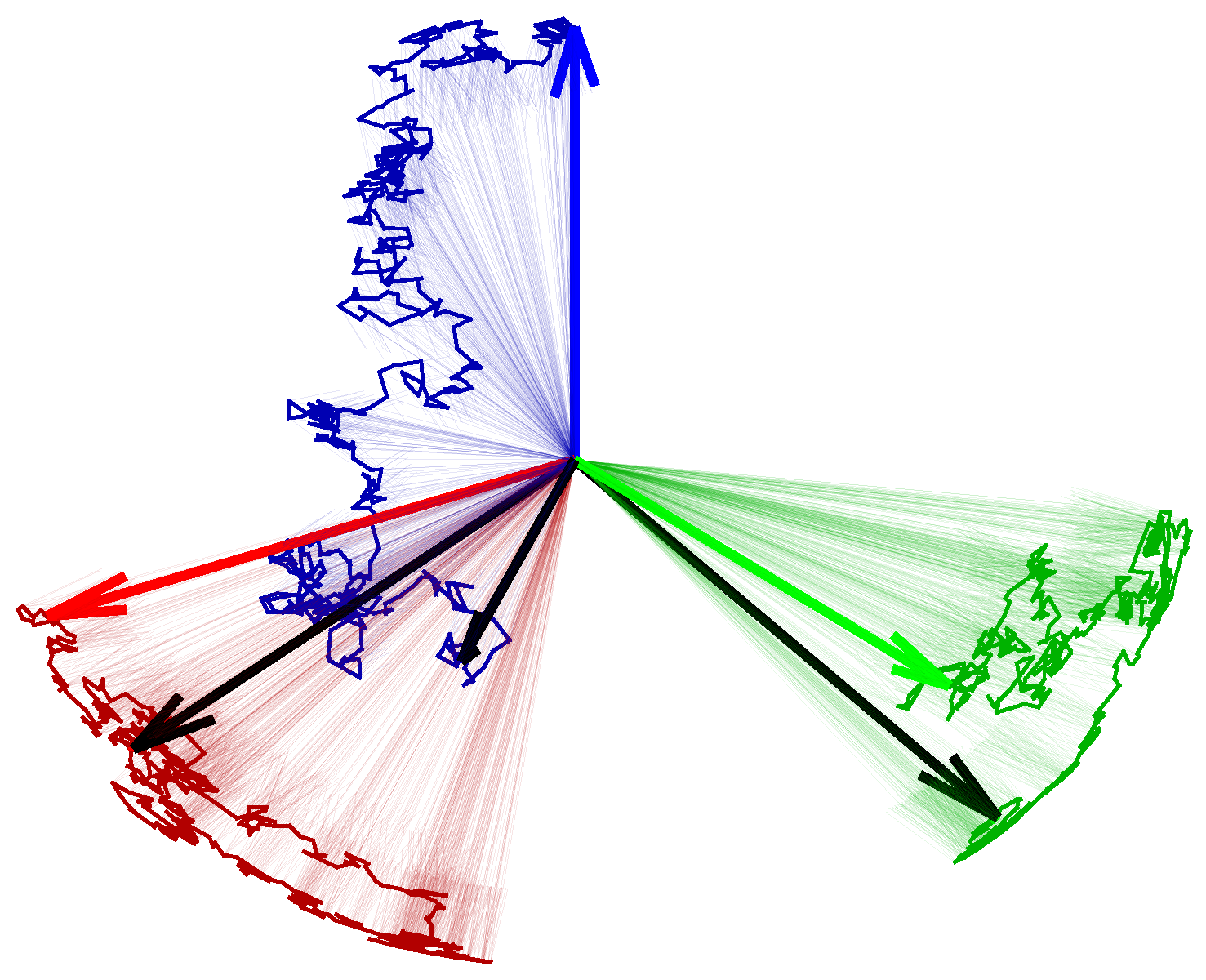
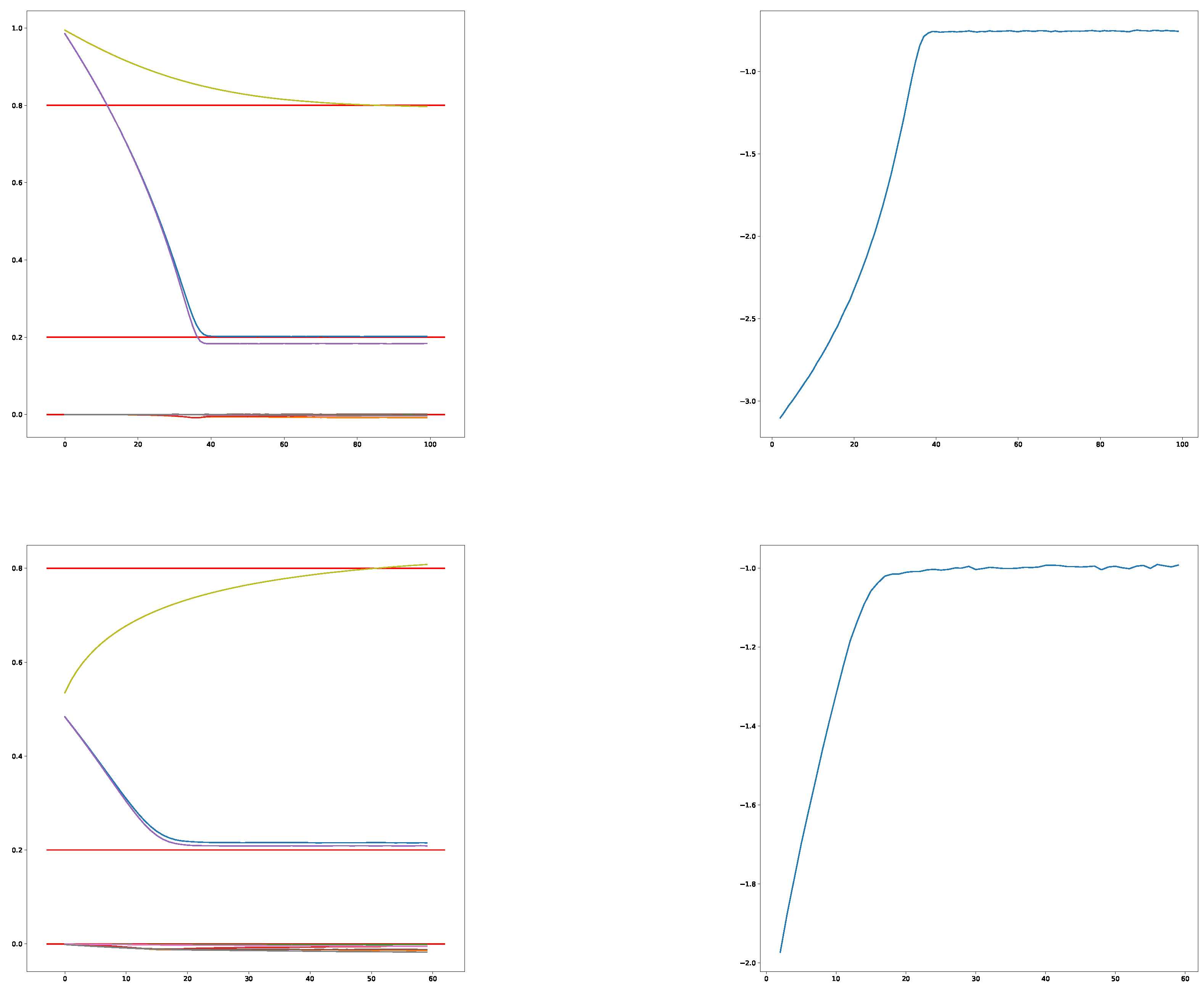
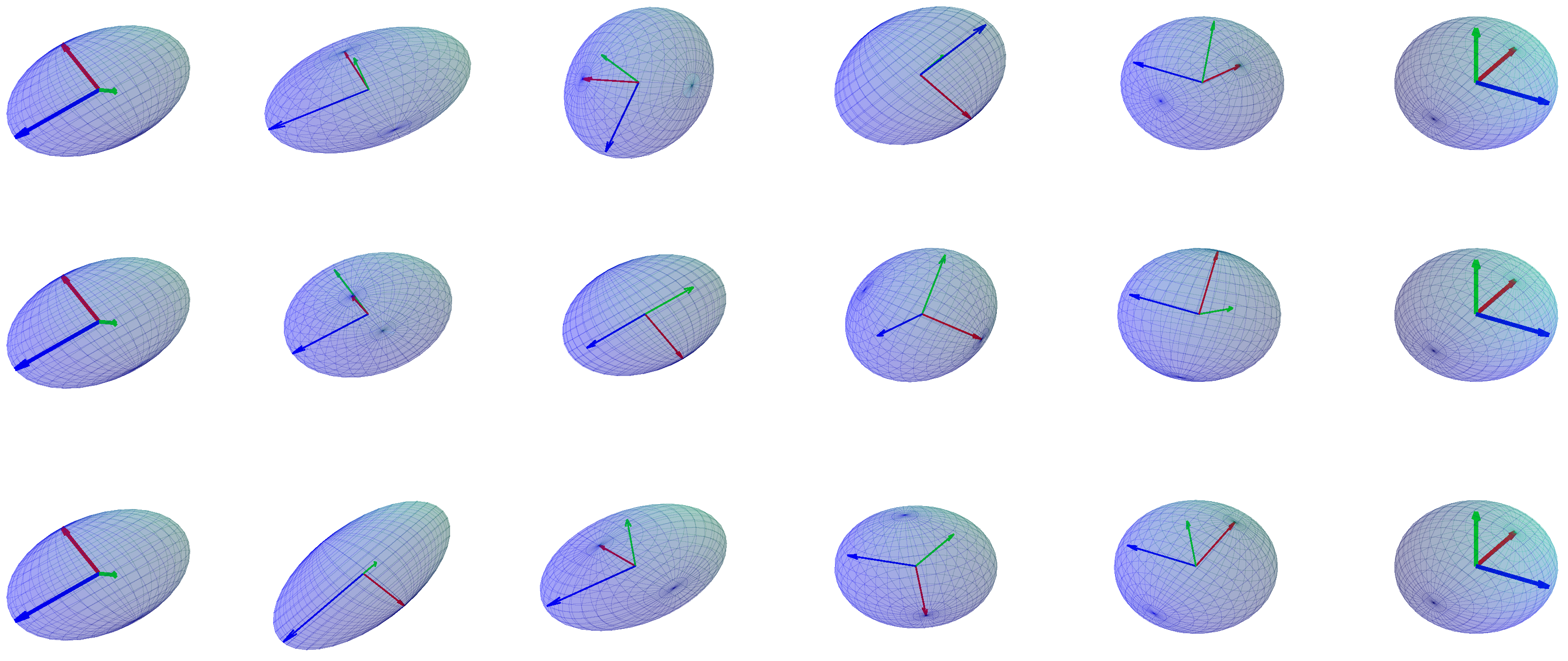
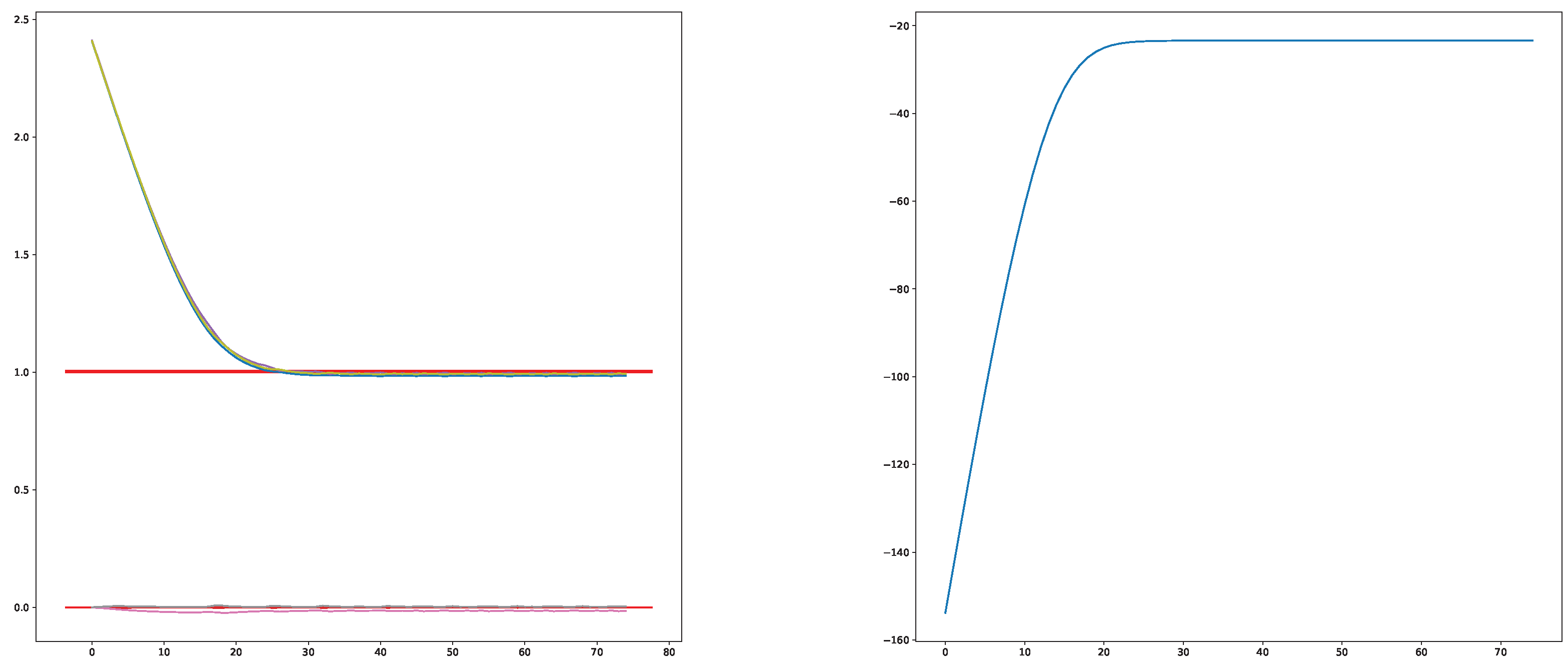
6.2. Importance Sampling and Metric Estimation on SO(3)

This section takes G as the special orthogonal group $\mathrm{SO}\left(3\right)$, the space of three-dimensional rotation matrices. The special orthogonal group is a compact connected matrix Lie group. The rotation group $\mathrm{SO}\left(3\right)$ is a semi-simple Lie group, and bi-invariant inner products exist. In the case of a bi-invariant metric, the Riemannian exponential map Exp coincides with the Lie group exponential map exp, and thus, the Riemannian distance function $d{(R,I)}^2={\parallel {Log}_I\left(R\right)\parallel }^2$, from the rotation R to the identity I, satisfies ${\nabla }_{R}d{(R,I)}^2=2log\left(R\right)$.

Figure 2 illustrates the numerical approximation with a sample path from the guided diffusion conditioned to hit the rotation represented by the black vectors. Another way of visualizing the guided bridge on the rotation group $\mathrm{SO}\left(3\right)$ is through the angle–axis representation. Figure 3 represents a guided process on $\mathrm{SO}\left(3\right)$ by presenting the axis representation on ${\mathbb{S}}^2$ and its corresponding angle of rotation.

Figure 4 illustrates how importance sampling on $\mathrm{SO}\left(3\right)$ leads to a metric estimation of the underlying unknown metric, which generated the Brownian motion. We sampled 128 points as endpoints of a Brownian motion from the metric $\mathrm{diag}(0.2,0.2,0.8)$, and used 20 time steps to sample four bridges per observation. An iterative MLE method using gradient descent with a learning rate of $0.2$ and initial guesses of the metric $\mathrm{diag}(1,1,1)$ and $\mathrm{diag}(0.5,0.5,0.5)$ yielded convergence to the true metric.

Figure 4. The importance sampling technique applies to estimate the metric on the Lie group $\mathrm{SO}\left(3\right)$. Sampling a Brownian motion from an underlying unknown metric, we obtain convergence to the true underlying metric using an iterative MLE method. Here, we sampled four guided bridges per observation, providing a relatively smooth iterative likelihood. (Top left) Estimation of the unknown underlying metric using bridge sampling, starting from the metric $\mathrm{diag}(1,1,1)$. Here, the true metric is the diagonal matrix $\mathrm{diag}(0.2,0.2,0.8)$ represented by the red lines. The diagonal is represented by the colors diag (purple, blue, yellow). (Top right) The corresponding log-likelihood evolution through the iterations. (Bottom left) Estimation of the unknown underlying metric using bridge sampling, starting from the metric $\mathrm{diag}(0.5,0.5,0.5)$. (Bottom right) The corresponding iterative log-likelihood.

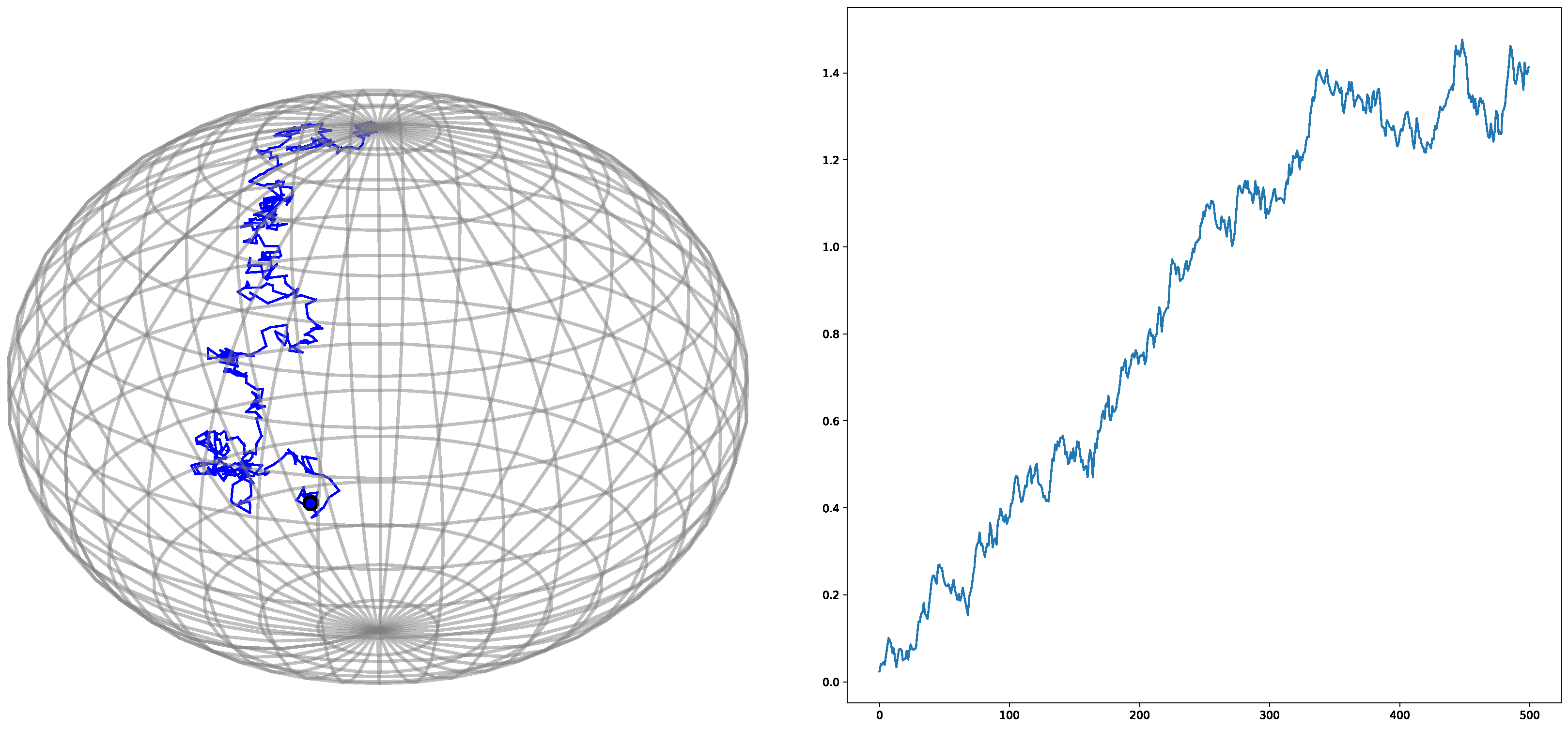
6.3. Diffusion Mean Estimation on the Space of Symmetric Positive Definite Matrices

The space of symmetric positive definite (SPD) matrices is used in a range of applications, one example being diffusion tensor imaging where the element of $SPD\left(3\right)$ models the anisotropic diffusion of water molecules in each position of the imaged domain. The SPD matrices constitute a homogeneous space ${\mathrm{GL}}_{+}\left(n\right)/\mathrm{SO}\left(n\right)$ of invertible matrices with the positive determinants’ quotient the rotation group.

Figure 5 illustrates discrete-time observations of three sample paths of a guided bridge in $SPD\left(3\right)$.

Figure 5. Discrete-time observations from three sample paths on $SPD\left(3\right)$. The sample paths are obtained as the pushforward of the Fermi bridge in ${\mathrm{GL}}_{+}\left(3\right)$. The start and endpoint are the left- and rightmost figures, where the SPD matrices are indicated by the bold face arrows.

In Figure 6, the bridge sampling scheme derived above is used to obtain an estimate of the diffusion mean [31,32] on $SPD\left(3\right)$ by sampling guided bridge processes in the space of invertible matrices with positive determinants ${\mathrm{GL}}_{+}\left(3\right)$. This sampling method provides an estimate of the density on ${\mathrm{GL}}_{+}\left(3\right)$, which projects to a density in $SPD\left(3\right)$. Exploiting the resulting density in $SPD\left(3\right)$, the iterative MLE yields convergence to the diffusion mean.

Figure 6. Given 256 data points in $SPD\left(3\right)$, we estimated the diffusion mean on the homogeneous space by sampling bridges in the top space conditioned on the fibers. The iterative MLE in Algorithm 1 yielded the convergence of the diffusion mean parameter, using a learning rate of $0.005$ and one bridge sample per observation. (Left) The purple, blue, and yellow lines correspond to the diagonal of the metric matrix, whereas the remaining colors represent the off-diagonal. The true mean value is the identity matrix indicated by the red lines. (Right) The corresponding log-likelihood evolution through the iterations.

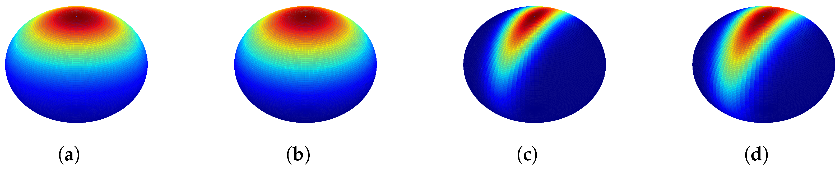
6.4. Density Estimation on the Two-Sphere

The two-sphere ${\mathbb{S}}^2$ can be considered the homogeneous space $\mathrm{SO}\left(3\right)/\mathrm{SO}\left(2\right)$ of three-dimensional rotations, identifying the subgroup of two-dimensional rotations as a single point. Conditioning on the fiber $\mathrm{SO}\left(2\right)$ in $\mathrm{SO}\left(3\right)$, we obtain guided bridges on ${\mathbb{S}}^2$. In the case of a bi-invariant metric on G, the G-valued Brownian motion pushes forward to an M-valued Brownian motion. Figure 1b illustrates the estimated transition density on ${\mathbb{S}}^2$ from sampling bridges in the Lie group conditioned on the fiber $\mathrm{SO}\left(2\right)$, when the underlying metric is bi-invariant. When altering the metric to a non-invariant variant one, the G-Brownian motion does not in general push forward to an M-Brownian motion. The non-invariant metrics result in a covariance structure exhibiting anisotropy, which is illustrated by Figure 1c,d.

7. Conclusions

In this paper, we presented algorithms for estimating the parameters of a class of densities that are the generalization of the Euclidean normal density to Lie groups and homogeneous spaces. We used the heat equation to generalize the normal distribution to Lie groups and homogeneous spaces, where the left- (or right-) invariant metric generalizes the notion of the covariance of a normal density. We presented algorithms for bridge simulation and for estimating the metric given the i.i.d. Lie group or homogeneous space-valued samples. The estimation algorithm was based on Monte Carlo simulations of Brownian bridges. These algorithms are expected to impact many diverse fields, including bioinformatics, medical imaging, shape analysis, computer vision, and information geometry, where Lie groups or homogeneous spaces are the natural model spaces for data samples.

8. Code

The code used for the experiments is available in the Theano Geometry http://bitbucket.org/stefansommer/theanogeometry and Jax Geometry http://bitbucket.org/stefansommer/jaxgeometry software packages (accessed on 7 July 2022). The implementation uses automatic differentiation libraries extensively for the geometry computations, as is further described in [33].

References

- Pedersen, A.R. Consistency and asymptotic normality of an approximate maximum likelihood estimator for discretely observed diffusion processes. Bernoulli 1995, 1, 257–279. [Google Scholar] [CrossRef]
- Bladt, M.; Sørensen, M. Simple simulation of diffusion bridges with application to likelihood inference for diffusions. Bernoulli 2014, 20, 645–675. [Google Scholar] [CrossRef]
- Bladt, M.; Finch, S.; Sørensen, M. Simulation of multivariate diffusion bridges. J. R. Stat. Soc. Ser. B Stat. Methodol. 2016, 78, 343–369. [Google Scholar] [CrossRef]
- Bui, M.N.; Pokern, Y.; Dellaportas, P. Inference for partially observed Riemannian Ornstein–Uhlenbeck diffusions of covariance matrices. arXiv 2021, arXiv:2104.03193. [Google Scholar]
- Delyon, B.; Hu, Y. Simulation of Conditioned Diffusion and Application to Parameter Estimation. Stoch. Process. Their Appl. 2006, 116, 1660–1675. [Google Scholar] [CrossRef]
- Jensen, M.H.; Mallasto, A.; Sommer, S. Simulation of Conditioned Diffusions on the Flat Torus. In Proceedings of the International Conference on Geometric Science of Information, Toulouse, France, 27–29 August 2019; Springer: Berlin/Heidelberg, Germany, 2019; pp. 685–694. [Google Scholar]
- Jensen, M.H.; Sommer, S. Simulation of Conditioned Semimartingales on Riemannian Manifolds. arXiv 2021, arXiv:2105.13190. [Google Scholar]
- Van der Meulen, F.; Schauer, M. Bayesian estimation of discretely observed multi-dimensional diffusion processes using guided proposals. Electron. J. Stat. 2017, 11, 2358–2396. [Google Scholar] [CrossRef]
- Papaspiliopoulos, O.; Roberts, G. Importance sampling techniques for estimation of diffusion models. Stat. Methods Stoch. Differ. Equ. 2012, 311–340. [Google Scholar]
- Schauer, M.; Van Der Meulen, F.; Van Zanten, H. Guided proposals for simulating multi-dimensional diffusion bridges. Bernoulli 2017, 23, 2917–2950. [Google Scholar] [CrossRef]
- Sommer, S.; Arnaudon, A.; Kuhnel, L.; Joshi, S. Bridge Simulation and Metric Estimation on Landmark Manifolds. In Proceedings of the Graphs in Biomedical Image Analysis, Computational Anatomy and Imaging Genetics, Lecture Notes in Computer Science, Quebec, QC, Canada, 10–14 September 2017; Springer: Berlin/Heidelberg, Germany, 2017; pp. 79–91. [Google Scholar]
- Bui, M.N. Inference on Riemannian Manifolds: Regression and Stochastic Differential Equations. Ph.D. Thesis, UCL (University College London), London, UK, 2022. [Google Scholar]
- Fisher, R. Dispersion on a Sphere. Proc. R. Soc. Lond. A Math. Phys. Eng. Sci. 1953, 217, 295–305. [Google Scholar] [CrossRef]
- Kent, J.T. The Fisher-Bingham Distribution on the Sphere. J. R. Stat. Soc. Ser. B (Methodol.) 1982, 44, 71–80. [Google Scholar] [CrossRef]
- Thompson, J. Brownian bridges to submanifolds. Potential Anal. 2018, 49, 555–581. [Google Scholar] [CrossRef]
- García-Portugués, E.; Sørensen, M.; Mardia, K.V.; Hamelryck, T. Langevin Diffusions on the Torus: Estimation and Applications. Stat. Comput. 2017, 29, 1–22. [Google Scholar] [CrossRef]
- Hamelryck, T.; Kent, J.T.; Krogh, A. Sampling Realistic Protein Conformations Using Local Structural Bias. PLoS Comput. Biol. 2006, 2, e131. [Google Scholar] [CrossRef] [PubMed]
- Pennec, X.; Fillard, P.; Ayache, N. A Riemannian Framework for Tensor Computing. Int. J. Comput. Vis. 2006, 66, 41–66. [Google Scholar] [CrossRef]
- Vaillant, M.; Miller, M.; Younes, L.; Trouvé, A. Statistics on Diffeomorphisms via Tangent Space Representations. NeuroImage 2004, 23, S161–S169. [Google Scholar] [CrossRef]
- Yang, L. Means of Probability Measures in Riemannian Manifolds and Applications to Radar Target Detection. Ph.D. Thesis, Poitiers University, Poitiers, France, 2011. [Google Scholar]
- Grenander, U. Probabilities on Algebraic Structures; Wiley: New York, NY, USA/London, UK, 1963. [Google Scholar]
- Jensen, M.H.; Joshi, S.; Sommer, S. Bridge Simulation and Metric Estimation on Lie Groups. In Proceedings of the Geometric Science of Information; Lecture Notes in Computer Science; Nielsen, F., Barbaresco, F., Eds.; Springer International Publishing: Cham, Switzerland, 2021; pp. 430–438. [Google Scholar] [CrossRef]
- Pennec, X.; Sommer, S.; Fletcher, T. Riemannian Geometric Statistics in Medical Image Analysis; Elsevier: Amsterdam, The Netherlands, 2020. [Google Scholar]
- Liao, M. Lévy Processes in Lie Groups; Cambridge University Press: Cambridge, UK, 2004; Volume 162. [Google Scholar]
- Shigekawa, I. Transformations of the Brownian motion on a Riemannian symmetric space. In Zeitschrift für Wahrscheinlichkeitstheorie und Verwandte Gebiete; 1984; pp. 493–522. [Google Scholar]
- Kendall, W.S. The radial part of Brownian motion on a manifold: A semimartingale property. Ann. Probab. 1987, 15, 1491–1500. [Google Scholar] [CrossRef]
- Barden, D.; Le, H. Some consequences of the nature of the distance function on the cut locus in a Riemannian manifold. J. LMS 1997, 56, 369–383. [Google Scholar] [CrossRef]
- Le, H.; Barden, D. Itô correction terms for the radial parts of semimartingales on manifolds. Probab. Theory Relat. Fields 1995, 101, 133–146. [Google Scholar] [CrossRef]
- Hsu, E.P. Stochastic Analysis on Manifolds; AMS: Providence, RI, USA, 2002; Volume 38. [Google Scholar]
- Thompson, J. Submanifold Bridge Processes. Ph.D. Thesis, University of Warwick, Coventry, UK, 2015. [Google Scholar]
- Hansen, P.; Eltzner, B.; Huckemann, S.F.; Sommer, S. Diffusion Means in Geometric Spaces. arXiv 2021, arXiv:2105.12061. [Google Scholar]
- Hansen, P.; Eltzner, B.; Sommer, S. Diffusion Means and Heat Kernel on Manifolds. arXiv 2021, arXiv:2103.00588. [Google Scholar]
- Kühnel, L.; Sommer, S.; Arnaudon, A. Differential Geometry and Stochastic Dynamics with Deep Learning Numerics. Appl. Math. Comput. 2019, 356, 411–437. [Google Scholar] [CrossRef]
Publisher’s Note: MDPI stays neutral with regard to jurisdictional claims in published maps and institutional affiliations. |
© 2022 by the authors. Licensee MDPI, Basel, Switzerland. This article is an open access article distributed under the terms and conditions of the Creative Commons Attribution (CC BY) license (https://creativecommons.org/licenses/by/4.0/).