High-Fidelity Surrogate Based Multi-Objective Optimization Algorithm

Abstract

The employment of conventional optimization procedures that must be repeatedly invoked during the optimization process in real-world engineering applications is hindered despite significant gains in computing power by computationally expensive models. As a result, surrogate models that require far less time and resources to analyze are used in place of these time-consuming analyses. In multi-objective optimization (MOO) problems involving pricey analysis and simulation techniques such as multi-physics modeling and simulation, finite element analysis (FEA), and computational fluid dynamics (CFD), surrogate models are found to be a promising endeavor, particularly for the optimization of complex engineering design problems involving black box functions. In order to reduce the expense of fitness function evaluations and locate the Pareto frontier for MOO problems, the automated multiobjective surrogate based Pareto finder MOO algorithm (AMSP) is proposed. Utilizing data samples taken from the feasible design region, the algorithm creates three surrogate models. The algorithm repeats the process of sampling and updating the Pareto set, by assigning weighting factors to those surrogates in accordance with the values of the root mean squared error, until a Pareto frontier is discovered. AMSP was successfully employed to identify the Pareto set and the Pareto border. Utilizing multi-objective benchmark test functions and engineering design examples such airfoil shape geometry of wind turbine, the unique approach was put to the test. The cost of computing the Pareto optima for test functions and real engineering design problem is reduced, and promising results were obtained.

1. Introduction

Numerous competing objectives and constraint functions, as well as time-consuming and expensive simulations, are present in the majority of real-world optimization issues. High-fidelity models must frequently be expensively modelled in order to address these problems. Finding the Pareto optimum of multi-objective optimization problems (MOO) necessitates evaluating expensive fitness and constraint functions. However, only a few tests are allowed in practice due to the restricted computing resources available to address such problems, notably black box functions. Researchers [1,2,3] found that the development of surrogate models employing a few high-fidelity solution assessments to replace computationally expensive models is promising and fruitful. Expensive functions are commonly replaced by surrogate models such as the radial basis function, Kriging, or response surface method [4].

In MOO problems demanding expensive computational analysis and simulation tools, for example FEA and CFD, surrogate models have grown in prominence and received more attention. Due to their capacity to imitate the real expensive model and their compliance with challenging computational requirements, surrogate models have been proved to be viable tools for MOO problems [5]. Numerous optimization applications demand labor- and resource-intensive fitness evaluations. The load considerably increases when dealing with multiple-objective black box functions that need to be evaluated. The automated MOO algorithm (AMSP) proposed in this paper is based on surrogate approximations.

The suggested algorithm automatically constructs an ensemble of surrogates from the three available surrogate models based on a methodology that will be introduced and explained in detail in this paper. The algorithm adaptively adjusts the effective surrogate model to determine the Pareto frontier for the MOO problem. The Response Surface Function (RSF), Radial Basis Function (RBF), and Kriging model are employed as surrogate approximations in this work [6,7,8,9,10,11]. To fully make use of the potential design space, an efficient sampling technique must be used. Traditional sampling techniques are afflicted by the “curse of dimensionality”, which causes an exponential increase in the number of sampling points needed to explore the design space as the number of design variables rises. The Latin Hypercube Designs (LHD) method [12] was consequently modified in this work. LHD is renowned for randomly and evenly covering the practicable portion of the design space in its sampling. These significantly reduce computation costs and increase the probability of finding the Pareto frontier for MOO problems. The suggested algorithm (AMSP) consistently and accurately locates the Pareto frontier for MOO problems. The computational cost is significantly reduced when AMSP is used to locate the Pareto frontier for expensive black-box functions. AMSP was put to the test using benchmark test problems and actual, realistic engineering challenges in order to show off its performance. The outcomes are seen as promising and encouraging.

2. Literature Review

MOO has emerged as a possible approach to overcoming obstacles with conflicting goals. The most effective trade-offs between a set of criteria are often determined by using a group of Pareto optima to solve MOO issues. Finding the final Pareto frontier for use in practice is challenging, especially when there are several competing objectives to take into account.

In situations with two or three objective functions, it may be rather simple to describe the set of Pareto-optimal solutions in the objective function space. When we identify Pareto limits, we may completely understand the relationship between trade-offs between objectives. It has been demonstrated that surrogate models may accurately and efficiently identify Pareto-optimal solutions.

Effective and durable search strategies are greatly needed to tackle such challenging multi-objective optimization problems. The majority of algorithms are evolutionary ones such as GA, PSO, and others. Black box functions have only been shown for a select few. These are the solutions provided for multi-objective optimization problems that demand pricey analysis and simulation methods, such as multi-physics modeling and simulation, FEA, and CFD analyses. The optimization of computationally expensive black box functions needs more focus and should be addressed due to the challenges these functions have presented to the optimization community. A promising method that might help with the resolution of these problems is the use of surrogate models. The expensive model (function) is simulated and predicted using surrogate models, which have a reduced computational cost. MOOP with expensive high fidelity computational models, such as sophisticated simulations and thorough analyses, the standard multi-objective optimization methods, are challenging to perform directly due to the high computational cost of objective and constraint function evaluations. As a response to these problems, surrogate models gain in popularity.

There are typically two scenarios in which black box functions are used to address MOO problems. Numerous evolutionary algorithms (EAs) use the first scenario, which closely resembles the Pareto optimal [13,14,15]. Due to the costly evaluations of numerous non-Pareto set points required by these approaches, they are renowned for being computationally expensive. In the second scenario, surrogate models are used to assess each objective function. Naturally, the constructed surrogate models will determine how precise the Pareto-optimal border is.

Li et al. [16] created a hyper-ellipse surrogate to approach the Pareto optimum frontier for bicriteria convex optimization problems. If the established approximation model is not sufficiently accurate, the Pareto-optimal frontier will not be considered a good approximation of the genuine Pareto-optimal frontier. In order to make use of the multi-objective design region and find the Pareto set using approximation models, Wilson et al. [17] used two surrogate approximations (response surface and Kriging models). Prior to applying the optimization strategy, they employ a technique that minimizes the loss of surrogate approximation accuracy. Proos et al. [17] used the weighted and global criterion technique to construct an algorithm that incorporates several criterion optimizations into evolutionary structural optimization (ESO). Yang et al. [15] developed a strategy for managing surrogate models for MOO. The framework includes a sequentially-updated surrogate model and a GA-based method. Instead of before, as in the preceding case, the surrogate model is altered during the optimization process [14]. The accuracy of the surrogate model is crucial for maintaining the integrity of the identified border sets in their proposed method.

Yang’s [15] research had a hard time locating frontier areas close to the extremes. The Pareto Set Pursuing (PSP) technique, proposed by Shan and Wang [18], entails creating sampling guidance functions based on surrogate models. It was said that PSP had enormous promise in terms of effectiveness, accuracy, and robustness. An artificial neural network (ANN) approximation was merged with NSGA-II by Nain and Deb [19] in order to achieve a computationally efficient search and enable the use of GAs on computationally expensive problems. A progressively updated design and analysis of computer experiments (DACE) model-based extended efficient global optimization method (ParEGO) for MOO challenges is presented by Knowles [20]. In order to develop a multi-objective design optimization approach, Kim and Chung [21] combined GA with Kriging. The developed method was tested in a wing platform design competition, proving its efficacy and viability. A novel multi-objective optimization approach based on the usage of surrogate models was developed by Liu et al. [22]. In each iteration, the approximation models are gradually produced by the response surface approximations. The Pareto optimum set proposed by the approximations is located using a multi-objective genetic algorithm. The proposed approach relies less on the accuracy of the surrogate models because it concentrates on identifying the real Pareto ideal. Lim in [23] explored the use of substitute models in evolutionary search. Jang in [24] employed an adaptive approximation framework to address the processing cost of the entire stochastic fatigue analysis in the optimization process.

An adaptive Kriging model was created by Yang et al. [25] that increases the accuracy of the approximations by adding additional points to the model with each iteration. Zhao et al. [26] suggested a dynamic Kriging methodology, which uses several sets of approximation functions in various groups of points, was proposed as a way to regulate the nonlinearity of the model space [26]. The suggested technique has proven to be extremely successful when applied to challenging optimization problems [27]. By automatically choosing pertinent surrogates during the search process, Gu et al. [28] developed an optimization approach to increase search efficiency by integrating a dynamic Radial Basic Function (RBF) with an adaptive sampling technique. Diez et al. [29] developed a method for improving both the existing solution and the approximation model. A dynamic RBF function-based strategy was developed by Volpi et al. [30] who claimed it was successful in solving high-dimensional problems. Iuliano [31] examined and discussed a number of adaptation strategies.

The proposed algorithm is designed to handle highly non-linear black-box multi-objective optimization problems. The algorithm is unique because it takes advantage of three surrogates to identify the Pareto set and the Pareto frontier with less computational cost. AMSP adaptively combines three surrogate models based on a selection criterion that will be discussed later. To find the Pareto frontier for the multi-objective problem, the method automatically assigns a weight factor to each surrogate model based on calculated RMSE values. LHD was utilized to generate sampling points to refine the search for optimal Pareto sets. AMSP uses the ensemble of surrogates to identify the Pareto frontier. These factors aided in the decrease of computation costs and boosted the likelihood of identifying the Pareto frontier for MOO problems.

3. Multi-Objective Optimization

MOO is defined as a set of design variables that satisfy constraints and optimize a vector function whose constituents are the objective functions. It can be expressed as follows:

Optimize the vector function

$$\overline{f}\left(\overline{x}\right)={\left[f_1\left(\overline{x}\right),f_2\left(\overline{x}\right),\dots ,f_k\left(\overline{x}\right)\right]}^T$$

(1)

by determining the decision variables vector;

$${\overline{x}}^{*}={\left[x_1^{*},x_2^{*}, \dots ,x_n^{*} \right]}^T$$

(2)

which will satisfy the m inequality constraints

$$g_i\left(\overline{x}\right)\ge 0, i=1,2,\dots ,m$$

(3)

and the p equality constraints

$$h_j\left(\overline{x}\right)=0, j=1,2,\dots ,p$$

(4)

where $x={\left[x_1,x_2,\dots x_n\right]}^T$ is the vector of decision variables. In other words, we wish to determine from among the set $f$ of all numbers, which satisfy Equations (3) and (4). In particular set $x_1^{*},x_2^{*}\dots x_k^{*}$ which yields the optimum values of all the objective functions.

Pareto Frontier

The Pareto frontier or Pareto set is the set of all Pareto-efficient results. If no feasible vector $x$ exists that decreases some objective functions while simultaneously increasing at least one other objective function, then the vector of, $x^{*}$ is Pareto-optimal. Following are some mathematical ways to express the Pareto optimality:

A vector of $x^{*}$ is a Pareto optimum if and only if, for any $x$ and i,

$$f_j\left(x\right)\le f_j\left(x^{*}\right), j=1,\dots ,m; j\ne i, f_i\left(x\right)\ge f_i\left(x^{*}\right)$$

(5)

Finding Pareto set points allows for the discovery of a Pareto frontier, which is the main purpose of multi-objective optimization (MOO). Claiming that these points are in the Pareto set or the Pareto frontier is challenging unless there is a strong method to determine whether they are in the set or not. This could be quickly ascertained if a fitness function is customized. The fitness function, which was utilized in this paper, will be discussed in the section that follows.

4. The Proposed Algorithm

The proposed algorithm’s main objective is to identify the Pareto frontier with the least amount of computing time for expensive black-box functions. This goal can be achieved if appropriate tools, such as effective sampling techniques, are used. Because it provides equal and random samples in the design space, the LHD sampling technique is used in this work. The Pareto frontier should be approached repeatedly whenever more samples are generated. A sampling guidance function is needed to judge if these sample sites are near to or on the Pareto frontier. The following section introduces the sampling guidance procedure.

4.1. Sampling Procedure

There are many statistical methods available today for creating sample points based on a specific probability density function (PDF). Latin Hypercube Designs (LHD) sampling technique was used to create random and evenly distributed sample points in the design space of interest. The search process starts with the creation of a surrogate approximation model from a small number of sample points, then generates many points using the model. Finally, the points are sorted, and a cumulative function that is similar to the cumulative density function (CDF) proposed in [32] is created by adding up all the function values. The generation of sample points based on a specific probability density function can be done statistically using a variety of methods nowadays (PDF). Latin Hypercube Designs (LHD) sampling technique was used to create random and evenly distributed sample points in the design space of interest. The search starts by building a surrogate model from a small number of sample points, then generates many points using the surrogate model, sorts the points, and then builds a cumulative function similar to the cumulative density function (CDF) proposed in [32] by adding up all the function values.

4.2. Surrogate Models

In this study, surrogate models served as crucial research tools. Three popular surrogate approximations were used: Kriging, RBF, and RSM. The next sections present each surrogate along with its mathematical formulations.

4.2.1. Kriging

The Kriging model is one of the most well known spatial interpolation models for substituting the numerical relationship between input and output variables. It loses a lot of efficiency when dealing with significant design variances. On the other hand, Kriging surrogate models can significantly reduce the computational cost of regression because they need significantly fewer sample data to be generated. Additionally, more trustworthy prediction results can be produced because the Kriging fitting technique concentrates on more representative samples.

The Kriging model regards the function of interest as a realized random function (stochastic process). As a result, a linear combination of a global model and deviations, Equation (6), is presented as the Kriging mathematical model:

$$y\left(x\right)=f\left(x\right)+Z\left(x\right)$$

(6)

where $y\left(x\right)$ is the unknown deterministic response, $f\left(x\right)$ is a known (usually polynomial) function of x, and $Z\left(x\right)$ is a realization of a stochastic process with mean zero, variance ${\sigma }^2$, and non-zero covariance.

4.2.2. Radial Basis Function (RBF)

The interpolation of scatter data using radial basis functions has been shown to be highly accurate in high-dimensional problems. Radial basis function interpolation, Equation (7), is used to approximate the form.

$$\widehat{f}\left(x\right)=\sum _{n=1}^N{\omega }_n\phi \left(x-x_n\right)$$

(7)

where $\phi \left(x\right)$=$\varnothing (\Vert x\Vert )$ is a radial function. The positions $x_n, n=1\dots N$ are known as the RBF centers.

4.2.3. Response Surface Function (RSF)

RSF was initially created to model experimental results [6], after which it was expanded to include numerical experiment modeling. RSF is used in design optimization to reduce the cost of pricey analytical methods (for example, FEA or CFD analyses) as well as the related numerical noise. Equation (8) can be used to express the response function:

$$y=f\left(x_1,\dots ,x_n\right)+\epsilon$$

(8)

where $\epsilon$ represents the noise or the error observed in the response $y$. The surface represented by $f\left(x_1,\dots ,x_n\right)$ is called a response surface.

4.3. Ensemble of Surrogate Models

The three surrogate models, RSF, RBF, and KRG, are integrated in an appropriate linear approach to produce a better-weighted ensemble of surrogates that can duplicate the high-fidelity surrogate in the feasible region of the design space.

Equation (9) represents the ensemble of surrogate’s equation:

$${\widehat{y}}_{ensemble}\left(x\right)={\beta }_{q}RSF\left(x\right)+{\beta }_{r}RBF\left(x\right)+{\beta }_{k}KRG\left(x\right)$$

(9)

where

$${\beta }_q+{\beta }_r+{\beta }_k=1$$

(10)

where ${\widehat{y}}_{ensemble}\left(x\right)$ is the surrogate model to the analysis/simulation function, $f\left(X\right)$, at sample point x; $RSF\left(x\right),RBF\left(x\right) \mathrm{and} KRG\left(x\right)$ represents the RSF, RBF and KRG surrogate models respectively; ${\beta }_q,{\beta }_r\mathrm{and}{\beta }_k$ are weighted coefficients that control how much each model contributes to the combined surrogate.

4.4. Automated Ensemble of Surrogate’s Selection

Three surrogate models are built after producing a few sample points in the space of interest using Latin Hypercube Designs. RSF, RBF and Kriging. These surrogates’ root mean square error (RMSE) is calculated. In the next step, the surrogate with the highest RMSE value (close to 1) is chosen to be heavily depended on and assigned high weight factor and the one with low RMSE (close to zero) is assigned the lowest weight factor. Kriging typically yields lower RMSE than RSF and RBF. In this method, a rule was established to guide the mixed surrogate construction process, which is to first assess the RMSE and then automatically assign weight factor based on the value of the RMSE. The weight factor is selected as percentage so that the surrogate with RMSE close to 1 gets a weight factor 60% and the one with low RMSE gets a weight factor of 10%. The surrogate that yields RMSE in between gets 30% weight factor. If RMSE is close to 1, build Kriging. If the contrary is true, then build either RSF or RBF based on which one has RMSE closer to 1.

4.5. Maximum Fitness Function

There are numerous approaches to define the fitness function for an objective function problem. The function that comes next is known as the maximal fitness function. Equation (11) identifies the fitness function used in this study. Numerous programs have successfully exploited this capability. Equation (12) illustrates the modified maximum fitness function that was used in this study.

$$P\left(x_i\right)=\underset{j\ne i;j\in P}{\underbrace{max}}{\displaystyle [}\underset{1\le s\le k}{\underbrace{min}}\left\{f_s\left(x_i\right)-f_s\left(x_j\right)\right\}{\displaystyle ]}$$

(11)

$$P_i=max\left(min\left(f_{s1}^i-f_{s1}^j, f_{s1}^i-f_{s1}^j,\dots ,f_{sm}^i-f_{sm}^j\right)\right)$$

(12)

where, $P_i$ denotes the fitness value of the ith design; $f_{sk}^i$ is scaled to kth objective function value of the ith design, $k=1,\dots ,m$. The max in Equation (12) is over all other designs j ≠ i in the set and the min is over all the objectives. The objectives $f_{s1}, f_{s2}, \dots , f_{sm}$ in Equation (13) are scaled to a range [0, 1]. For example, for $f_{s1}^i$,

$$f_{s1}^i=\frac{unsc{f}_{1,i}-unsc{f}_{1,min}}{unsc{f}_{1,max}-unsc{f}_{1,min}}$$

(13)

where, $unsc{f}_{1,i}$ denotes the un-scaled value of the first objective for the ith design; $unsc{f}_{1,min}$ denotes the maximum $f_{s1}^i$ un-scaled value of the first objective among all designs; and $unsc{f}_{1,min}$ denotes the minimum un-scaled value of the first objective among all designs. In case that an objective function is a constant, the scaled objective function value is taken as 1 in this work.

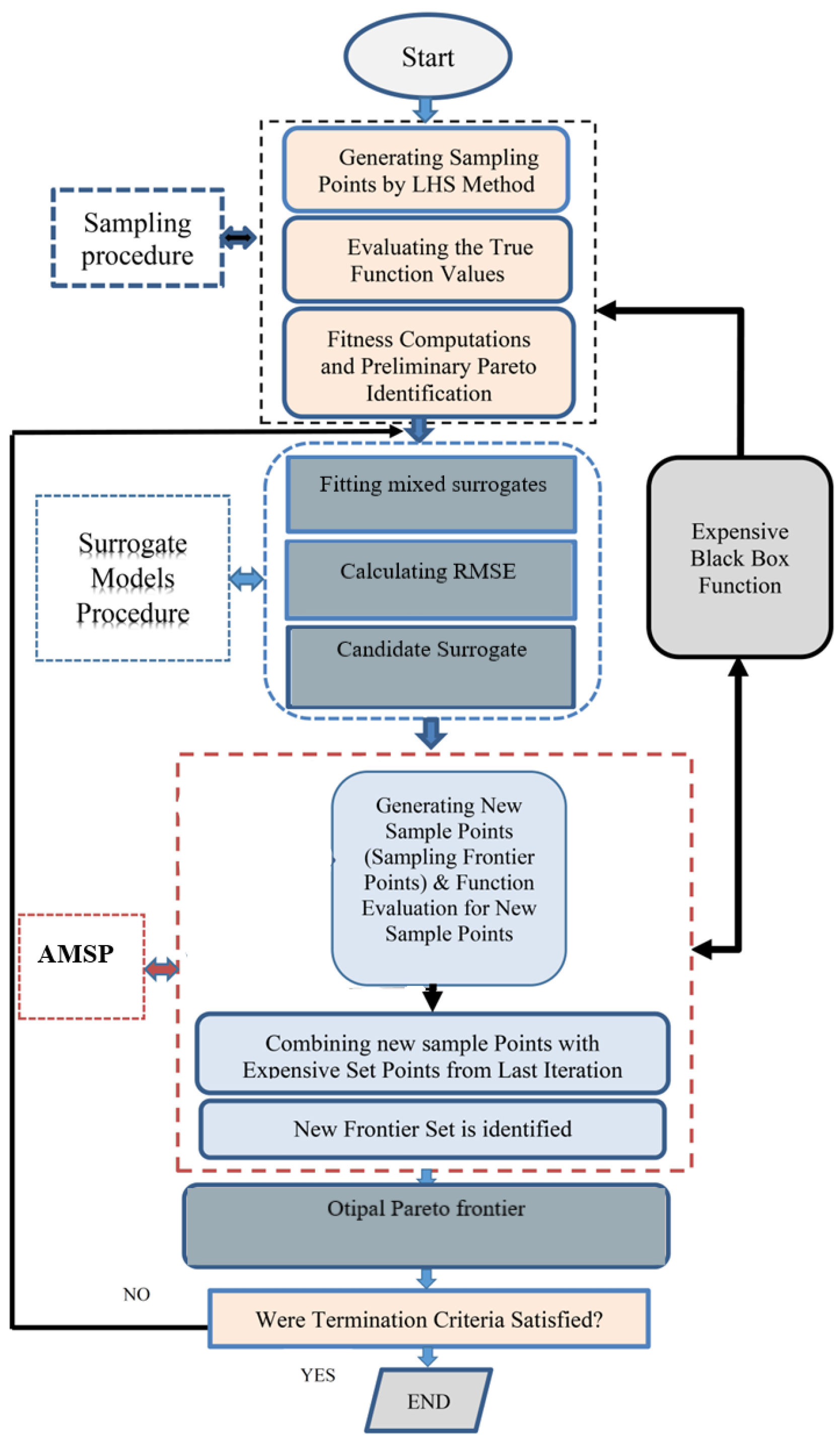
4.6. The Proposed Algorithms Steps:

The steps of the suggested approach are summarized and discussed in the steps below:

• Sampling initial random design points. Creating a small number of randomly distributed sample points in the design space. The sample procedure is carried out using LHD [12].
• The black box function (expensive function) is used to detect the current frontier points after evaluating the generated sample points.
• Calculating the built surrogates’ root mean square error (RMSE). In this step, three mixed surrogates are introduced to imitate and replace the expensive function: the response surface function (RSF), radial basis function (RBF), and Kriging (KRG) surrogate model. After these substitutes are fitted to the previously acquired sample points, RMSE is calculated. The surrogate with a higher RMSE value (near to 1) is automatically adjusted by the algorithm, and it is given a higher weight factor than the other surrogates with lower RMSE values (close to 0). The surrogate with the lowest RMSE values receives a weight percentage of 10%, the surrogate with the highest RMSE values receives a weight percentage of 60%, and the surrogate with all other RMSE values receives a weight percentage of 20%. The subsequent stages should make use of the selected mixed surrogate.
• Creating a lot of cheap points in a short amount of time. They are used to assess the enormous number of sample points produced by LHD after the development of the mixed surrogate (cheap function).
• Combining the sample points. The preliminary approximated Pareto border is identified or moved towards in this stage by combining all generated sample points (expensive and cheap locations).
• Identifying the candidate points out of all the ones that already exist (points obtained in the previous step). These points are very likely to become Pareto set points.
• For fresh sample points, evaluate fitness functions. The expensive black-box functions were used to evaluate the points collected in step 5.
• To identify the new frontier set, new sample points are combined with expensive frontier points.
• If convergence criteria (termination criteria) are met, the method ends; otherwise, return to step 4.

4.7. Termination Criterion

Two termination criteria were adapted in this work.

• If the difference between frontier points after two consecutive iterations is less than 0.0001, then terminate: and
• If the maximum number of specified number of iterations has been reached, then the algorithm should terminate.

Figure 1 depicts the proposed approach’s flow diagram. It explains how the algorithm works in a nutshell.

5. Numerical Examples and Results

The suggested approach is tested and validated using a number of well-known multi-objective optimization benchmark test functions from the literature, which are reported in Table 1. The results of the four test issues are shown in this section. The results of optimizing a real-world example are also provided in this section.

5.1. Test Functions

The test functions tested using the proposed approach are reported in Table 1.

Table 1. Multi-objective test functions.

	Test Function	Constraints	Domain
F1	$\mathrm{Minimize} f_1\left(x\right)={\left(x_1^2-5\right)}^2+{\left(10x_2/A-6\right)}^2;$$\mathrm{Minimize} f_2\left(x\right)={\left(x_1^2-7\right)}^2+{\left(10x_2/A-6\right)}^2$		x1, x2 ϵ [−10, 10] Where A = 10
F2	$\mathrm{Minimize} f_1\left(x\right)={\left(x_1\right)}^5+x_2;$ $\mathrm{Minimize} f_2\left(x\right)={\left(x_1\right)}^5+1-x_2$		$x_1,x_2$ ϵ [0, 1]
T1	$\mathrm{Minimize} f_1\left(x\right)={\left(x_1-2\right)}^2+{\left(x_1-1\right)}^2;$$\mathrm{Minimize} f_2\left(x\right)=x_1{}^2+{\left(x_2-6\right)}^2$	$h\_1\left(x\right)=x\_1-1.6\le 0;$ $h_2\left(x\right)=0.4-x_1\le 0$; $h_3\left(x\right)=x_2-5\le 0$; $h_2\left(x\right)=2-x_2\le 0$	$x_1$ ϵ [0.4, 1.6] $x_2$ ϵ [2, 5]
T2	$\mathrm{Minimize} f_1\left(x\right)={\left(x_1+x_2-7.5\right)}^2+{\left(x_2-x_1+31\right)}^2/4;$$\mathrm{Minimize} f_2\left(x\right)={\left(x_1-1\right)}^2/4+\left(x_2-4^2\right)/2$	$h\_1 \left(x\right)=2.5-\left(x\_1-2\right)^3⁄\left(2-x\_2\right)\le 0;$$h\_2 \left(x\right)=3.85+8\left(x\_2-x\_1+0.65\right)^2-x\_2-x\_1\le 0$	$x_1$ ϵ [0, 5] $x_2$ ϵ [0, 3]
T3	$\mathrm{Minimize} f_1\left(x\right)=25-\left(x_1^3+x_1^2\left(1+x_2+x_3\right)+x_2^3+x_3^3\right)/10;$$\mathrm{Minimize} f_2\left(x\right)=35-\left(x_1^3+2x_2^2+x_2^2\left(2+x_1+x_3\right)+x_3^3\right)/10;$$\mathrm{Minimize} f_3\left(x\right)=50-\left(x_1^3+x_2^3+3x_3^3+x_3^2\left(3+x_1+x_3\right)\right)/10;$	$h\_1 \left(x\right)=12-x\_1^2-x\_2^2-x\_3^2\ge 0$	$x_1,x_2,x_2$ ϵ [0, 5]

Table 1. Multi-objective test functions.

	Test Function	Constraints	Domain
F1	$\mathrm{Minimize} f_1\left(x\right)={\left(x_1^2-5\right)}^2+{\left(10x_2/A-6\right)}^2;$$\mathrm{Minimize} f_2\left(x\right)={\left(x_1^2-7\right)}^2+{\left(10x_2/A-6\right)}^2$		x1, x2 ϵ [−10, 10] Where A = 10
F2	$\mathrm{Minimize} f_1\left(x\right)={\left(x_1\right)}^5+x_2;$ $\mathrm{Minimize} f_2\left(x\right)={\left(x_1\right)}^5+1-x_2$		$x_1,x_2$ ϵ [0, 1]
T1	$\mathrm{Minimize} f_1\left(x\right)={\left(x_1-2\right)}^2+{\left(x_1-1\right)}^2;$$\mathrm{Minimize} f_2\left(x\right)=x_1{}^2+{\left(x_2-6\right)}^2$	$h\_1\left(x\right)=x\_1-1.6\le 0;$ $h_2\left(x\right)=0.4-x_1\le 0$; $h_3\left(x\right)=x_2-5\le 0$; $h_2\left(x\right)=2-x_2\le 0$	$x_1$ ϵ [0.4, 1.6] $x_2$ ϵ [2, 5]
T2	$\mathrm{Minimize} f_1\left(x\right)={\left(x_1+x_2-7.5\right)}^2+{\left(x_2-x_1+31\right)}^2/4;$$\mathrm{Minimize} f_2\left(x\right)={\left(x_1-1\right)}^2/4+\left(x_2-4^2\right)/2$	$h\_1 \left(x\right)=2.5-\left(x\_1-2\right)^3⁄\left(2-x\_2\right)\le 0;$$h\_2 \left(x\right)=3.85+8\left(x\_2-x\_1+0.65\right)^2-x\_2-x\_1\le 0$	$x_1$ ϵ [0, 5] $x_2$ ϵ [0, 3]
T3	$\mathrm{Minimize} f_1\left(x\right)=25-\left(x_1^3+x_1^2\left(1+x_2+x_3\right)+x_2^3+x_3^3\right)/10;$$\mathrm{Minimize} f_2\left(x\right)=35-\left(x_1^3+2x_2^2+x_2^2\left(2+x_1+x_3\right)+x_3^3\right)/10;$$\mathrm{Minimize} f_3\left(x\right)=50-\left(x_1^3+x_2^3+3x_3^3+x_3^2\left(3+x_1+x_3\right)\right)/10;$	$h\_1 \left(x\right)=12-x\_1^2-x\_2^2-x\_3^2\ge 0$	$x_1,x_2,x_2$ ϵ [0, 5]

5.2. Wind Turbine Airfoil Geometry Optimization

The geometry of a typical GT compressor blade airfoil [33] is optimized in this example using the suggested algorithm. In both design and off-design scenarios, the objective is to lower the total pressure loss coefficient. NURBS curves were used to parameterize the geometry input used in the optimization process. This method treats the positions of the non-uniform rational basis spline (NURBS) control points as design variables. Four NURBS curves for each of the four segments of the compressor airfoil, each having nine control points, make up the airfoil. Because each control point has two coordinates, x and y, there are a total of 72 design variables. The junction points of the segments are one of 16 known and set parameters. The remaining 16 parameters are found by enforcing C2-continuity (which requires the second derivative to be zero at the endpoints) at the intersections of the segments. As a result, 40 variables will remain as design variables in the optimization procedure. However, to limit the number of design factors while maintaining a high level of geometric flexibility, the geometry of the leading edge (LE) and trailing edge (TE) is maintained constant to save CPU time.

The results of the airfoil optimization procedure strongly depend on the formulation of the objective function. In order to simulate 2-D fluid flow, the geometry code creates parameterized profiles that are then imported into the computational fluid dynamics program COMSOL CFD. The acceptable profiles’ post-processed outputs are then fed into the fitness calculation portion, where the airfoil loss values, L, should be minimized with respect to any shape. The single objective function is shown in Figure 2 as follows:

$$\begin{gathered} Minimize L_1\%=\left(a_1{L}_s\right)\ast 100 \\ Minimize L_2\%=\left(a_2{L}_d\right)\ast 100 \\ Minimize L_3\%=\left(a_3{L}_c\right)\ast 100 \end{gathered}$$

(14)

Subject to:

$$\begin{gathered} \left(\left|y_3-y_7\right| and \left|y_3-y_8\right|\right)\ge \mathrm{15\%} \mathrm{of}\mathrm{the}chord \\ 0\le x_i/chord\le \mathrm{100\%} \\ \mathrm{40\%}\le y_i/chord\le \mathrm{55\%} \end{gathered}$$

(15)

where a_i are weighting factors. The reduction of total pressure loss on the right (L_c) and left (L_s) sides of the design point significantly expands the operating range. The quantities y_i and x_i are design variables as shown in Figure 2.

The following are the weighting factors for the optimization process: a₁ = 0.20, a₂ = 0.70, and a₃ = 0.10.

$$\begin{gathered} L_s={\left(P_{o1}-P_{o2}\right)}_{stall}/0.5\rho V_1^2, L_d={\left(P_{o1}-P_{o2}\right)}_{des}/0.5\rho V_1^2, \\ {L}_c={\left(P_{o1}-P_{o2}\right)}_{Choke}/0.5\rho V_1^2, \end{gathered}$$

(16)

where P_o1 is intake total pressure, P_o2 is outlet total pressure, and V₁ is inlet velocity.

6. Results and Discussion

Multiple benchmark multi-objective optimization problems and a real-world engineering design challenge were used to test the proposed technique. Promising outcomes were gathered using the suggested algorithm. There were numerous computational optimization runs (approximately five runs). As noted earlier,

Table 2. Test results of the introduced algorithm on multi-objective test functions.

F1						F2
Run	Ite.	Eval	#Par.P	Surr.	RMSE	Run	Ite.	Eval	Par.P	Suur.	RMSE
1	37	75	48	RBF	0.9901	1	24	246	137	RBF	0.9721
2	32	61	45	RSF	0.9899	2	22	281	188	KRG	0.9704
3	23	56	35	KRG	0.9879	3	23	275	167	RBF	0.9569
4	30	66	43	RBF	0.9744	4	21	458	309	RSF	0.9565
5	33	71	47	RSF	0.9904	5	20	410	357	RBF	0.9777
T1						T2
Run	Ite.	Eval	#Par.P	Surr.	RMSE	Run	Ite.	Eval	Par.P	Suur.	RMSE
1	19	446	363	RBF	0.9812	1	27	58	39	RSF	0.9744
2	19	443	358	RSF	0.9963	2	29	59	37	RBF	0.9730
3	16	368	306	KRG	0.9811	3	34	73	44	KRG	0.9773
4	17	379	313	RSF	0.9792	4	28	65	44	RSF	0.9302
5	15	332	264	RBF	0.9971	5	38	87	46	RBF	0.9565
T3						P1
Run	Ite.	Eval	#Par.P	Surr.	RMSE	Run	Ite.	Eval	Par. P	Suur.	RMSE
1	250	1216	760	RSF	0.9325	1	1172	18,857	3464	RSF	0.9772
2	234	1213	765	RBF	0.9355	2	1218	19,934	3615	RSF	0.9821
3	273	1294	793	RBF	0.9781	3	986	16,582	3146	RSF	0.9763
4	232	1170	752	RSF	0.9932	4	1019	19,121	3623	RBF	0.9775
5	219	1172	729	RBF	0.9946	5	997	18,587	3455	RBF	0.9801

# Par. P = Number of Pareto points.

presents samples of the outcomes from five separate runs. The actual, real-world example (geometry of the airfoil in a wind turbine) required between 986 and 1172 iterations, with 242 serving as the median. The median number of function evaluations is 1213, with a range of 16,582 to 19,934. RBF surrogate model is the winner in the majority of test runs. The median number of convergent Pareto points, which varies from 729 to 793, is 760.

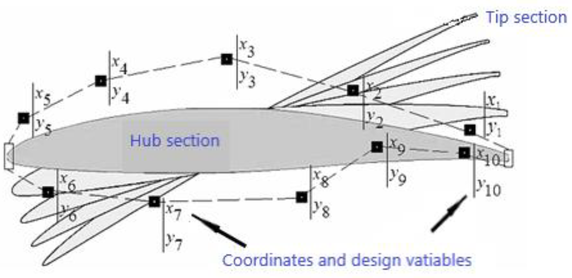
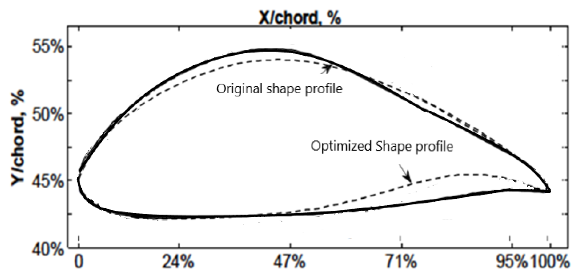
A comparison of the complete airfoil geometry was carried out, as seen in Figure 3. Solid lines depict the geometry of the initial (Datum) unoptimized airfoil. The unoptimized airfoil geometry is shown by the continuous line, while the airfoil shape generated by the AMSP optimizer is shown by the dashed line. The most obvious inference from this graph is that the geometry of the airfoil in the second half of the chord, from maximum thickness to TE, has been significantly affected by the optimization process. An enhanced airfoil shape is produced when three surrogates are combined into an ensemble. This indicates better pressure distribution and greatly increases the lifting force and lowers the drag force of the turbomachinery blades.

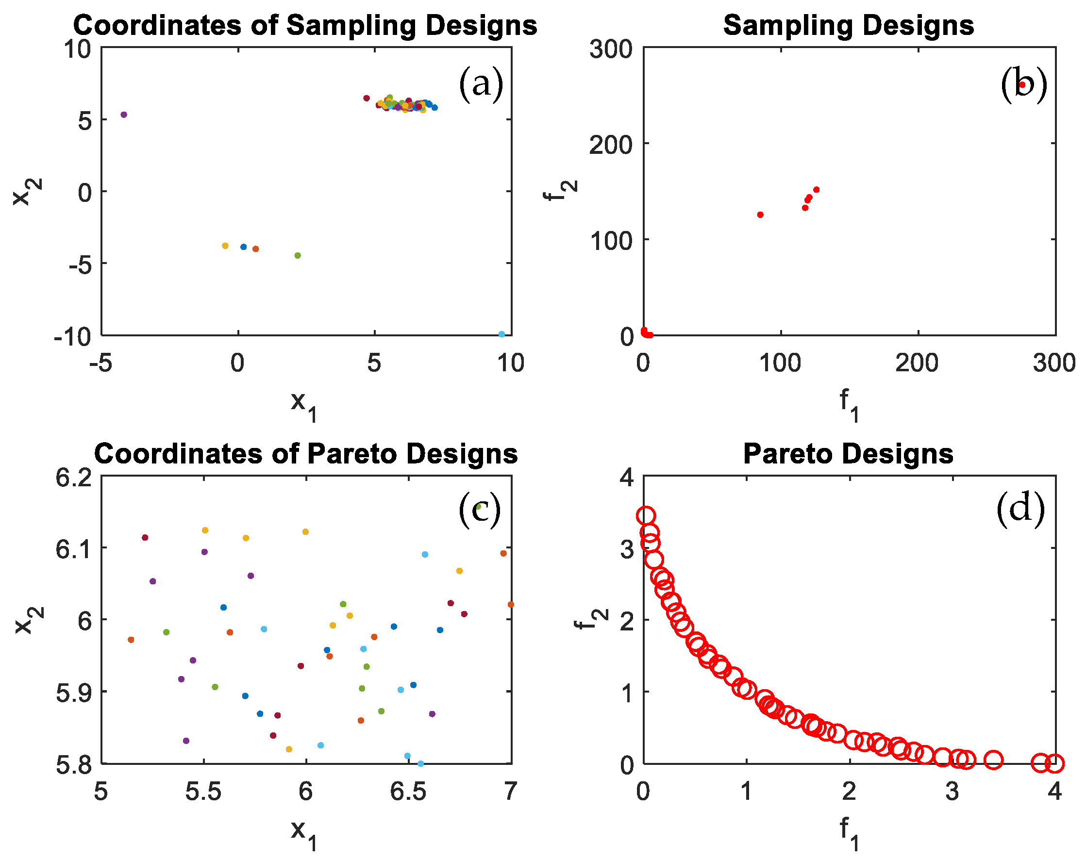
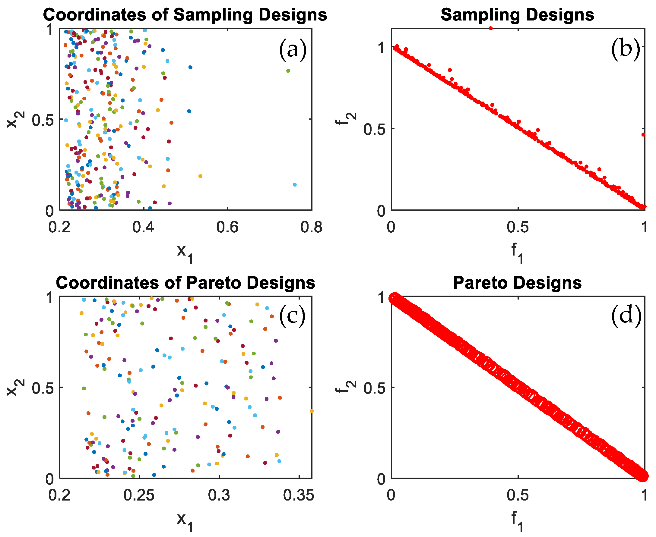
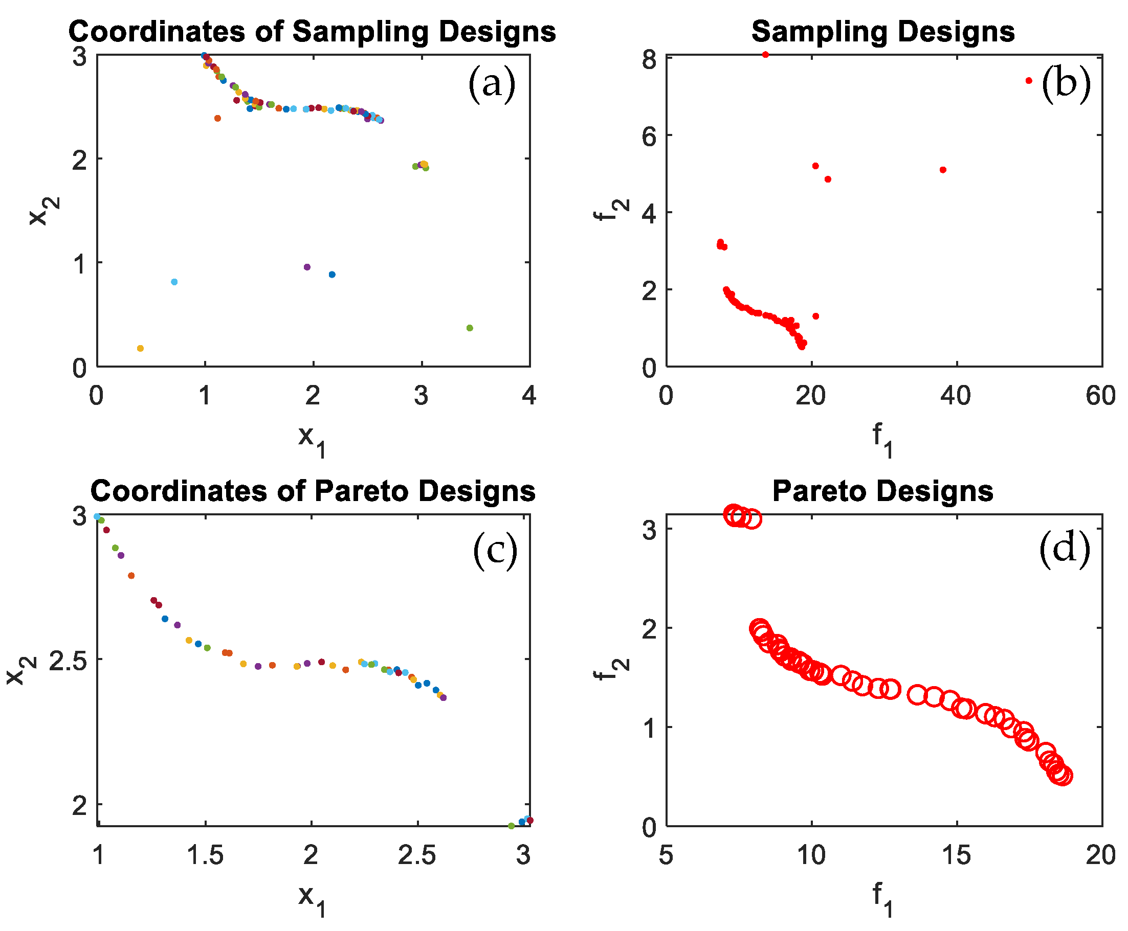
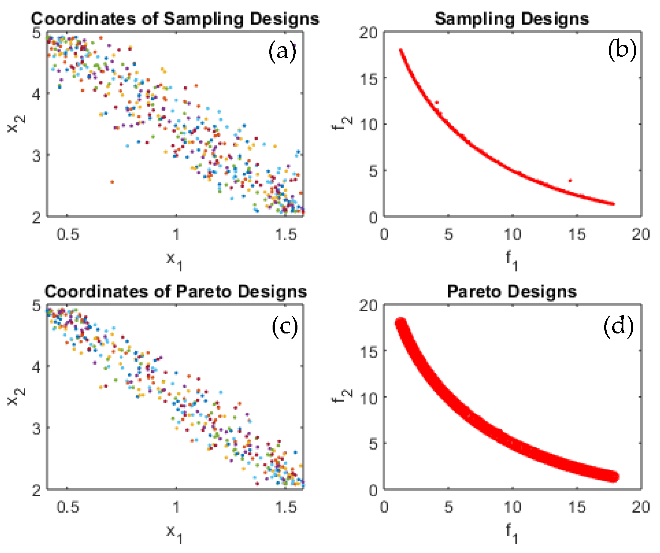
Figure 4, Figure 5, Figure 6 and Figure 7 present the performance space and the evaluated points for test functions F1, F2, T1, T2, and T3 respectively. Figure 4a displays the sampling points coordinates in the feasible design space, Figure 4b shows sampling design at which the sampling design were evaluated using the objective functions. Figure 4c displays the Pareto design coordinates and Figure 4d displays the Pareto frontier after all Pareto coordinates were converged iteration after iteration to form the Pareto frontier. 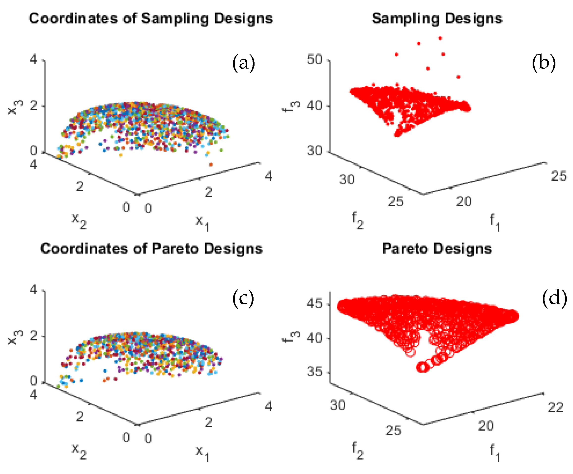The same can be seen in Figure 5, Figure 6, Figure 7 and Figure 8 for test functions F1, F2, T1, T2, and T3. It is quite noticeable that the proposed algorithm successfully converged to optimal Pareto set and successfully identified the Pareto frontier for all tested benchmark multi-objective functions and most importantly for the practical problem, which is the wind turbine blade shape/profile optimization. The algorithm was capable of identifying the Pareto frontier for a real-life practical problem, seen in Figure 8, with three objective functions and 40 design variables. By identifying the optimal design variables $x_1, y_1$, …, $x_{10}, y_{10}$, the optimal airfoil profile was generated that minimizes the loss values $L_1$, $L_2,$ and $L_3$.

Table 3. Summary of test results of AMSP.

Test Function	Number of Iterations		Number of Evaluations		Number of Pareto Set Points
	Range	Median	Range	Median	Range	Median
F1	[23–37]	31	[56–75]	66	[35–48]	44
F2	[20–24]	22	[246–458]	334	[137–357]	232
T1	[15–23]	18	[332–446]	394	[264–363]	321
T2	[27–38]	32	[58–87]	69	[37–46]	42
P1	[219–273]	242	[1170–1294]	1213	[729–793]	760

reports the total number of iterations, the total number of objective function evaluations, and the total number of Pareto points in the ideal Pareto frontier. The efficient Pareto set was successfully identified with a reasonable number of Pareto set points and a low computing cost using RBF, which is devoted to the sample points, and Kriging, which interpolates the sample points and gives good accuracy. Table 3 displays the variation range, median, and Pareto set points for the iterations, function evaluations, and number of iterations.

For each test problem, more than five runs have been completed because LHD creates sample points in the region of interest at random. The best outcome from those several runs is represented by these results. For five distinct runs, the quantity of iterations, total quantity of evaluated points, and quantity of converged frontier points were noted.

It worth mentioning that the task can be completed in a relatively small number of iterations. All the evaluated points are plotted together with the feasible performance space, as shown in Figure 4, Figure 5, Figure 6, Figure 7 and Figure 8 to better observe the accuracy of converged frontier points. The converged frontier points are extremely close to the genuine Pareto frontier, as can be seen by the graphs.

Benchmark test functions were used to compare the proposed algorithm’s performance to that of other MOO algorithms.

Table 4. Performance comparison of multi-objective optimization algorithms.

Test Problem		Number of Iterations		Number of Fun. Evaluations		Number of Pareto Set Points
		Range	Median	Range	Median	Range	Median
F1	AMSP	[23–37]	31	[56–75]	66	[35–48]	44
	PSP	[21–35]	33	[58–79]	68	[36–44]	42
	MOGA	[520–710]	480	[919–1087]	995	[20–24]	22
F2	AMSP	[20–24]	22	[246–458]	334	[137–357]	232
	PSP	[22–24]	23	[260–440]	339	[151–360]	241
	MOGA	[492–780]	503	[1060–1313]	1197	[112–126]	119
T1	AMSP	[15–23]	18	[332–446]	394	[264–363]	321
	PSP	[17–23]	20	[356–476]	400	[33–42]	37
	MOGA	[310–316]	313	[16,246–20,174]	18,841	[19–22]	21
T2	AMSP	[27–38]	32	[58–87]	69	[37–46]	42
	PSP	[52–88]	70	[55–83]	71	[29–44]	35
	MOGA	[418–489]	450	[19,900–22,446]	21,000	[17–21]	19
P1	AMSP	[219–273]	242	[1170–1294]	1213	[729–793]	760
	PSP	[240–264]	246	[1210–1290]	1246	[604–616]	606
	MOGA	[620–980]	800	[310,200–360,900]	33,555	[14–18]	16

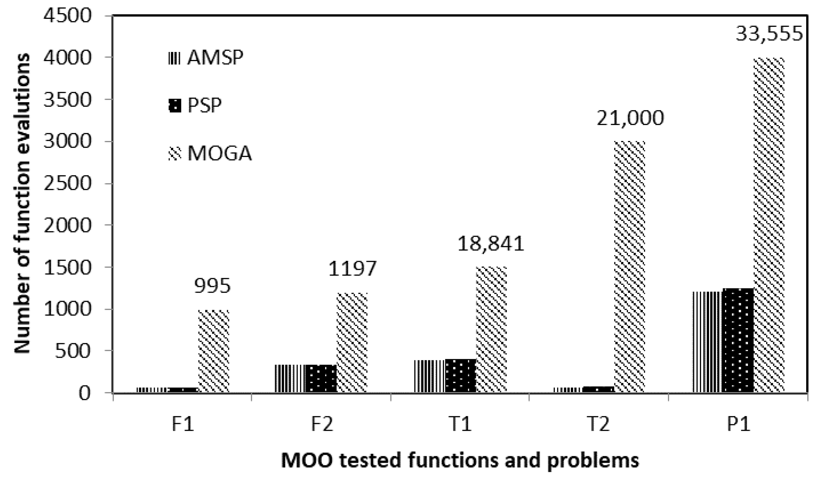
AMSP = Automated Multiobjective Surrogate Based Pareto Finder; PSP = Pareto Set Pursuing’ MOGA = Mulitiobjective Genetic Algorithm

shows that AMSP outperforms the other MOO techniques, such as Pareto Set Pursuing (PSP) and Multi-objective Optimization Genetic Algorithm (MOGA). In terms of the number of fitness evaluations, AMSP outperformed the other algorithms in terms of efforts and resources needed. In addition, the cost of computation was lowered reflected in reduction of number of function evaluations and computation time. Furthermore, when AMSP was utilized, more Pareto set points were obtained. As a result, a more accurate and smoother Pareto border was identified.

The reduction in computation cost is reflected in a smaller number of fitness function evaluations, as seen in Figure 9. In terms of the number of fitness tests required to determine the Pareto optima, AMSP is slightly better than PSP but far better than MOGA. This suggests that AMSP is suitable for complex optimization problems and black box functions, as well as practical engineering applications, due to its ability to handle the burden of effectively exploiting the design space and simulating expensive fitness functions with inexpensive surrogates that can be easily evaluated with fewer resources.

7. Conclusions

A novel and new multi-objective optimization algorithm for identifying the Pareto frontier has been proposed. To find the best Pareto frontier for expensive and black box functions, the suggested algorithm AMSP automatically selects and fits the suitable surrogate approximation model based on RMSE values. Without prior knowledge of the target function, AMSP provides decision makers with a Pareto set for choices. Even if the frontier surface is highly nonlinear or discontinuous, AMSP algorithm can produce solutions that reflect the full Pareto-optimal frontier. With fewer efforts, resources, and expensive function evaluations, AMSP can identify the best Pareto frontier for all tested benchmark test functions with less computational cost and resources. To test the suggested algorithm and show its benefits and drawbacks, a variety of multi-objective benchmark test problems and a practical engineering multi-objective application were examined. The obtained results demonstrated that AMSP could identify the Pareto frontier with comparably good accuracy. When compared against other MOO algorithms, the newly suggested algorithm produced promising outcomes.