
Simulation of Low-Speed Buoyant Flows with a Stabilized Compressible/Incompressible Formulation: The Full Navier–Stokes Approach versus the Boussinesq Model


Abstract
1. Introduction
2. Two Models for Low-Speed Buoyant Flows
2.1. Generalized Liquid/Gas Model
- (i)
- This model has some non-standard features with respect to the usual approaches employed to simulate buoyancy-driven flows. Following the unified approach in [19,20], the present model is based on the conservative form of the transport equations, and it uses the total energy equation instead of the temperature equation.
- (ii)
- This model is valid for any temperature gradient (or temperature difference between walls), as long as the equations of state and the constitutive relationships hold. Compare to the Boussinesq model, which holds up to relative temperature variations of about 10%.
- (iii)
- As shown in [19,20,22,23], this model is endowed with the correct second law of thermodynamics, which stems from the entropy production of the Navier–Stokes equations. This is especially relevant, since many of the models for buoyancy-driven flows violate this principle [24,25]. Furthermore, in the present model, the flow divergence may be non-vanishing; therefore, it is not approximated to be zero, as in the Boussinesq model.
- (iv)
- The total energy equation may be replaced by the internal energy equation or another expression for the temperature equation. However, in order for the model to be entropy consistent, the temperature or energy equation has to retain all the terms, for instance, the dissipation function and the power expansion term (see [3] for other forms of the energy or temperature equations that are consistent). These pitfalls were shown in [24,25] for many usual models employed in the simulation of buoyant flows.
- (v)
- A typical equation of state for a liquid is that the density is only a function of temperature, i.e., . In this case, the equations are termed as the acoustically filtered Navier–Stokes equations [4].
2.2. Boussinesq Approximation
Entropy Production
- (i)
- Note that the entropy production of the buoyant terms in the Boussinesq model should cancel, because gravity is a conservative field. Indeed, this is satisfied if the same buoyancy model is applied to the momentum and energy equations. This is the case of the model presented in this paper. However, there are implementations that do not respect entropy production [24,25]. This is an important trait for physical and numerical reasons. From a numerical point of view, methods can inherit stability from the discrete second law of thermodynamics. From a physical point of view, if the system of equations does not respect the second law of thermodynamics, its solutions are physically wrong [23].
- (ii)
- Note, with this set of equations, the velocity divergence does not appear explicitly in the total energy equation, and, therefore, this model does not suffer the entropy production pitfall of other methods, in which the expansion power appears in the temperature or internal energy equation [24,25]. Indeed, if this is the case, on the one side, the velocity divergence of the Boussinesq model is zero, whereas the real divergence does not cancel due to the changes of density.
- (iii)
- When using the internal energy equation or the temperature equation, the viscous dissipation and power expansion terms should be retained for consistency. As mentioned above, there are models that do not retain these terms.
3. Stabilized Formulation
4. Numerical Example Preliminaries
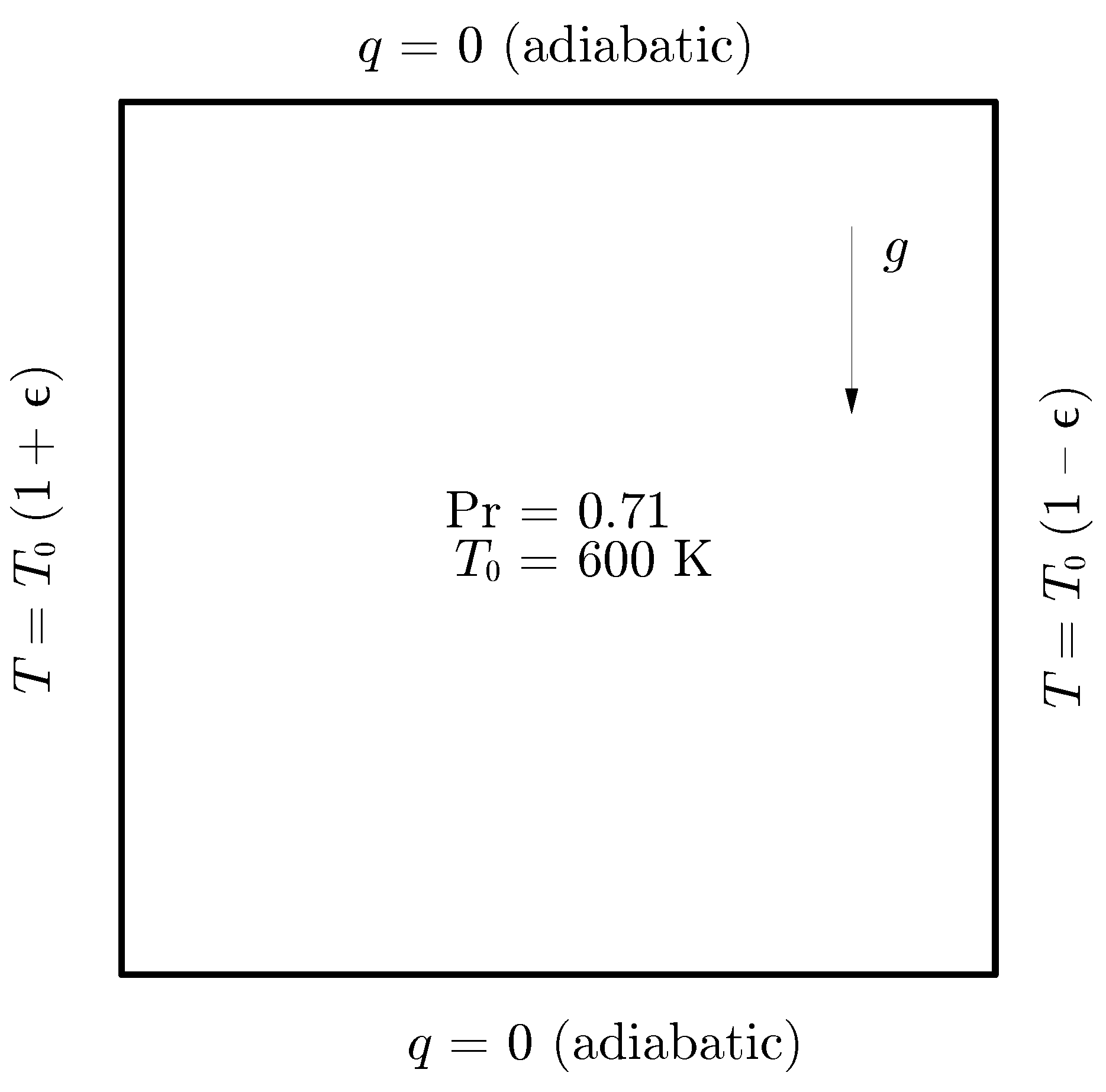
5. Buoyancy-Driven Square Cavity
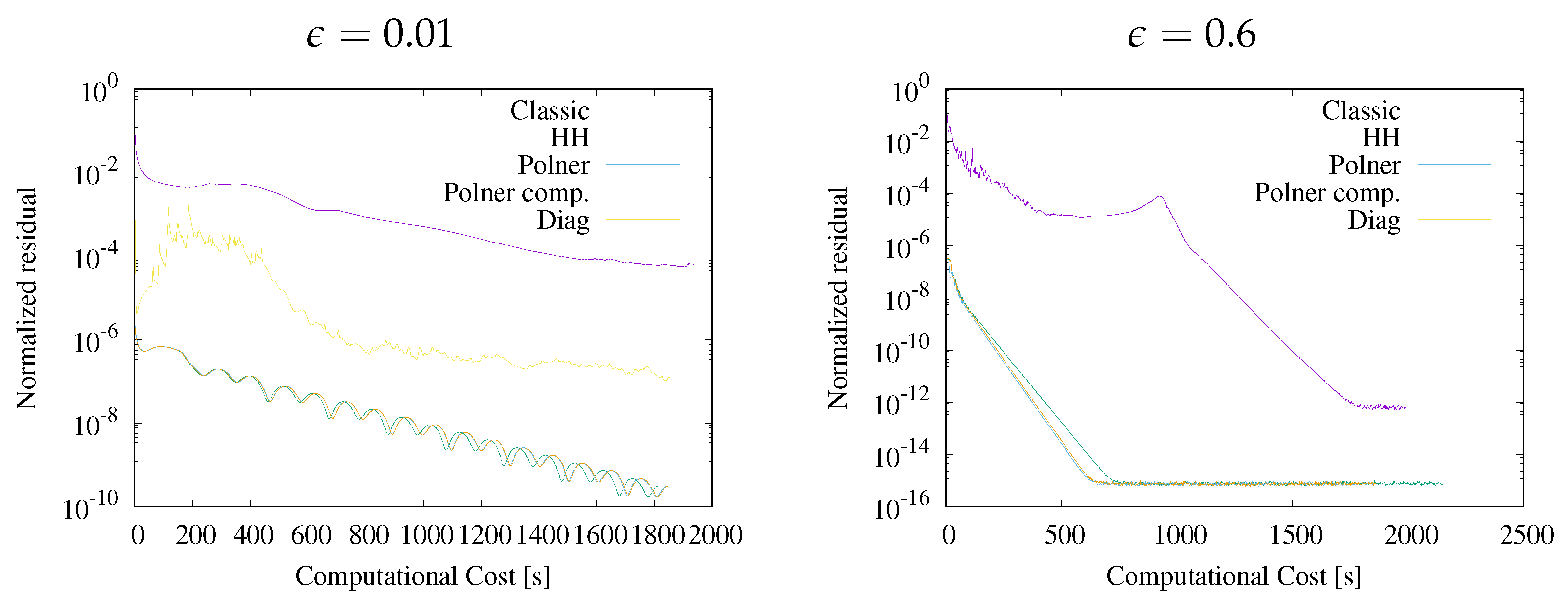
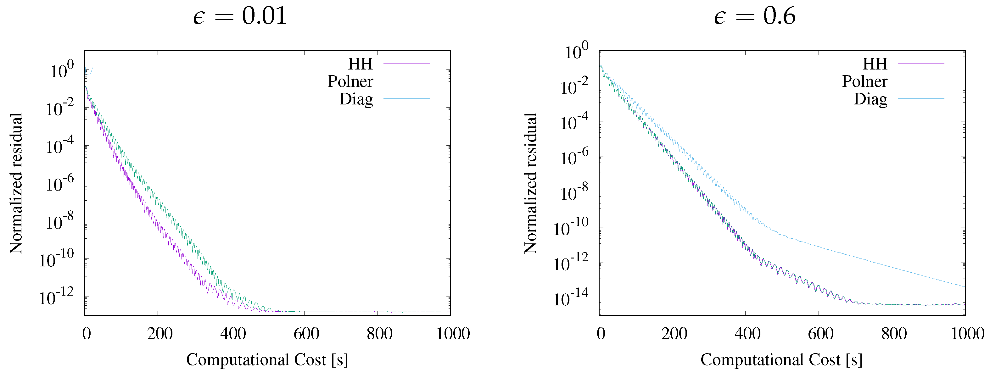
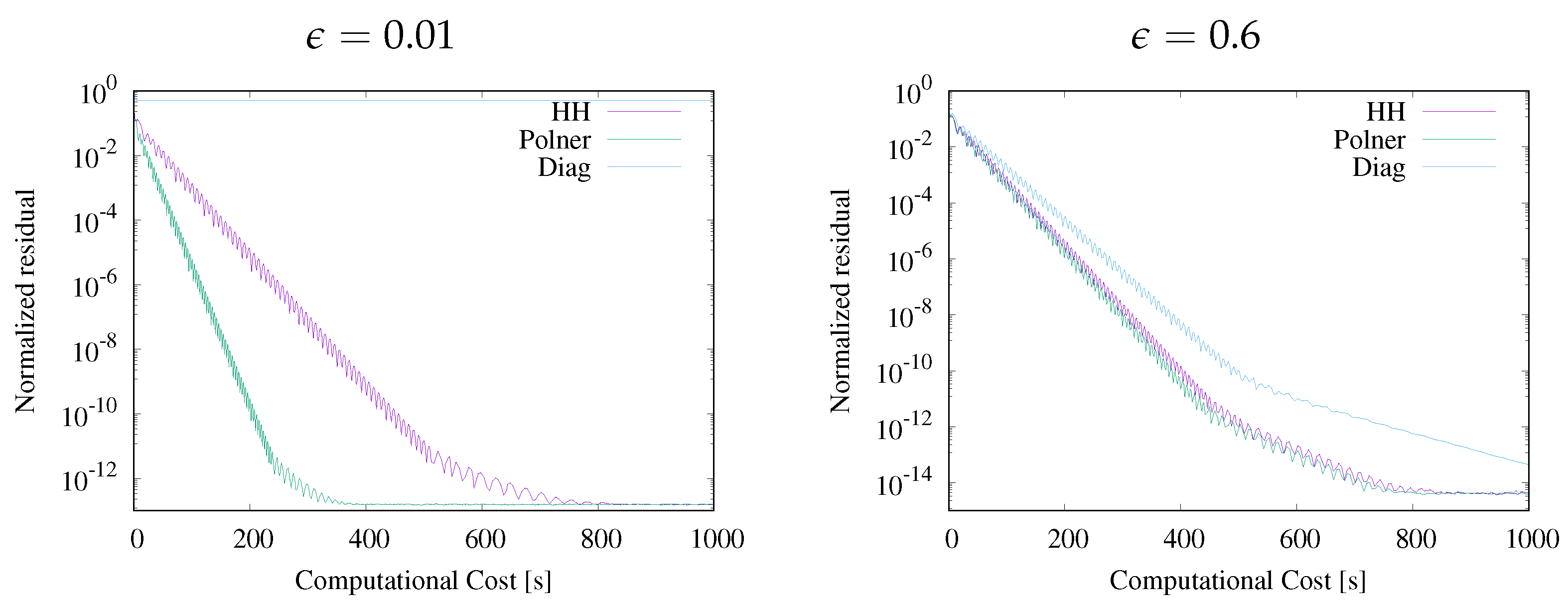
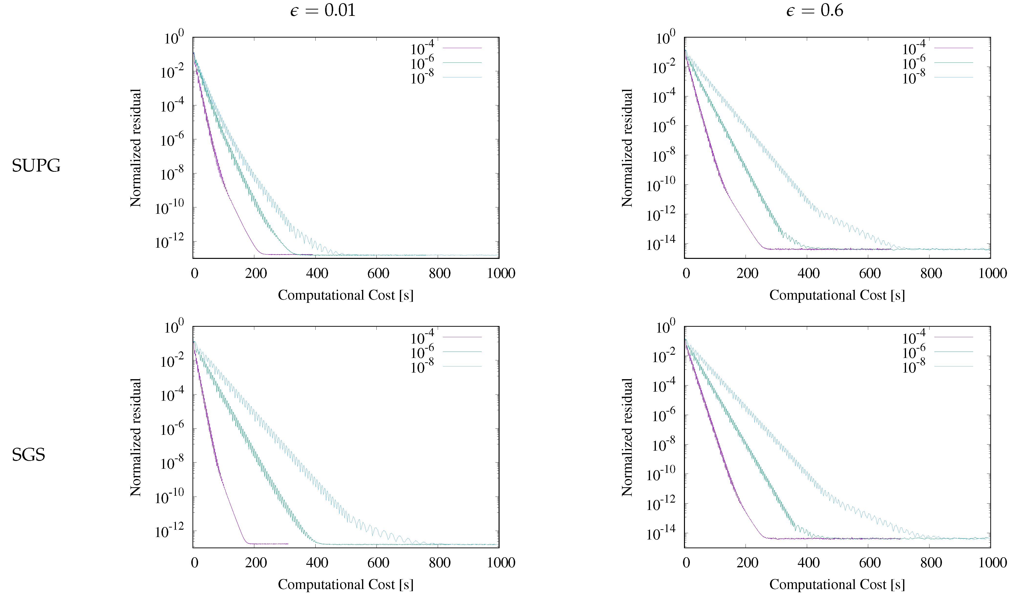
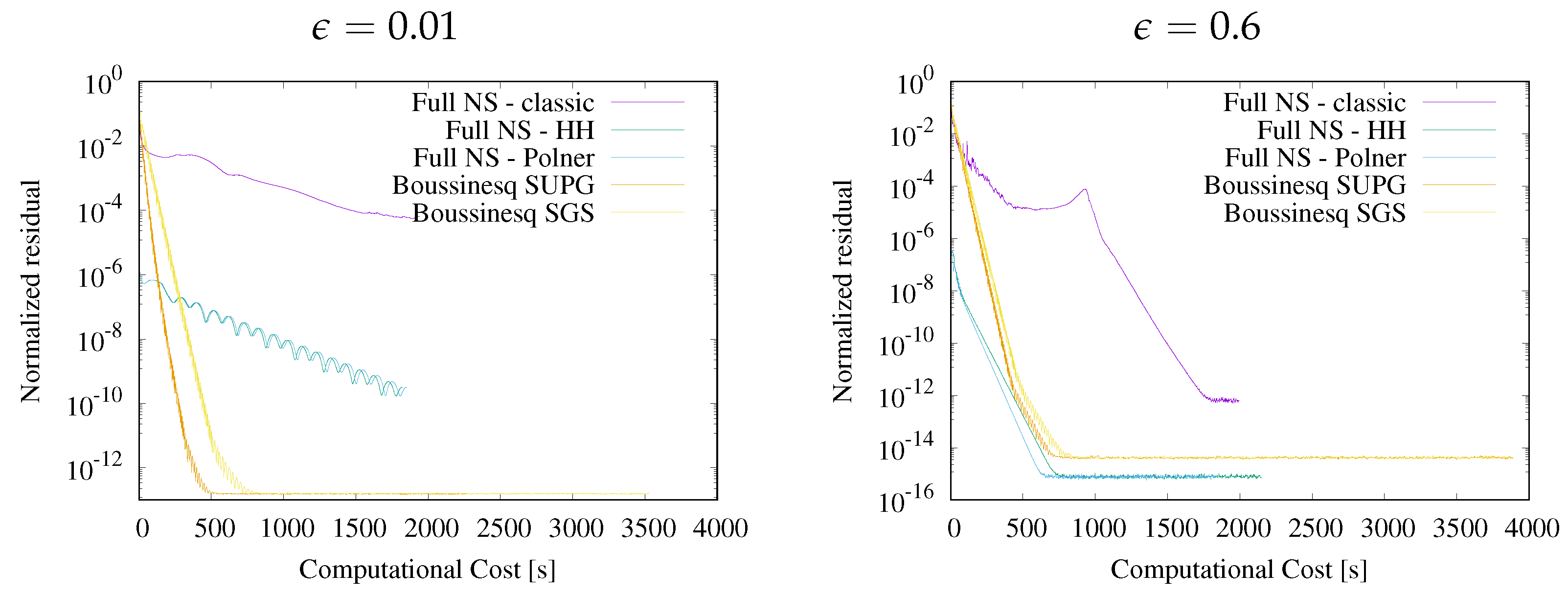
5.1. Residual Convergence Analysis
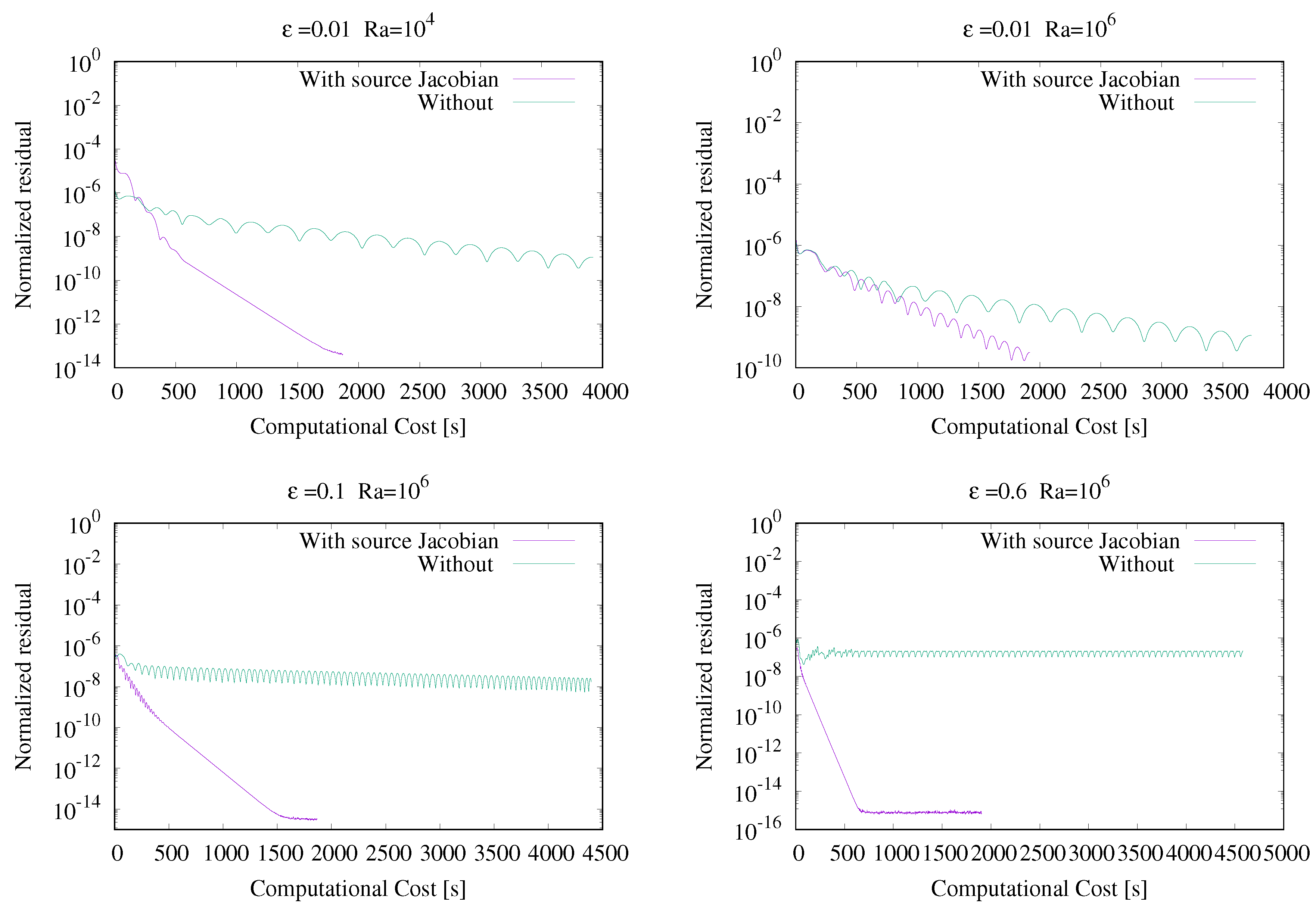
5.2. Relevance of the Body-Force Term within the Full Navier–Stokes Tangent Matrix
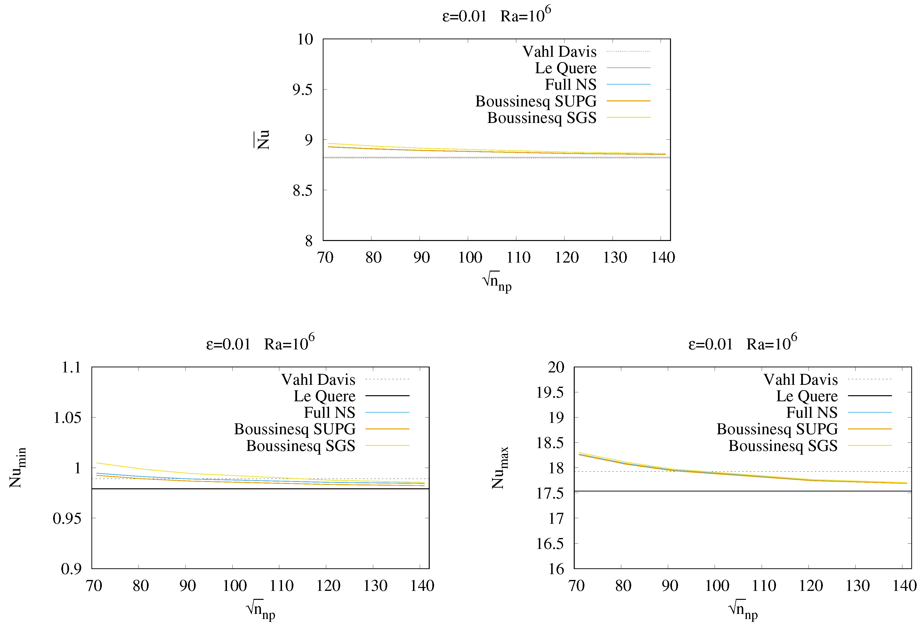
5.3. Case , , Constant Viscosity
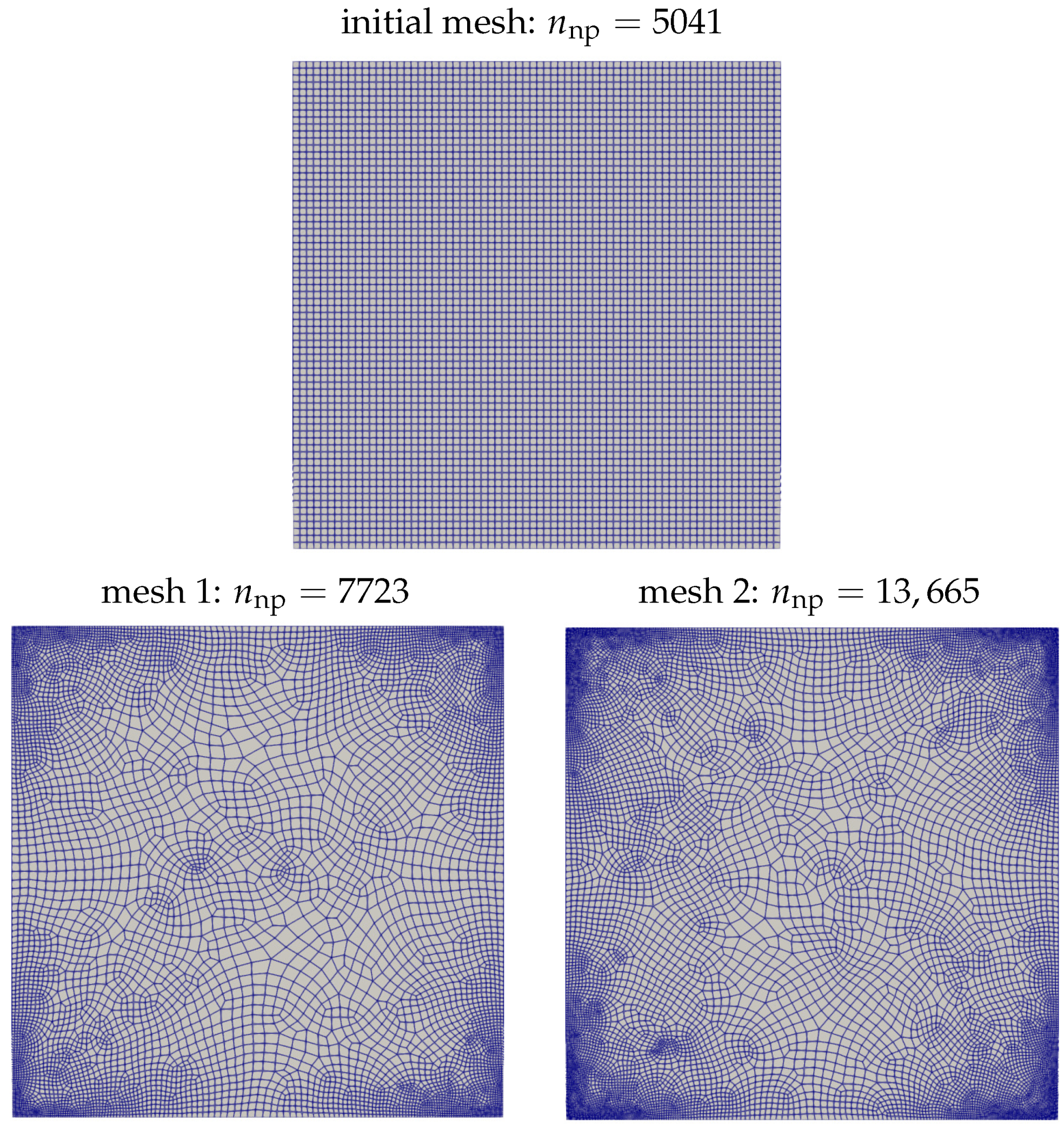
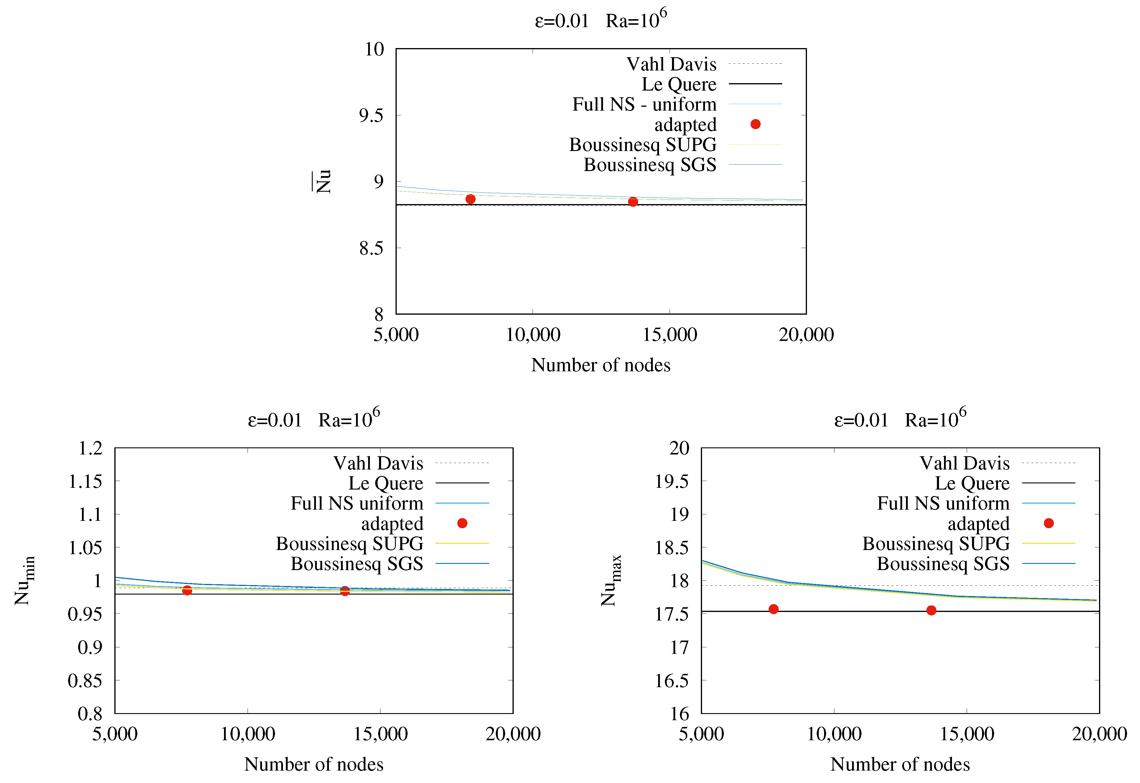
5.4. Case , , Constant Viscosity with Adaptivity
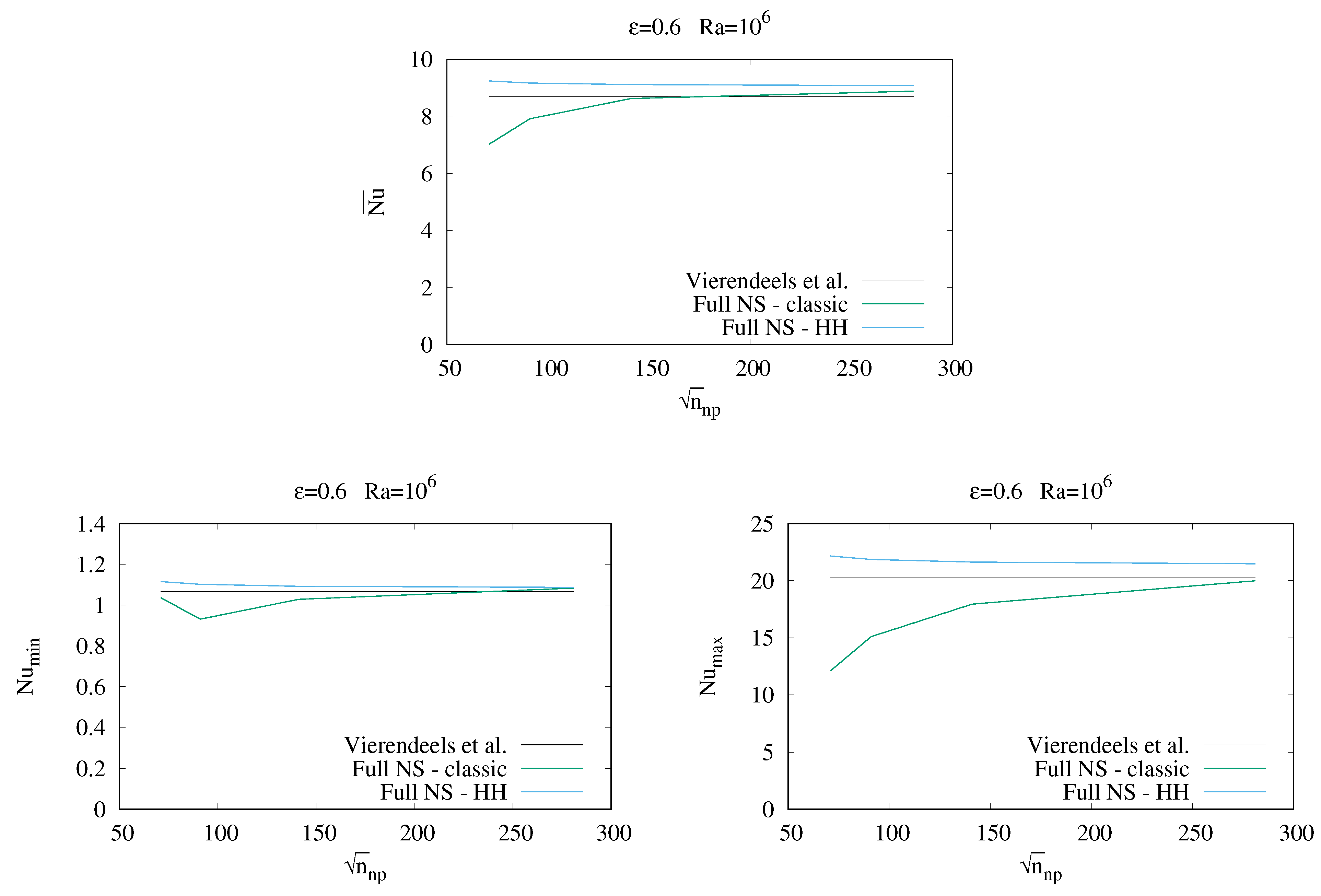
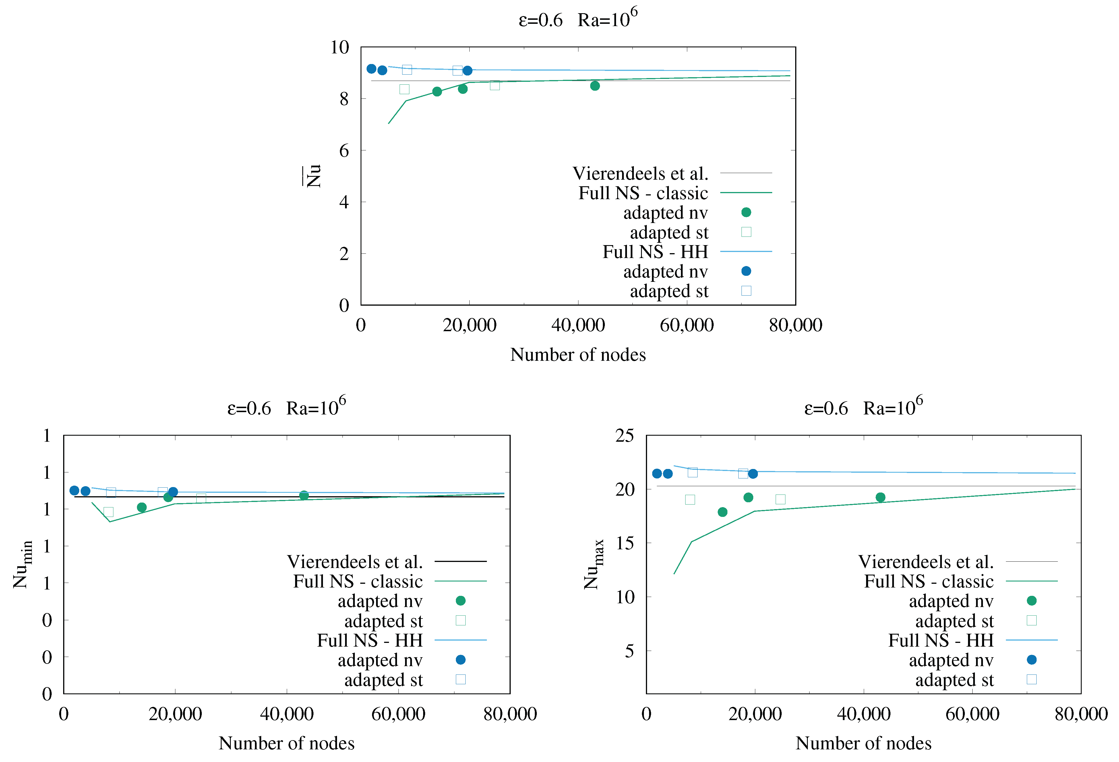
5.5. Case , , Sutherland Viscosity
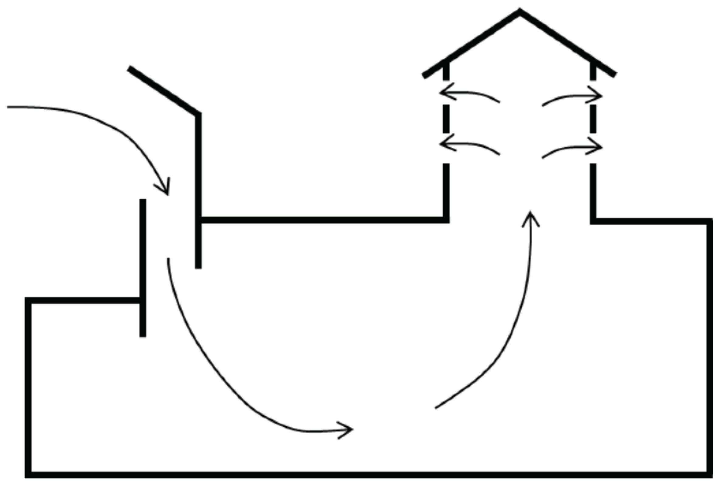
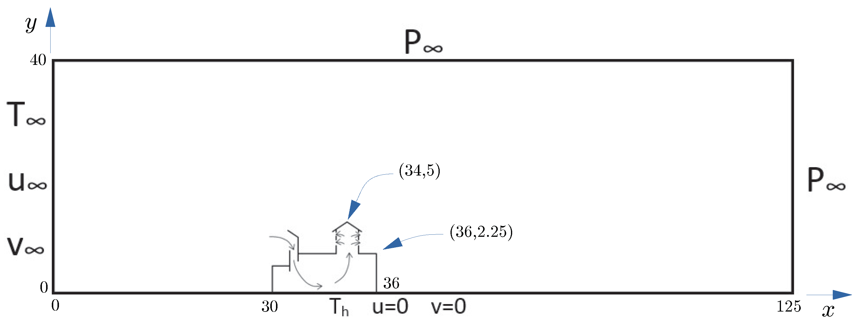
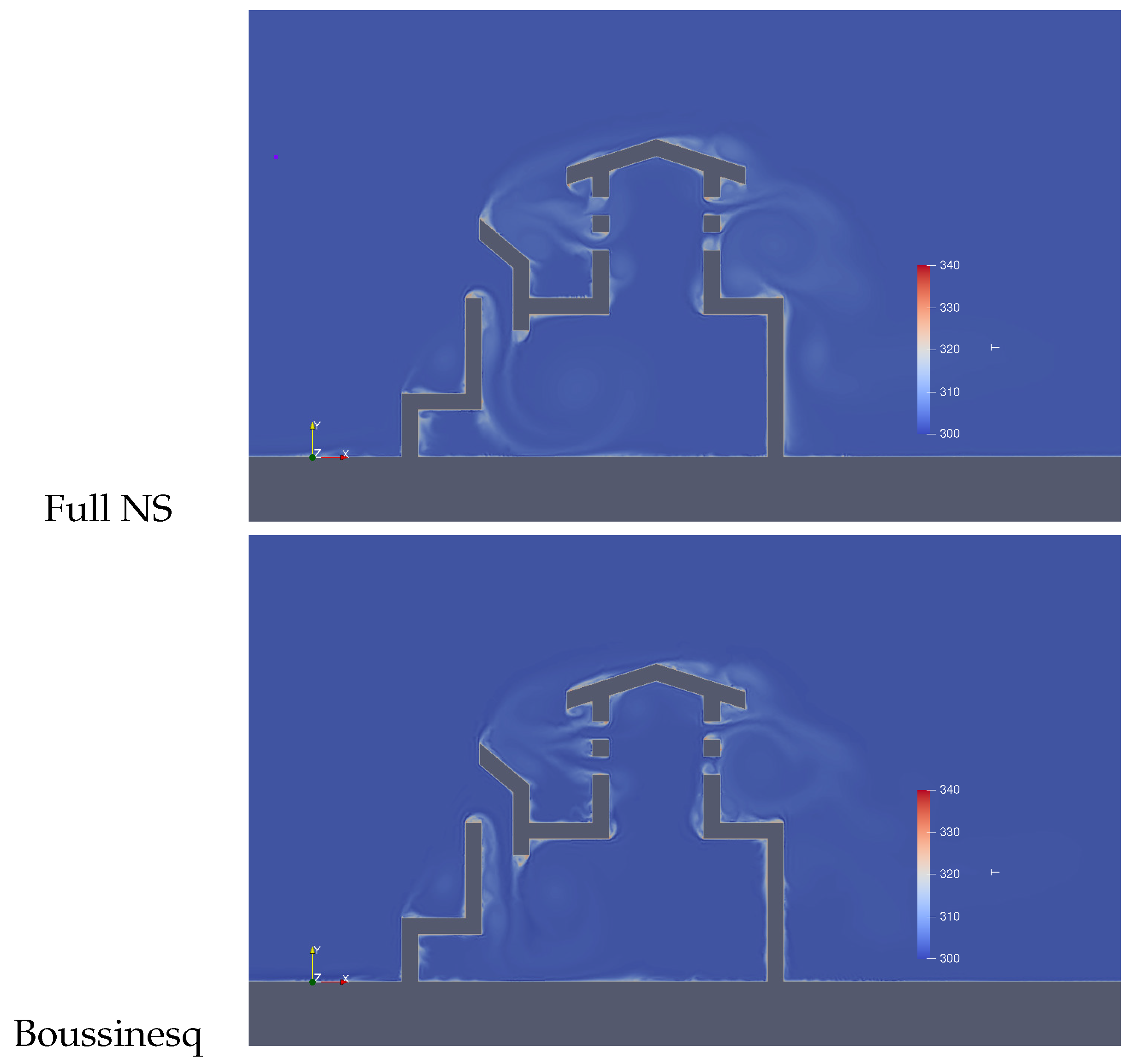
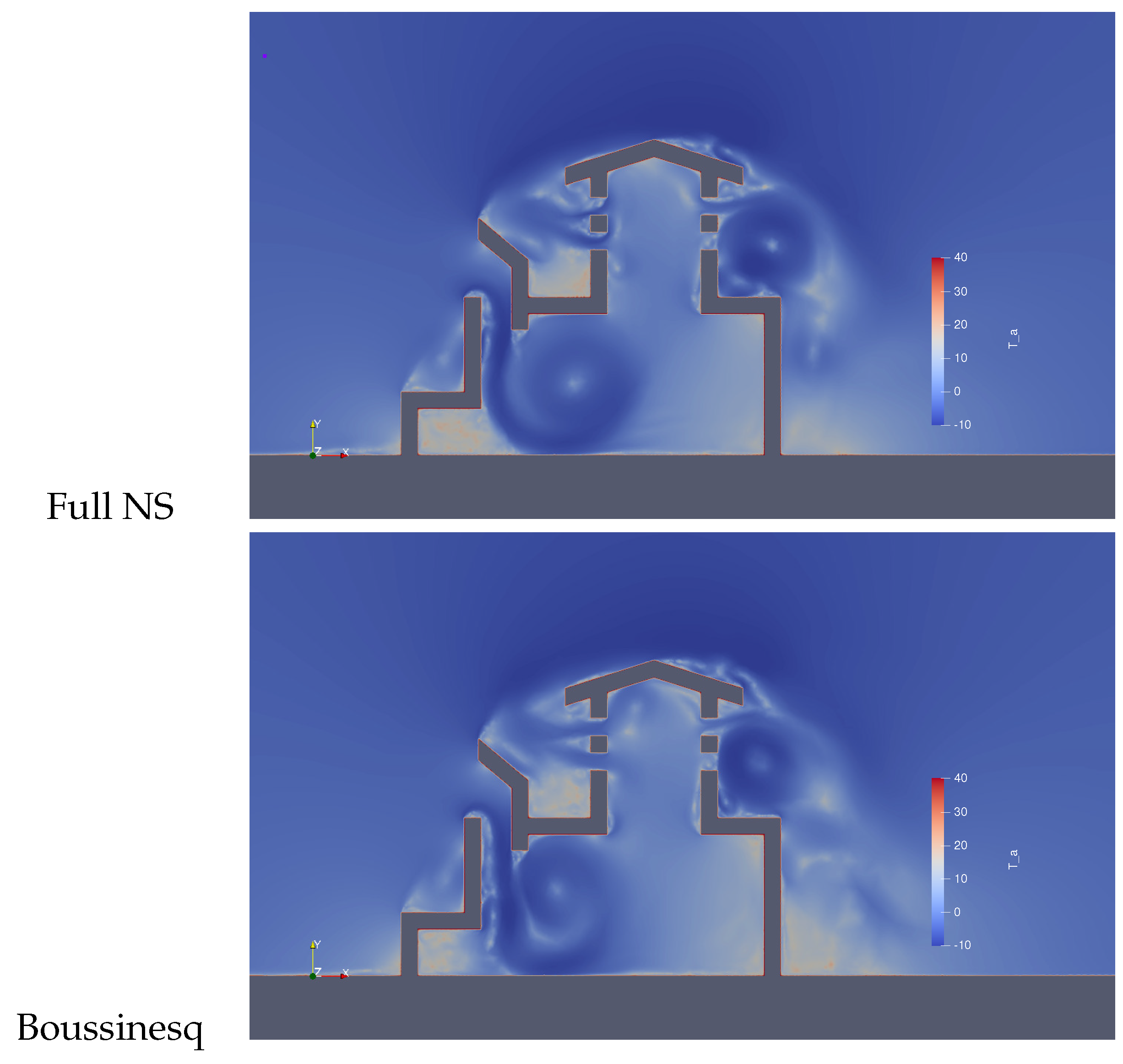
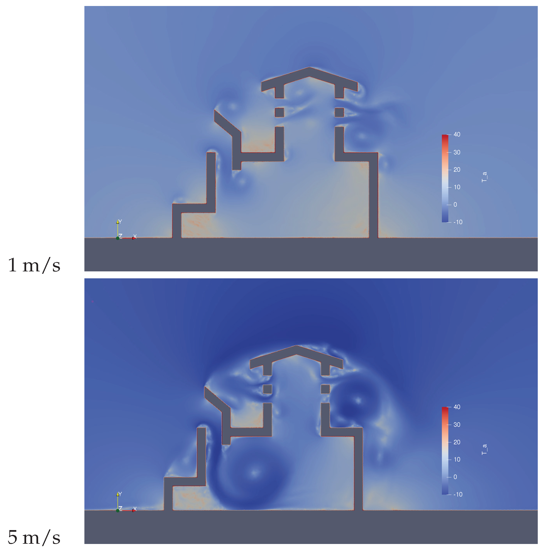
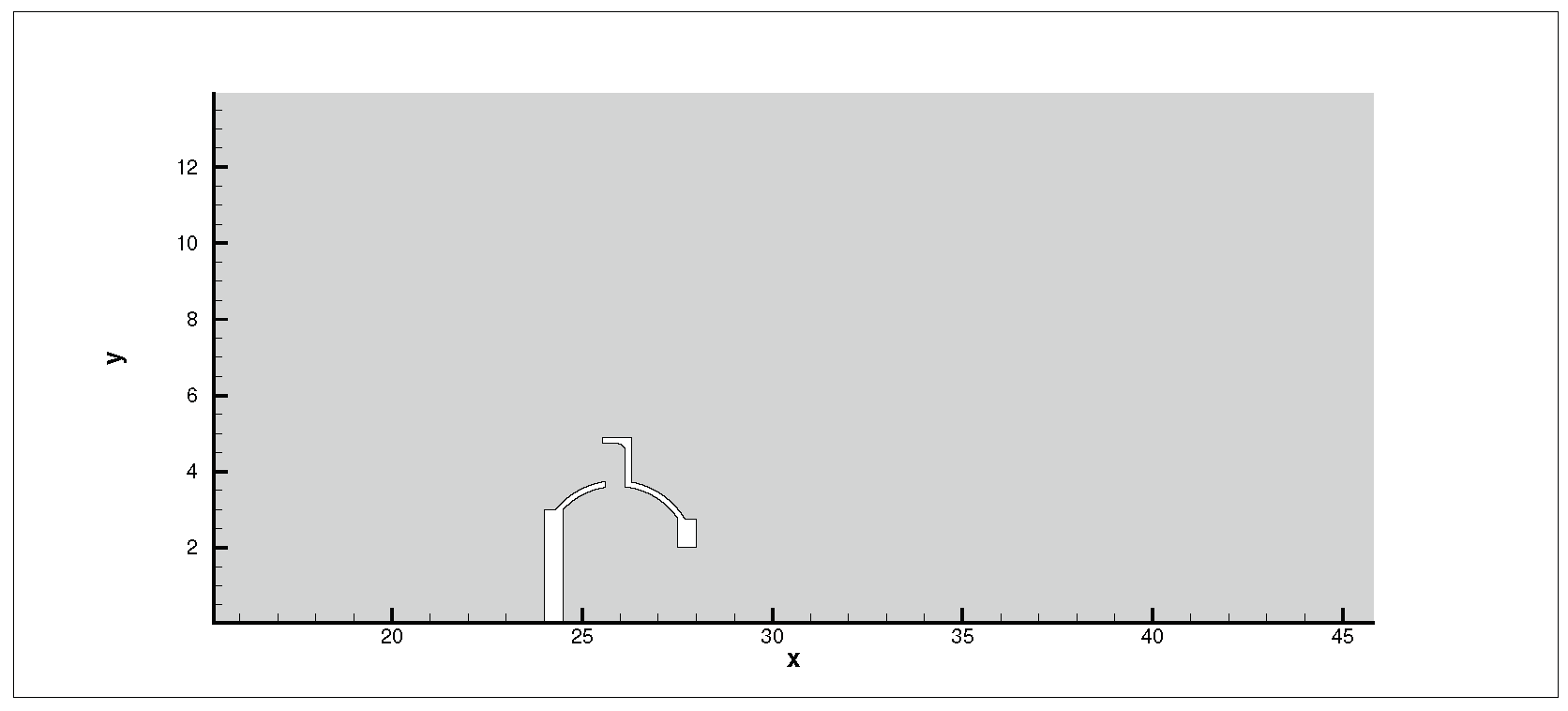
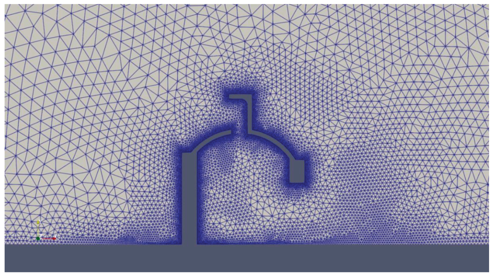
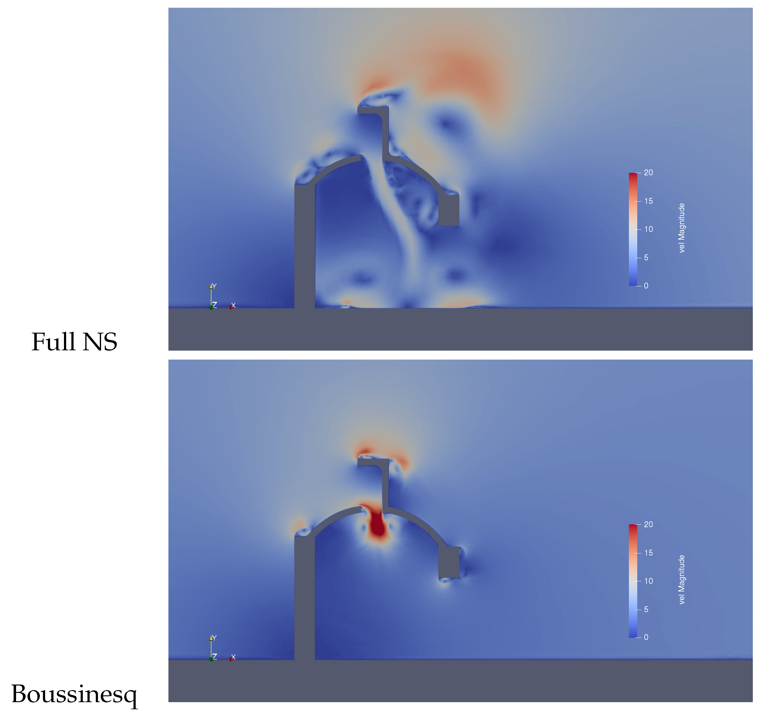
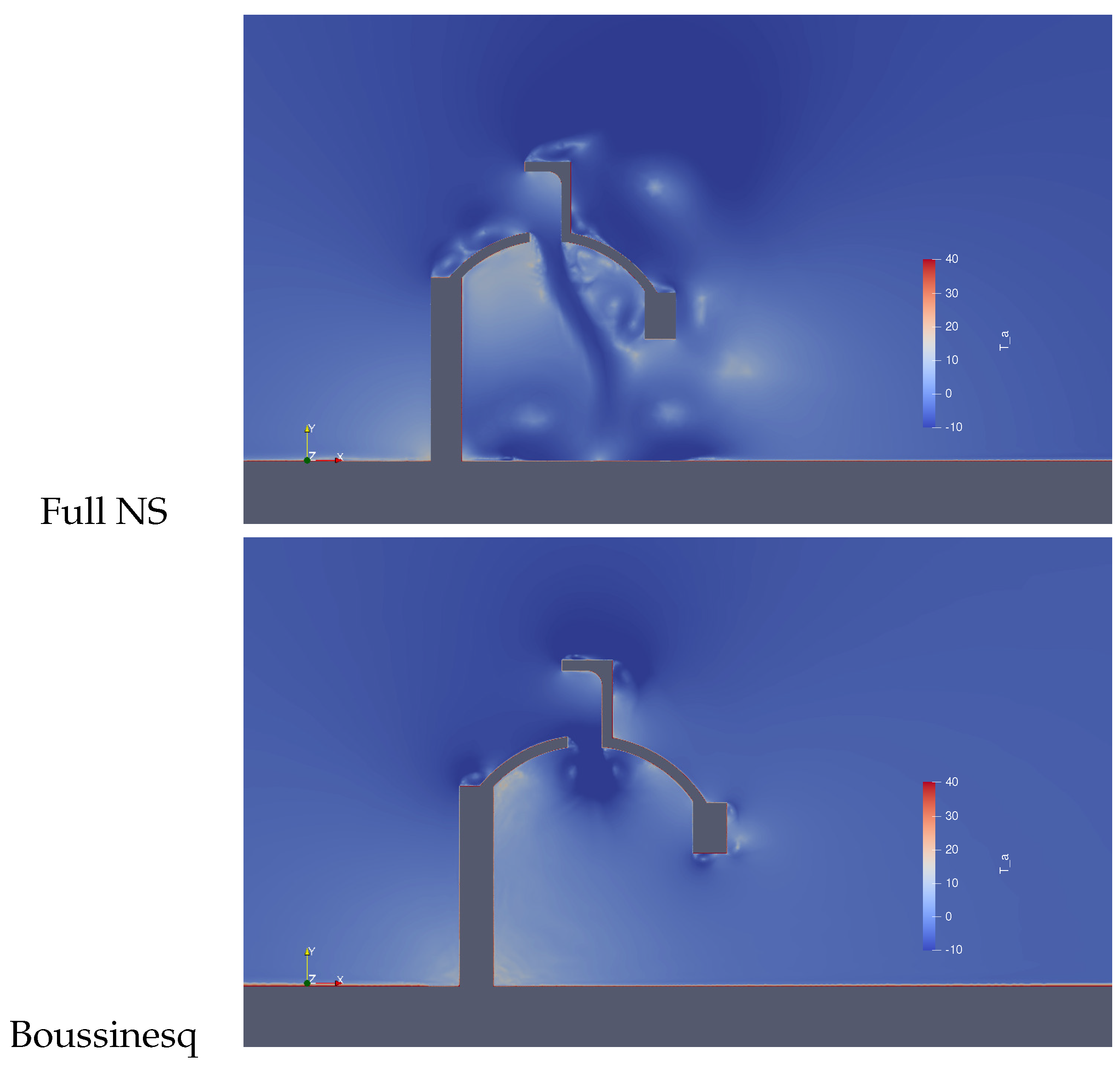
6. Wind Towers
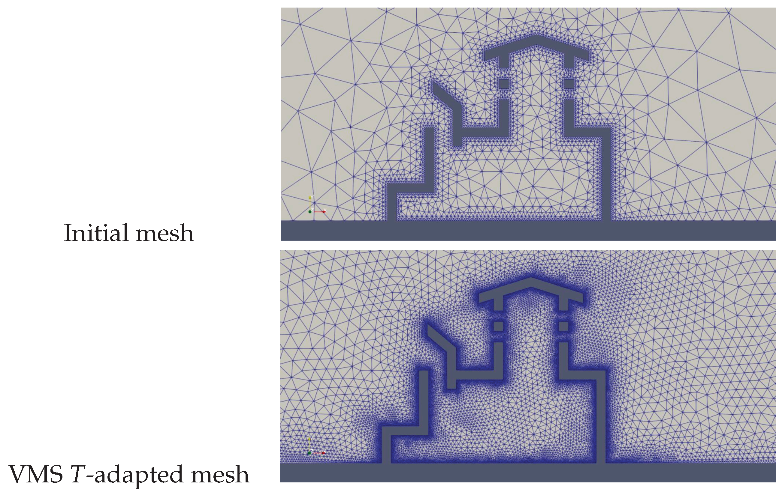
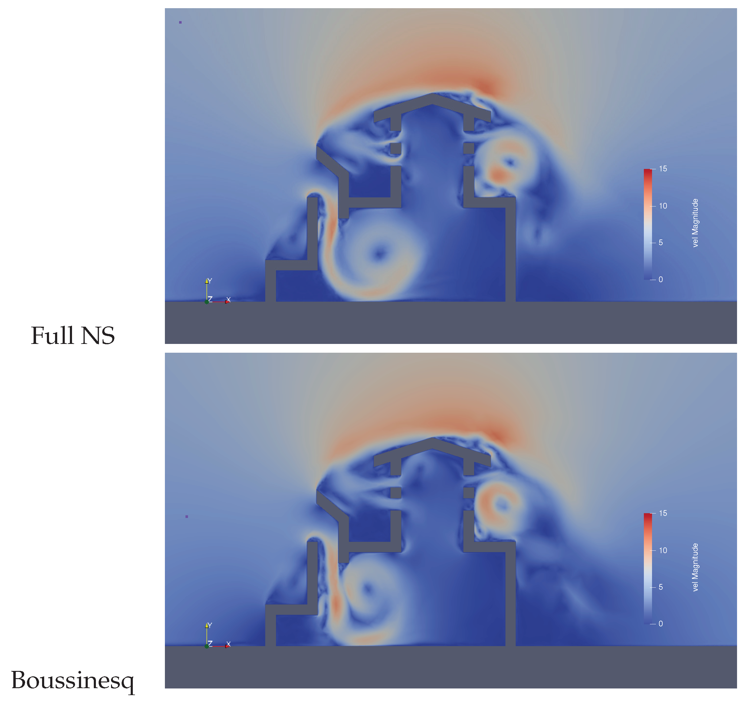
6.1. Application: Wind Tower 1
6.2. Wind Tower 2
7. Conclusions
Author Contributions
Funding
Institutional Review Board Statement
Informed Consent Statement
Data Availability Statement
Acknowledgments
Conflicts of Interest
Appendix A. Structure of the Stabilization Matrices
Appendix B. Jacobians of the Body Force Term
Appendix B.1. Full Navier–Stokes Equations
Appendix B.2. Boussinesq Model
References
- Baker, A.; Williams, P.; Kelso, R. Development of a robust finite element CFD procedure for predicting indoor room air motion. Build. Environ. 1994, 29, 261–273. [Google Scholar] [CrossRef]
- Lube, G.; Knopp, T.; Rapin, G.; Gritzki, R.; Rösler, M. Stabilized finite element methods to predict ventilation efficiency and thermal comfort in buildings. Int. J. Numer. Methods Fluids 2008, 57, 1269–1290. [Google Scholar] [CrossRef]
- Hauke, G. An Introduction to Fluid Mechanics and Transport Phenomena; Springer Science+Business Media, B.V.: Berlin/Heidelberg, Germany, 2008. [Google Scholar]
- Martinez, M.; Gartling, D. A finite element method for low-speed compressible flows. Comput. Methods Appl. Mech. Eng. 2004, 193, 1959–1979. [Google Scholar] [CrossRef]
- Gresho, P.; Sutton, S. Application of the FIDAP code to the 8:1 thermal cavity problem. Int. J. Numer. Methods Fluids 2002, 40, 1083–1092. [Google Scholar] [CrossRef]
- du Toit, C. A segregated finite element solution for non-isothermal flow. Comput. Methods Appl. Mech. Eng. 2000, 182, 457–481. [Google Scholar] [CrossRef]
- Tezduyar, T.E.; Ramakrishnan, S.; Sathe, S. Stabilized formulations for incompressible flows with thermal coupling. Int. J. Numer. Methods Fluids 2008, 57, 1189–1209. [Google Scholar] [CrossRef]
- Principe, J.; Codina, R. A stabilized finite element approximation of low speed thermally coupled flows. Int. J. Numer. Methods Heat Fluid Flow 2008, 18, 835–867. [Google Scholar] [CrossRef][Green Version]
- Ryzhakov, P.; Rossi, R.; Oñate, E. An algorithm for the simulation of thermally coupled low speed flow problems. Int. J. Numer. Methods Fluids 2012, 70, 1–19. [Google Scholar] [CrossRef]
- Benitez, M.; Bermudez, A. A second order characteristics finite element scheme for natural convection problems. J. Comput. Appl. Math. 2011, 235, 3270–3284. [Google Scholar] [CrossRef]
- Gravemeier, V.; Wall, W. Residual-based variational multiscale methods for laminar, transitional and turbulent variable-density flow at low Mach number. Int. J. Numer. Methods Fluids 2011, 65, 1260–1278. [Google Scholar] [CrossRef]
- Yan, J.; Korobenko, A.; Tejada-Martinez, A.; Golshan, R.; Bazilevs, Y. A new variational multiscale formulation for stratified incompressible turbulent flows. Comput. Fluids 2017, 158, 150–156. [Google Scholar] [CrossRef]
- Zhu, L.; Masud, A. Residual-based closure model for density-stratified incompressible turbulent flows. Comput. Methods Appl. Mech. Eng. 2021, 386, 113931. [Google Scholar] [CrossRef]
- Codina, R.; Principe, J. Dynamic subscales in the finite element approximation of thermally coupled incompressible flows. Int. J. Numer. Methods Fluids 2007, 54, 707–730. [Google Scholar] [CrossRef]
- Codina, R.; Principe, J.; Avila, M. Finite element approximation of turbulent thermally coupled incompressible flows with numerical sub-grid scale modelling. Int. J. Numer. Methods Heat Fluid Flow 2010, 20, 492–516. [Google Scholar] [CrossRef]
- Xu, S.; Gao, B.; Hsu, M.C.; Ganapathysubramanian, B. A residual-based variational multiscale method with weak imposition of boundary conditions for buoyancy-driven flows. Comput. Methods Appl. Mech. Eng. 2019, 352, 345–368. [Google Scholar] [CrossRef]
- Principe, J.; Codina, R. Mathematical models for thermally coupled low speed flows. Adv. Theor. Appl. Mech. 2009, 2, 93–112. [Google Scholar]
- Mittal, S.; Tezduyar, T. A unified finite element formulation for compressible and incompressible flows using augmented conservation variables. Comput. Methods Appl. Mech. Eng. 1998, 161, 229–243. [Google Scholar] [CrossRef]
- Hauke, G.; Hughes, T. A unified approach to compressible and incompressible flows. Comput. Methods Appl. Mech. Eng. 1994, 113, 389–395. [Google Scholar] [CrossRef]
- Hauke, G.; Hughes, T. A comparative study of different sets of variables for solving compressible and incompressible flows. Comput. Methods Appl. Mech. Eng. 1998, 153, 1–44. [Google Scholar] [CrossRef]
- Givoli, D.; Flaherty, J.E.; Shephard, M.S. Parallel adaptive finite element analysis of viscous flows based on a combined compressible-incompressible formulation. Int. J. Numer. Methods Heat Fluid Flow 1997, 7, 880–906. [Google Scholar] [CrossRef]
- Chalot, F.; Hughes, T.; Shakib, F. Symmetrization of conservation laws with entropy for high-temperature hypersonic computations. Comput. Syst. Eng. 1990, 1, 459–521. [Google Scholar] [CrossRef]
- Hauke, G.; Landaberea, A.; Garmendia, I.; Canales, J. On the thermodynamics, stability and hierarchy of entropy functions in fluid flow. Comput. Methods Appl. Mech. Eng. 2006, 195, 4473–4489. [Google Scholar] [CrossRef]
- Pons, M.; Quéré, P.L. An example of entropy balance in natural convection, Part 1: The usual Boussinesq equations. Comptes Rendus Méc. 2005, 333, 127–132. [Google Scholar] [CrossRef]
- Pons, M.; Quéré, P.L. An example of entropy balance in natural convection, Part 2: The thermodynamic Boussinesq equations. Comptes Rendus Méc. 2005, 333, 133–138. [Google Scholar] [CrossRef]
- Brooks, A.; Hughes, T. Streamline upwind/Petrov-Galerkin formulations for convection dominated flows with particular emphasis on the incompressible Navier-Stokes equations. Comput. Methods Appl. Mech. Eng. 1982, 32, 199–259. [Google Scholar] [CrossRef]
- Shakib, F.; Hughes, T.; Johan, Z. A new finite element formulation for computational fluid dynamics: X. The compressible Euler and Navier-Stokes equations. Comput. Methods Appl. Mech. Eng. 1991, 89, 141–219. [Google Scholar] [CrossRef]
- Hughes, T.; Franca, L.; Hulbert, G. A new finite element formulation for computational fluid dynamics: VIII. The Galerkin/least-squares method for advective-diffusive equations. Comput. Methods Appl. Mech. Eng. 1989, 73, 173–189. [Google Scholar] [CrossRef]
- Polner, M.; van der Vegt, J.; van Damme, R. Analysis of stabilization operators for Galerkin least-squares discretizations of the incompressible Navier-Stokes equations. Comput. Methods Appl. Mech. Eng. 2006, 196, 982–1006. [Google Scholar] [CrossRef]
- Hauke, G. Simple Stabilizing Matrices for the Computation of Compressible Flows in Primitive Variables. Comput. Methods Appl. Mech. Eng. 2001, 190, 6881–6893. [Google Scholar] [CrossRef]
- Hauke, G.; Landaberea, A.; Garmendia, I.; Canales, J. A Segregated Method for Compressible Flow Computation. Part I.: Isothermal Compressible Flows. Int. J. Numer. Methods Fluids 2005, 47, 271–323. [Google Scholar] [CrossRef]
- Hauke, G.; Landaberea, A.; Garmendia, I.; Canales, J. A Segregated Method for Compressible Flow Computation. Part II.: General Divariant Compressible Flows. Int. J. Numer. Methods Fluids 2005, 49, 183–209. [Google Scholar] [CrossRef]
- Polner, M.; Pesch, L.; van der Vegt, J. Construction of stabilization operators for Galerkin least-squares discretizations of compressible and incompressible flows. Comput. Methods Appl. Mech. Eng. 2007, 196, 2431–2448. [Google Scholar] [CrossRef]
- Costa, G.K.; Lyra, P.R.M. A stabilized finite element formulation to solve high and low speed flows. Commun. Numer. Methods Eng. 2006, 22, 411–419. [Google Scholar] [CrossRef]
- Zhu, L.; Goraya, S.; Masud, A. A Variational Multiscale Method for Natural Convection of Nanofluids. Mech. Res. Commun. 2022. [Google Scholar]
- Taylor, C.; Hughes, T.; Zarins, C. Finite element modeling of blood flow in arteries. Comput. Methods Appl. Mech. Eng. 1998, 158, 155–196. [Google Scholar] [CrossRef]
- Whiting, C.H.; Jansen, K.E. A stabilized finite element method for the incompressible Navier–Stokes equations using a hierarchical basis. Int. J. Numer. Methods Fluids 2001, 35, 93–116. [Google Scholar] [CrossRef]
- Codina, R. Stabilization of incompressibility and convection through orthogonal sub-scales in finite element methods. Comput. Methods Appl. Mech. Eng. 2000, 190, 1579–1599. [Google Scholar] [CrossRef]
- Codina, R. A stabilized finite element method for generalized incompressible flows. Comput. Methods Appl. Mech. Eng. 2001, 190, 2681–2706. [Google Scholar] [CrossRef]
- Codina, R. Stabilized finite element approximation of transient incompressible flows using orthogonal subscales. Comput. Methods Appl. Mech. Eng. 2002, 191, 4295–4321. [Google Scholar] [CrossRef]
- Bazilevs, Y.; Calo, V.; Cottrell, J.; Hughes, T.; Reali, A.; Scovazzi, G. Variational multiscale residual-based turbulence modeling for large eddy simulation of incompressible flows. Comput. Methods Appl. Mech. Eng. 2007, 197, 173–201. [Google Scholar] [CrossRef]
- Bayona, C.; Baiges, J.; Codina, R. Variational multi-scale finite element approximation of the compressible Navier-Stokes equations. Int. J. Numer. Methods Heat Fluid Flow 2016, 26, 1240–1271. [Google Scholar] [CrossRef]
- Xu, F.; Moutsanidis, G.; Kamensky, D.; Hsu, M.C.; Murugan, M.; Ghoshal, A.; Bazilevs, Y. Compressible flows on moving domains: Stabilized methods, weakly enforced essential boundary conditions, sliding interfaces, and application to gas-turbine modeling. Comput. Fluids 2017, 158, 201–220. [Google Scholar] [CrossRef]
- Hughes, T.; Scovazzi, G.; Tezduyar, T. Stabilized methods for compressible flows. J. Sci. Comput. 2010, 43, 343–368. [Google Scholar] [CrossRef]
- Franca, L.; Frey, S. Stabilized finite element methods: II. The incompressible Navier-Stokes equations. Comput. Methods Appl. Mech. Eng. 1992, 99, 209–233. [Google Scholar] [CrossRef]
- de Vahl Davis, G. Natural Convection of Air in a Square Cavity: A Bench Mark Numerical Solution. Int. J. Numer. Methods Fluids 1983, 3, 249–264. [Google Scholar] [CrossRef]
- LeQuéré, P.; Weisman, C.; Paillère, H.; JanVierendeels.; Dick, E.; Becker, R.; Braack, M.; Locke, J. Modelling of Natural Convection Flows with LargeTemperature Differences: A Benchmark Problem for Low MachNumber Solvers. Part 1. Reference Solutions. ESAIM Math. Model. Numer. Anal. 2005, 39, 609–616. [Google Scholar] [CrossRef]
- Mamimid, S.; Guellal, M.; Bouafia, M. Numerical study of natural convection in a square cavity under non-Boussinesq conditions. Therm. Sci. 2016, 20, 1509–1517. [Google Scholar]
- Becker, R.; Braak, M. Solution of a stationary benchmark problem for natural convection with large temperature difference. Int. J. Therm. Sci. 2002, 41, 428–439. [Google Scholar] [CrossRef]
- Heuveline, V. On higher-order mixed FEM for low Mach number flows: Application to a natural convection benchmark problem. Int. J. Numer. Methods Fluids 2003, 41. [Google Scholar] [CrossRef]
- de Vahl Davis, G.; Jones, I. Natural Convection in a square Cavity: A comparison exercise. Int. J. Numer. Methods Fluids 1983, 3, 227–248. [Google Scholar] [CrossRef]
- Vierendeels, J.; Merci, B.; Dick, E. Numerical study of natural convective heat transfer with large horizontal temperature differences. Int. J. Numer. Methods Heat Fluid Flow 2001, 11, 329–341. [Google Scholar] [CrossRef]
- Vierendeels, J.; Merci, B.; Dick, E. Benchmark solutions for the natural convective heat transfer problem in a square cavity with large horizontal temperature differences. Int. J. Numer. Methods Heat Fluid Flow 2003, 13, 1057–1078. [Google Scholar] [CrossRef]
- Paillère, H.; Le LeQuéré, P.; Weisman, C.; Vierendeels, J.; Dick, E.; Braack, M.; Dabbene, F.; Beccantini, A.; Studer, E.; Kloczko, T.; et al. Modelling of Natural Convection Flows with LargeTemperature Differences: A Benchmark Problem for Low MachNumber Solvers. Part 2. Contributions to the 2004 June Conference. ESAIM Math. Model. Numer. Anal. 2005, 39, 617–621. [Google Scholar] [CrossRef]
- Wittschieber, S.; Demkowicz, L.; Behr, M. Stabilized finite element methods for a fully-implicit logarithmic reformulation of the Oldroyd-B constitutive law. J. Non-Newton. Fluid Mech. 2022, 306, 104838. [Google Scholar] [CrossRef]
- Quéré, P.L. Accurate solutions to the square thermally driven cavity at high Rayleigh number. Comput. Fluids 1991, 20, 29–41. [Google Scholar] [CrossRef]
- Hauke, G.; Doweidar, M.H.; Miana, M. Proper intrinsic scales for a-posteriori multiscale error estimation. Comput. Methods Appl. Mech. Eng. 2006, 195, 3983–4001. [Google Scholar] [CrossRef]
- Irisarri, D.; Hauke, G. A posteriori pointwise error computation for 2-D transport equations based on the variational multiscale method. Comput. Methods Appl. Mech. Eng. 2016, 311, 648–670. [Google Scholar] [CrossRef]
- Irisarri, D.; Hauke, G. A posteriori error estimation and adaptivity based on VMS for the incompressible Navier-Stokes equations. Comput. Methods Appl. Mech. Eng. 2021, 373, 113508. [Google Scholar] [CrossRef]
- Hauke, G.; Fuster, D.; Lizarraga, F. Variational multiscale a posteriori error estimation for systems: The Euler and Navier–Stokes equations. Comput. Methods Appl. Mech. Eng. 2015, 283, 1493–1524. [Google Scholar] [CrossRef]
- Hauke, G.; Doweidar, M.H.; Fuentes, S. Mesh adaptivity for the transport equation led by variational multiscale error estimators. Int. J. Numer. Methods Fluids 2011, 69, 1835–1850. [Google Scholar] [CrossRef]
- Ortego, I. Torres de Viento. Relectura Contemporanea de Sistemas Energetivos Pasivos. Master’s Thesis, ETS Arquitectura de Madrid, Madrid, Spain, 2020. [Google Scholar]


| SUPG | GLS | SGS | |
|---|---|---|---|
| Reference Solution | ||||
| vahl Davis [46] | 8.817 | 0.989 | 17.925 | |
| Le Quéré [56] | 8.8252 | 0.97946 | 17.5360 | |
| Vierendeels [52] | 8.8257 | |||
| Masud [35] | 8.81490 | |||
| Present Method | tau | |||
| Full NS | Classic | 8.0833 | 0.803 | 13.932 |
| Full NS | HH | 8.8524 | 0.984 | 17.704 |
| Full NS | Polner | 8.8526 | 0.984 | 17.703 |
| Boussinesq SUPG | HH | 8.8540 | 0.982 | 17.689 |
| Boussinesq SUPG | Polner | 8.8542 | 0.982 | 17.688 |
| Boussinesq SGS | HH | 8.8632 | 0.985 | 17.704 |
| Boussinesq SGS | Polner | 8.8634 | 0.985 | 17.703 |
| Reference Solution | ||||
| Vierendeels et al. [53,54] | 8.6866 | 1.0667 | 20.2704 | |
| Heuveline [50,54] | 8.6861 | 1.0674 | 20.3051 | |
| Becker-Braak [49] | 8.6866 | |||
| Present method | tau | |||
| Full NS | Classic | 8.6227 | 1.027 | 17.940 |
| Full NS | HH | 9.1134 | 1.093 | 21.629 |
| Full NS | Polner | 9.1142 | 1.093 | 21.632 |
Publisher’s Note: MDPI stays neutral with regard to jurisdictional claims in published maps and institutional affiliations. |
© 2022 by the authors. Licensee MDPI, Basel, Switzerland. This article is an open access article distributed under the terms and conditions of the Creative Commons Attribution (CC BY) license (https://creativecommons.org/licenses/by/4.0/).
Share and Cite
Hauke, G.; Lanzarote, J. Simulation of Low-Speed Buoyant Flows with a Stabilized Compressible/Incompressible Formulation: The Full Navier–Stokes Approach versus the Boussinesq Model. Algorithms 2022, 15, 278. https://doi.org/10.3390/a15080278
Hauke G, Lanzarote J. Simulation of Low-Speed Buoyant Flows with a Stabilized Compressible/Incompressible Formulation: The Full Navier–Stokes Approach versus the Boussinesq Model. Algorithms. 2022; 15(8):278. https://doi.org/10.3390/a15080278
Chicago/Turabian StyleHauke, Guillermo, and Jorge Lanzarote. 2022. "Simulation of Low-Speed Buoyant Flows with a Stabilized Compressible/Incompressible Formulation: The Full Navier–Stokes Approach versus the Boussinesq Model" Algorithms 15, no. 8: 278. https://doi.org/10.3390/a15080278
APA StyleHauke, G., & Lanzarote, J. (2022). Simulation of Low-Speed Buoyant Flows with a Stabilized Compressible/Incompressible Formulation: The Full Navier–Stokes Approach versus the Boussinesq Model. Algorithms, 15(8), 278. https://doi.org/10.3390/a15080278