Multifractal Characterization and Modeling of Blood Pressure Signals

Abstract

In this paper, a multi-fractal analysis on a diastolic blood pressure signal is conducted. The signal is measured in a time span of circa one day through the multifractal detrended fluctuation analysis framework. The analysis is performed on asymptotic timescales where complex regulating mechanisms play a fundamental role in the blood pressure stability. Given a suitable frequency range and after removing non-stationarities, the blood pressure signal shows interesting scaling properties and a pronounced multifractality imputed to long-range correlations. Finally, a binomial multiplicative model is investigated showing how the analyzed signal can be described by a concise multifractal model with only two parameters.

1. Introduction

The combination of chaos and, in general, complexity theory and biomedical engineering promotes an in-depth study of biomedical problems and provides new ways for studying physiological signals, whose parameter variations are difficult to describe accurately by classical approaches [1]. Indeed, fractal structures and chaotic dynamics are found in biomedical time series drawn from a wide range of physiological phenomena [2]. In fact, the availability of improved and (often) non-invasive technologies to measure physiological signals, together with powerful frameworks for complex systems analysis, allow an in-depth characterization of the inherent mechanisms underlying the physiological regulation. The study of physiological signals has also gained a lot of attention in the machine learning community, especially in various correlation and predictive studies leading themselves to non-invasive methodologies to detect brain injuries [3,4,5]. Complex physiological rhythms and peculiar fluctuations are widespread within most parts of the biological systems and subsystems, starting from sub-cellular levels to organs or even the entire body. Such fluctuations arise from the combined influences of the fluctuating environment (i.e., the “noise” that is inherent in biological systems) and deterministic, possibly chaotic, mechanisms [6]. Despite the growth of studies in this area, the role of the low and high degree of freedom dynamics within physiological systems is still unclear. However, as opposed to the daily human experience, intrinsic noisy dynamics have been found to be of paramount importance for healthy conditions, especially in fine-grained regulatory mechanisms. These regulation mechanisms are often very complex and act jointly to reach a suitable equilibrium state. As an example, the heartbeat is generated by an autonomous pacemaker in the heart, but its frequency is mediated by the neural activity, which is controlled, in turn, by a large number of different feedback circuits all acting in parallel [6].

Moreover, many physiological signals have been found to possess some appealing properties, such as scale invariance and fractal dynamics, that is, when the structure repeats itself on sub-intervals of the signal. In other words, the following definition holds.

Definition 1

(Scale-invariant signal). A signal $X\left(t\right)$, is said to be scale invariant when it features a power-law behavior such as $X\left(ct\right)=c^{H}X\left(t\right)$, with c being a suitable constant.

The presence of such a family of laws seems to be ubiquitous in nature. The power-law exponent H, in general, describes the particular kind of fractal and scale-invariance structures underlying the signal. This parameter is strictly related to other fractal indices that allow a complete characterization of the system. For example, it is related to the decay of the Fourier spectrum that, if it behaves as power-law, gives rise to complex structures of the noise, known as $1/f$ noise. As an example, experiments on heart rate variability show that the heart rate fluctuation displays a $1/f$ noise fractal dynamic with long-range correlations and also a multifractal behavior [7,8,9,10,11]. The same applies to the blood pressure dynamic, being strictly related to the heart rate variability and subject to several complex regulatory mechanisms. In particular, systemic blood pressure depends on two basic mechanisms for regulating blood pressure: (i) short-term mechanisms from seconds to minutes, which regulate blood vessel diameter, heart rate and contractility; (ii) long-term mechanisms from minutes to several hours, which regulate the blood volume. The arterial and cardiopulmonary baroreceptors are of particular importance in short-term blood pressure control. If arterial blood pressure rises, the integral activity of the baroreceptors will also increase. As a consequence, peripheral resistance and heart rate will diminish via a lower sympathetic tone [12]. Notably, $1/f$ noise is observed in blood pressure measurements [13] together with changing regime after baroreceptor denervation [14]. Within the frequency range where the $1/f$ noise is observed, no specific frequency is preferred by the overall system, meaning that there are no resonance frequencies or characteristic time constants. As a result, the fine-grained regulation involves many complex factors.

In this work, a multifractal characterization of a diastolic blood pressure (BPd) time series for a traumatic brain injury (TBI) patient is conducted. Time series data are collected from the Brain IT dataset [15] in the time span of circa one day and in a suitable frequency range. In fact, monitoring the blood pressure is an important part of the entire assessment and diagnosis of acute brain injuries, as this protects the brain from a secondary brain injury [16]. “Multifractal” means that the complete fractal dynamic of a given signal, if any, is not characterized by a single type of singularity (such as in monofractal signals), but it is described by a suitably wide spectrum, characterized via several indices [9]. In other words, within the local approximation through suitable series, such as the Taylor series, for several points in time, we find a family of non-integer, hence fractional, exponents; this is a hallmark of complexity. Moreover, the monofractal characterization through the Hurst exponent H allows us to define which type of persistence, or memory, characterizes the time series. The concept of persistence is related to the auto-correlation of the signal whether its decay as a function of the time lag follows a power-law.

Definition 2

((Anti-)Persistent signals). Uncorrelated signals, such as white noise, are featured by a Hurst exponent $H=0.5$ with a fast auto-correlation decay. For persistent (positively correlated) signals, we find $H>0.5$, whereas for anti-persistent signals, we find $H<0.5$. Signals with $H>0.5$ are defined as (positively) long-range correlated, meaning that the value of the signal in a given point in time is correlated with past values giving rise to a memory in the system.

If, for a monofractal signal, the moments of the underlying probability distribution are constants for a wide range of timescales, the same does not hold for multifractal signals, suggesting a complex hierarchical organization of singularities. In this work, to give a complete multifractal characterization of the BPd signal, we use the detrended fluctuation analysis (DFA) [17] and its counterpart, the multifractal detrended fluctuation analysis (MFDFA) [18]. DFA and MFDFA are used in many fields to investigate the complexity of signals from biological and physiological data to finance, engineering and physics [19,20,21,22,23,24,25,26,27,28,29,30,31,32,33]. As an example, the DFA is found to be very useful in characterizing intracranial pressure (ICP) signals and to predict TBI [34]. The appealing of this methodology is in its widespread applicability on real-world signals. In fact, unlike traditional methods—for details see [35]—useful only for stationary signals, MFDFA gives the possibility to locally detrend datasets containing polynomial trends of a given order and, hence, allowing one to also analyze non-stationary signals. However, as we will see, other types of trends, such as periodic or quasi-periodic trends have to be faced carefully in order to reach stationarity.

After the breakthrough of Kolmogorov with a series of dimensional and scaling arguments for fluids in the limit of very large Reynolds numbers (fully developed turbulence), binomial multiplicative models—known as strongly multifractals given their wide hierarchy of singularities—gained popularity in explaining natural phenomena [36,37], not only in fluid dynamics. In the current work, a simple two-parameter model derived from a modification of the binomial multiplicative cascade process used in previous works [38,39] for the study of river flow is also provided, showing how it remarkably fits with the analyzed time series in a suitable range of frequencies for asymptotic timescales.

The paper is organized as follows. In Section 2, the dataset, the MFDFA technique and the data pre-processing procedure are presented. In Section 3, the results of the MFDFA on the BPd signal is discussed, and the parameters of a fitted multiplicative cascade process are provided. Conclusions are drawn in Section 4, while in Appendix A, the theory behind the adopted multiplicative model is briefly illustrated.

2. Data and Methodology

In the current study, the Brain IT dataset [15] is adopted. These data stem from a multi-centric study across 22 clinics in Europe and cover two types of information: physiological time series and static patient information (demographics). We have obtained a subset of the database that contained 90,000 samples of diastolic blood pressure measured on 9 patients collected at a sampling rate of 1 Hz. Hence, the time duration of the measurement amounts to 1500 min. In this study, we investigate the BPd signal of a patient (patient id 15026161) equipped with an invasive ICP monitoring tool, with no evacuation of mass lesion and with no removal operations of foreign bodies from the skull. As our model does not use static information but only physiological information, we discarded from the database all patient data except BPd and time-stamps.

2.1. Multifractal Detrended Fluctuation Analysis

The multifractal version of DFA is derived from the original DFA version proposed by Kantelhardt et al. in [18] for non-stationary time series. The first three steps of the procedure [30] are equivalent, and they are presented in the following.

Let $X={\left\{x_k\right\}}_{k=1}^N$ be a time series consisting of N time samples characterized by a compact support, i.e., $x_k=0$ for a negligible fraction of indices k. The main steps read as follows:

Step 1: 

Compute the profile:

$$Y\left(i\right)=\sum _{k=1}^i(x_k-\overline{x}),i=1,\dots ,N,$$

(1)

where $\overline{x}$ is the mean of X, i.e.,

$$\overline{x}=\frac{1}{N}\sum _{i=1}^N{x}_i$$

(2)

Step 2: 

Divide the profile into $N_s$ non-overlapping segments of equal length s. Recall that N is the length of the time series; then, the number of segments $N_s$ reads as

$$N_s=\lfloor \frac{N}{s}+\frac{1}{2}\rfloor$$

(3)

where $\lfloor x+\frac{1}{2}\rfloor$ rounds x to the nearest integer. Since a short part at the end of the profile may be discarded, with N often not being a multiple of the considered timescale s, the same procedure is repeated starting from the opposite end, in order to not discard any part of the series, yielding $2N_s$ segments.

Step 3: 

Calculate the local trend for each of the $2N_s$ segments by a least-square fit of the series and then determine the variance as follows:

$$F^2\left(s,\nu \right)\equiv \frac{1}{s}\sum _{i=1}^s{\left\{Y\left[\left(\nu -1\right)s+i\right]-y_{\nu }\left(i\right)\right\}}^2,$$

(4)

for each segment $\nu =1,\dots ,N_s$ and:

$$F^2\left(s,\nu \right)\equiv \frac{1}{s}\sum _{i=1}^s{\left\{Y\left[N\left(\nu -N_s\right)s+i\right]-y_{\nu }\left(i\right)\right\}}^2,$$

(5)

for each segment $\nu =N_s+1,\dots ,2N_s$. The quantity $y_{\nu }\left(i\right)$ is the fitting polynomial of the segment $\nu$. Depending on the order m of the polynomial, DFAm yields different polynomial detrending from the computed profile (i.e., of order m, or $m-1$ if the original series X is considered). For example, using linear, quadratic, and cubic polynomials yield different DFA1, DFA2, DFA3 and so on for higher-order analogues [18]. The DFAm performance in removing polynomial trends can be appreciated in [40].

Step 4: 

Average over all segments to obtain the q-th order fluctuation function:

$$F_q\left(s\right)\equiv {\left\{\frac{1}{2N_s}\sum _{\nu =1}^{2N_s}{\left[F^2\left(s,v\right)\right]}^{q/2}\right\}}^{1/q}.$$

(6)

The case for $q=0$ will be discussed below, while for $q=2$, the standard DFA is obtained. Here, the interest is in how the generalized q-dependent fluctuation $F_q\left(s\right)$ depends on the timescale s for different values of q. Hence, it is requested to repeat steps 1–4 for several suitable timescales s. The fluctuation function $F_q\left(s\right)$ depends on the DFA order m and will increase by increasing s. By construction, $F_q\left(s\right)$ is only defined for $s\ge m+2$.

Step 5: 

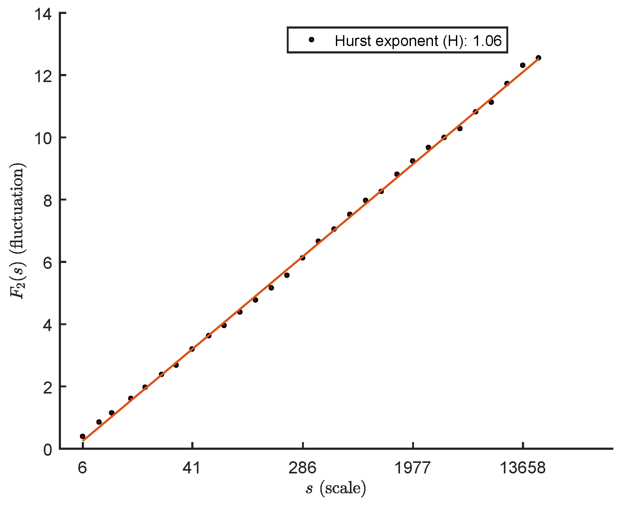
Determine the scaling behavior of the fluctuation function by analyzing the log-log plots $F_q\left(s\right)$ vs. s for each value of q. If the series X is long-range power-law correlated, $F_q\left(s\right)$ will increase, for large values of the timescales s, as power-law, that is:

$$F_q\left(s\right)\sim s^{h\left(q\right)}$$

(7)

For large values of s, the procedure of determining the scaling behavior becomes statistically unreliable because of the number of segments $N_s$ for the averaging procedure in step 4. Hence, it is advised not to overcome the limit $s=N/4$ in the fitting procedure to determine $h\left(q\right)$. For timescale $s\approx 10$, a systematic error can occur even if it can be suitably corrected. The exponent $h\left(q\right)$ may depend on q. The quantity $h\left(q\right)$ is known as the generalized Hurst exponent and for stationary time series $h\left(2\right)$ is identical to the Hurst exponent H [18]. The value of $h\left(0\right)$, which corresponds to the limit of $h\left(q\right)$ for $q\to 0$, cannot be determined directly using the averaging procedure in Equation (6) because of the diverging exponent. Instead, a logarithmic averaging can be employed as:

$$F_q\left(s\right)\equiv \exp {\left\{\frac{1}{4N_s}\sum _{\nu =1}^{2N_s}ln{\left[F^2\left(s,v\right)\right]}^{q/2}\right\}}^{1/q}.$$

(8)

We note that $h\left(0\right)$ cannot be defined for time series with fractal support, where $h\left(q\right)$ diverges for $q\to 0$.

Definition 3

(Multifractal and Monofractal Signals). If the generalized Hurst exponent $h\left(q\right)$ is found independent of q, the time series is monofractal, i.e., it shows a uniform scaling over all magnitude scales of the fluctuations. Conversely, the time series is said to be multifractal when $h\left(q\right)$ depends appreciably on q, so that small fluctuations scale differently from large ones.

It can be shown that the generalized Hurst exponent is related to some classical multifractal indices [41,42]. In particular, $h\left(q\right)$ is directly related to the classical multifractal scaling exponents, also called the Rényi scaling exponent, $\tau \left(q\right)$ by the relation:

$$\tau \left(q\right)=qh\left(q\right)-1,$$

(9)

where $\tau \left(2\right)$ is the correlation dimension. Moreover, the generalized multifractal dimension [43] $D\left(q\right)$ reads as:

$$D\left(q\right)=\frac{\tau \left(q\right)}{q-1}=\frac{qh\left(q\right)-1}{q-1}.$$

(10)

A compact and useful way to express the multifractal characteristic of a time series is the multifractal spectrum $f\left(\tilde{\alpha }\right)$ computed by the Legendre transform of $\tau \left(q\right)$:

$$f\left(\tilde{\alpha }\right)=q\tilde{\alpha }-\tau \left(q\right),$$

(11)

where $\tilde{\alpha }$, called the singularity strength or Hölder exponent, is equal to $\tilde{\alpha }=\frac{d\tau \left(q\right)}{dq}$. Through Equation (9), we find the following relations for the multifractal spectrum:

$$\tilde{\alpha }=h\left(q\right)+q\frac{d\tau \left(q\right)}{dq}\mathrm{and}f\left(\tilde{\alpha }\right)=q[\tilde{\alpha }-h\left(q\right)]+1.$$

(12)

2.2. Data Pre-Processing

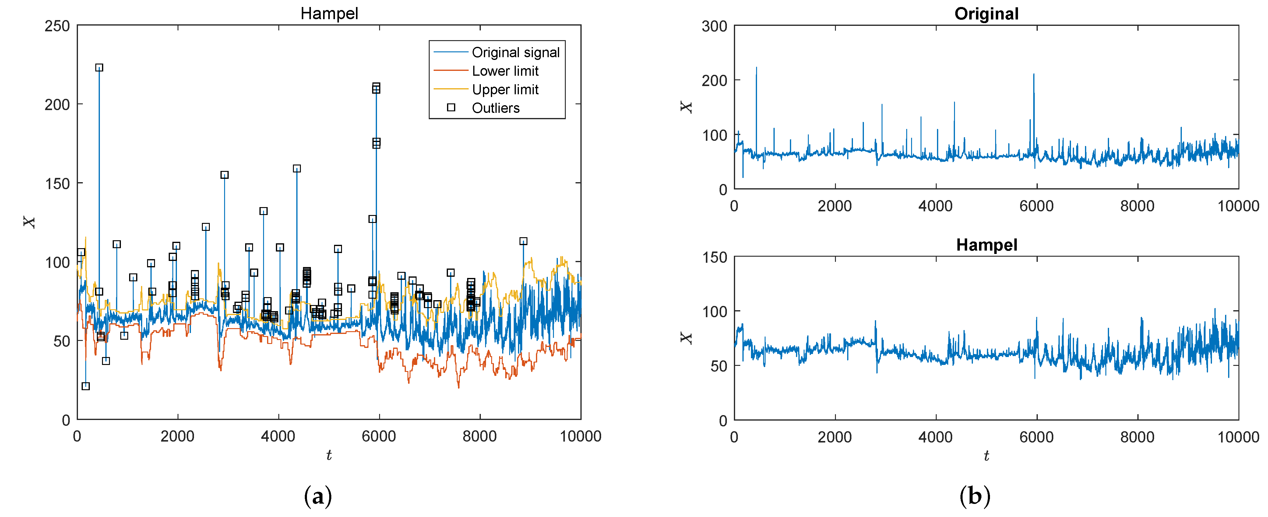
2.2.1. Addressing Outliers

When working with real-world signals, such as signals coming from noisy measuring instruments, a check on the existence of outliers and their removal is of paramount importance before starting any analysis. For the signal under analysis, a simple Hampel filter [44] for outlier detection and substitution is used. It is known that when a dataset contains outliers, even a single out-of-scale observation, the sample mean may deviate significantly [45]. The Hampel filter is based on the fact that a single large observation can make the sample mean and variance cross any bound; thence, a robust estimation of the outlier can be based on the median and the median absolute deviation (MAD) [46].

Given a sequence of values ${\left\{x_k\right\}}_{k=1}^N$ and a sliding window of length k, the local median is defined as:

$$M_i^k=\mathrm{median}(x_{i-k},x_{i-k+1},\dots ,x_i,\dots ,x_{i+k-1},x_{i+k}),$$

(13)

and the standard deviation reads as:

$${\sigma }_i^k=\rho ·\mathrm{median}(x_{i-k},\dots ,x_{i+k}),\mathrm{with}\rho =\frac{1}{\sqrt{2}·{\mathrm{erfc}}^{-1}(1/2)}\approx 1.4826$$

(14)

Finally, the MAD is defined as:

$$\mathrm{MAD}=\frac{{\sigma }_i^k}{\rho }$$

(15)

and, for a given threshold $T_{\sigma }$, the Hampel identifier detects $x_i$ as an outlier and replaces it with $M_i^k$. Even if the Hampel filter treats the process underlying the signal as a sequence of i.i.d. random variables, it is considered extremely effective in practice [47]. Figure 1a shows the detected outliers together with the upper and lower bounds of the signal at hand, while Figure 1b shows the original signal and the processed signal thanks to the Hampel filter.

2.2.2. Filtering out Environmental Factor Outliers

It is essential to filter physiological signals to place them in a suitable frequency band before further analysis [34]. In order to eliminate high frequency noise due to environmental factors, we processed the signal $X\left(t\right)$ with a stable linear-phase low-pass finite impulse response (FIR) filter [48] with the following characteristics. Let $f_N=\frac{f}{f_s/2}\in [0,1]$ be the normalized frequency, where $f_s$ is the sampling frequency (in sample/sec) and $f_s/2$ is the Nyquist frequency; then, the filter design follows:

• Equiripple filter with pass-band frequency: $f_N^{\mathrm{pb}}=0.10$;
• Stop-band frequency: $f_N^{\mathrm{sb}}=0.15$;
• Stop-band attenuation: 60 dB;
• Amplitude of the ripple in the pass-band: 1 dB.

This specific design for the FIR filter yields a computationally light filter whose order is 87. Since the application allows off-line pre-processing, we employ the above filter to run a zero-phase filtering, that is, processing the input signal in both forward and reverse directions. Specifically, after filtering the signal in the forward direction, we reverse the filtered signal and run it back through the filter, yielding zero-phase distortion. In other words, the forward and reverse filtering direction zeroes the measured group delay ${\tau }_g=43.5$ samples. We note that the linear-phase compensation comes with the effect of a filter transfer function which equals the squared magnitude of the original filter transfer function and a filter order that is double of the order of the original filter. Finally, the stop-band frequency $f_N^{\mathrm{sb}}=0.15$ allows the elimination of all frequency components above $f=0.05$ Hz, corresponding to a timescale $t=1/f$ of 5 s.

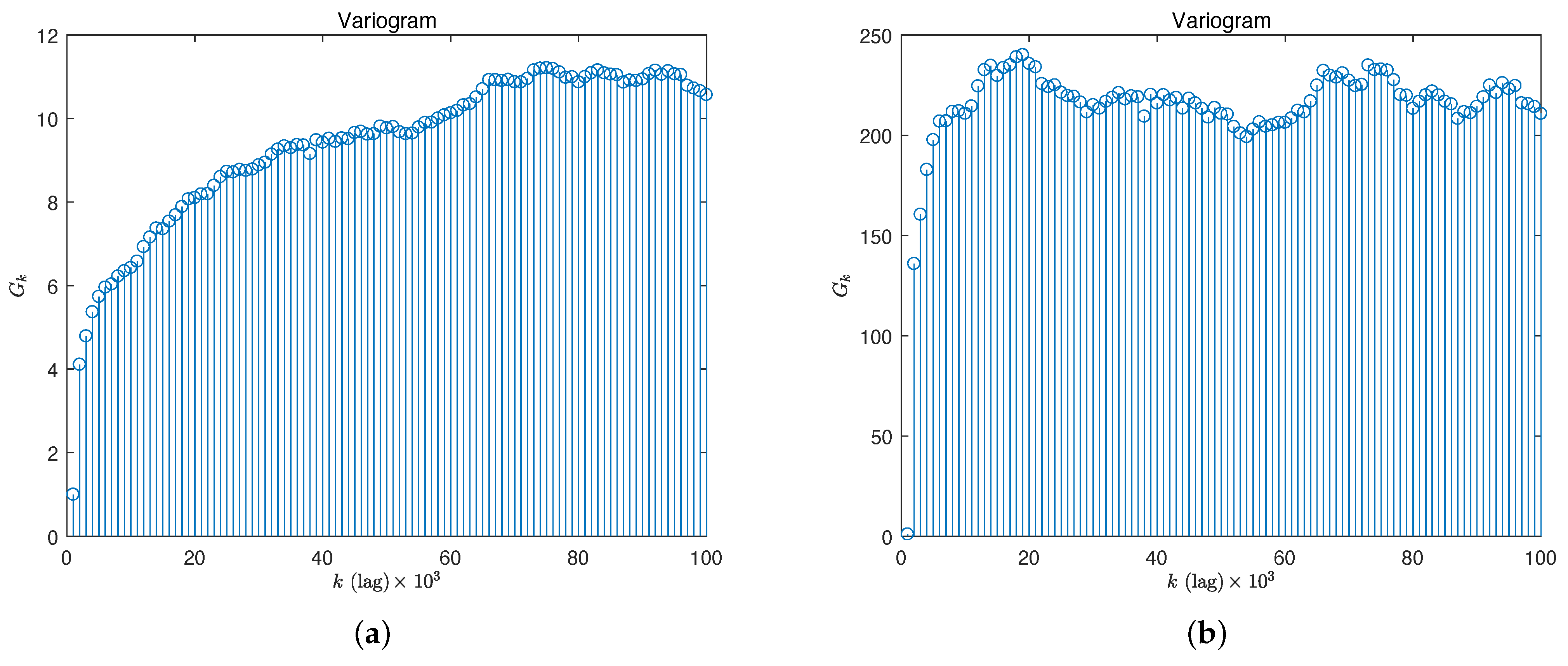
2.2.3. Addressing Non-Stationarities

A random process is said to be stationary if its statistical properties do not change over time. More precisely, for a random process $X\left(t\right)$, the following two definitions hold.

Definition 4

(Strict-Sense Stationary). A random process $X\left(t\right)$ is said to be strict-sense stationary (SSS) if all its finite order distribution are time invariant, i.e., the joint CDF of $X\left(t_1\right),X\left(t_2\right),\dots ,X\left(t_k\right)$ is the same as for $X(t_1+\alpha ),X(t_2+\alpha ),\dots ,X(t_k+\alpha )$ for any k, any $t_1,t_2,\dots ,t_k$, and any timeshift α. Hence, for a SSS process, the first-order distribution is independent of t, and the second-order distribution, i.e., the distribution of any two samples $X\left(t_1\right)$ and $X\left(t_2\right)$, depends only on the distance or lag $\tau =t_1-t_2$.

Definition 5

(Wide-Sense Stationary). A random process $X\left(t\right)$ is said to be wide-sense (or weak-sense) stationary (WSS) if its mean and auto-correlation function are time invariant, i.e., $\mathbb{E}\left(X\right(t\left)\right)=\mu$ and $R_X(t_1,t_2)$ is only a function of the distance or lag $|t_1-t_2|$.

Hence, stationarity refers to time invariance of some, or all, of the statistics of a random process (e.g., mean, auto-correlation, n-th order distribution). It is worth noting that in real-world signals, it is difficult to find a true SSS or WSS signal due to the presence of transient, drift, cycle, polynomial or quasi-periodic trends. However, some random phenomena can exhibit a steady-state behavior after the transient. For example, a random walk is not stationary [49]. DFA is a powerful tool for analyzing the long-range correlations in a real-world signal since it incorporates polynomial detrending routines in its main core, and it has been shown to outperform pre-existing methods, such as $\mathrm{R}-\mathrm{S}$ analysis [50,51], fluctuation analysis [52] or other methods to study the auto-correlation of a signal, such as the decay of the Fourier spectrum [53] or the decay of the auto-correlation function [35]. However, real-world time series such as physiological measurements or even rainfalls and river water flows can be affected by other types of trends such as seasonalities and, more specifically, periodic or quasi-periodic trends [40] that make the signals non-stationary with the appearance of crossovers in the scaling function of the DFA (periodic or quasi-periodic trends). Besides apparent crossovers, a non-stationarity reveals a Hurst exponent $\mathrm{H}>1$ in the DFA scaling function with no clear interpretation in the fractal theory, being for one-dimensional self-affine processes the H exponent related to the fractal dimension $(D=2-\mathrm{H})$ that has to be positive. As an example, in Figure 2, it the log-log plot representing the scaling function $F_2\left(s\right)$ for the BPd signal treated only with outlier removal phase and low-pass filtering can be appreciated. The high value of the Hurst exponent $\mathrm{H}>1$ denotes the presence of non-stationarities not removed by the third order DFA, i.e., DFA3. Notwithstanding, the DFA is able to address polynomial trends—see Section 2.1—and many detrending techniques aiming to study real-world signals are proposed, such as the ones based on empirical mode decomposition, singular value decomposition, Fourier spectrum (Fourier detrended MFDFA), etc.—see [35,54] for further information.

In this work, we concatenate three methods to obtain a near-stationary signal:

• The log transformation, where each sample $X\left(k\right)$ is substituted by $log\left(X\right(k\left)\right)$ [55] in order to stabilize the overall variance of the signal;
• The subtraction from the signal of the overall trend obtained by a median filter with a time window

  $$Y_M\left(k\right)=\left\{\begin{array}{cc}\mathrm{median}\left[X(k-(n-1)/2:k+(n-1)/2)\right]\hfill & \mathrm{if}n\mathrm{is}\mathrm{odd}\hfill \\ \mathrm{median}\left[X(k-n/2,\dots ,k+(n/2)-1)\right]\hfill & \mathrm{if}n\mathrm{is}\mathrm{even}\hfill \end{array}\right.$$

  with $k=4500$ samples;
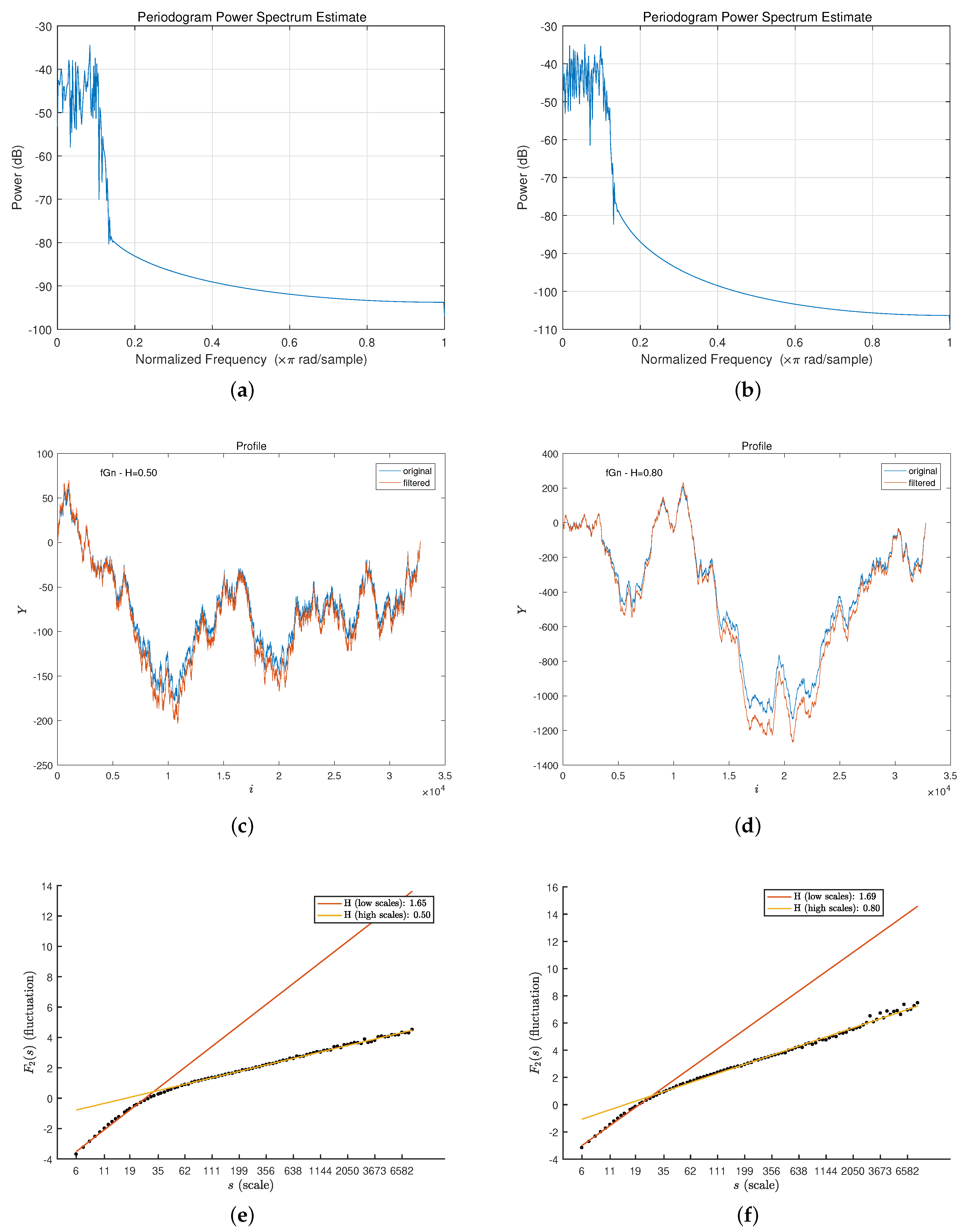
• the so-called Fourier-detrended MFDFA [56], which consists of removing the first $c=60$ sinusoids from the Fourier spectrum, corresponding to slow varying cycles that are sources of residual non-stationarity.

The last detrending method, used in several works in the literature dealing with real-word signals [29,54,57,58], has the drawback of generating an apparent crossover located around the timescales corresponding to the cut-off frequency related to c in the fast Fourier transform (FFT) spectrum [59]. However, this phenomenon is not a real problem here since, as we will see, we are interested in the asymptotic behavior of the scaling function $F_q\left(s\right)$, which is the scaling behavior for higher timescales.

One can experimentally verify the non-stationarity property by computing the variogram $G_k$ that measures the variance of differences k time units apart relative to the variance of the differences 1 time unit apart [60]. Specifically, for a given time series $z_t$, the variogram is defined as:

$$G_k=\frac{\mathrm{Var}(z_{t+k}-z_t)}{\mathrm{Var}(z_{t+1}-z_1)},\mathrm{for}\mathrm{lag}k=1,2,3,\dots$$

(16)

It can be shown that for a stationary process, as k increases, the graph of $G_k$ vs. k approximates to an asymptotic stable behavior, while for a non-stationary process, $G_k$ tends to increase monotonically. In Figure 3a, the variogram for the original signal is reported, while in Figure 3b, the one obtained for the processed signal is shown. The general appearance in Figure 3a does seem to indicate that it does not converge to a stable level, confirming the non-stationary nature of the time series under analysis. Instead, in the processed case, we find a clear plateau indicating the removal of an important amount of non-stationarity. Furthermore, the residual non-stationarity is addressed directly by the MFDFA detrending procedure given a suitable order polynomial.

As noted above, pre-processing of a noisy non-stationary signal can impair the MFDFA analysis due to the appearance of crossovers. As an example, it is well known that the Fourier detrending technique, used to eliminate the low-frequency periodicities, generates a crossover and allows us to measure the multifractal characteristics only after a predefined timescale $s_{\times }$, where the scaling function can be approximated with a linear regression [59]. As expected, the normal low-pass filtering procedure based on a linear-phase FIR filter (whose delay group is suitably compensated) also distorts the scaling function for lower scales. With the aim of understanding the dynamic of such distortion, we generated two synthetic signals of $2^{15}$ samples. One was an uncorrelated signal with a Hurst exponent $\mathrm{H}=0.5$, while the other was a long-range (positively) correlated signal with $\mathrm{H}=0.8$. The correlated fractional Gaussian noise (fGn) was obtained by the FFT algorithm together with an embedding of the covariance matrix in a circulant matrix—see [61,62].

It is worth noting that, for both signals, the scaling function $F_q\left(s\right)$ is a straight line with an angular coefficient equal to H. In Figure 4, the main findings for the synthetic uncorrelated and correlated signals after the FIR filtering are reported. In Figure 4a,b, the power spectrum estimate after the low-pass filtering is reported. Figure 4c,d gives an idea of the profiles of both signals, while Figure 4e,f report the scaling behavior computed by DFA1. In both cases the wide crossovers around $s_{\times }=30$ with a bad Hurst exponent are clearly visible, while the scaling behavior remains the original one for $s_{\times }\gg 30$, that is, for asymptotic timescales. This fact has to be taken into account in analyzing pre-processed real-world signals, such as the one at hand.

3. Results and Discussion

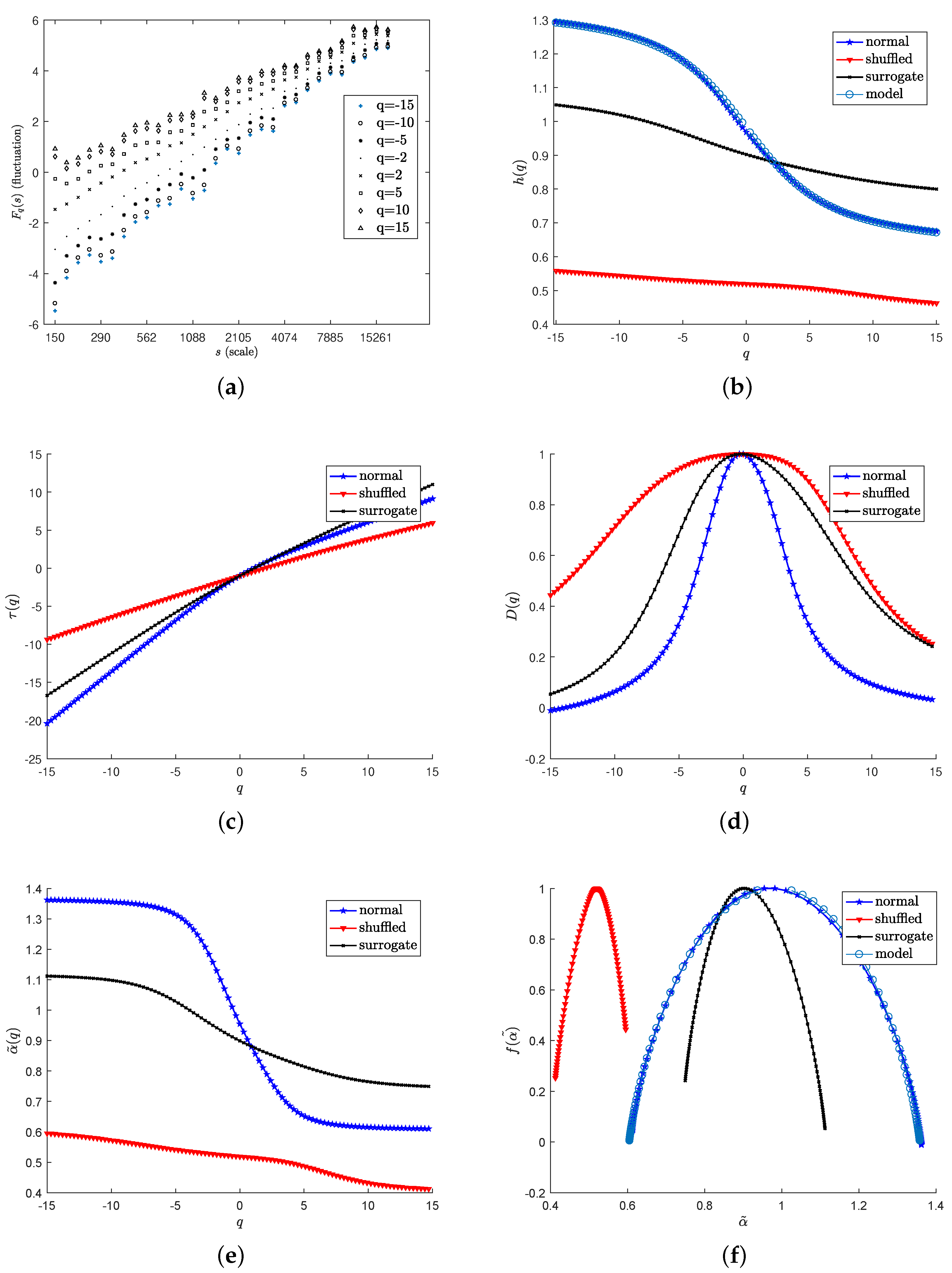
3.1. Multifractal Characterization of the BPd Signal

In describing the multifractal characteristics of the BPd signal at hand we evaluate the DFA3 for timescales higher than $s>150$ until $s=⌊N/5⌋$, where the scaling function $F_q\left(s\right)$ is close to be a straight line for all exponents q and timescales s—see Figure 5a. We report the following main multifractal indices:

• Multifractal strength of the singularity spectrum $f\left(\tilde{\alpha }\right)$:

  $${\Delta }_{\tilde{\alpha }}={\tilde{\alpha }}_{+}-{\tilde{\alpha }}_{-},$$

  (17)

  where ${\tilde{\alpha }}_{+}$, ${\tilde{\alpha }}_{-}$ are the two extreme values at the two ends of the multifractal spectrum support, respectively;
• The asymmetry of the singularity spectrum that is evaluated through a suitable asymmetry index $A_{\tilde{\alpha }}$, that reads as [63]:

  $$A_{\tilde{\alpha }}=\frac{\Delta {\tilde{\alpha }}_L-\Delta {\tilde{\alpha }}_R}{\Delta {\tilde{\alpha }}_L+\Delta {\tilde{\alpha }}_R},$$

  (18)

  with $\Delta {\tilde{\alpha }}_L={\tilde{\alpha }}^{*}-{\tilde{\alpha }}_{-}$ and $\Delta {\tilde{\alpha }}_R={\tilde{\alpha }}_{+}-{\tilde{\alpha }}^{*}$, and where ${\tilde{\alpha }}^{*}$ is the $\tilde{\alpha }$ value at maximum of the singularity spectrum $f\left(\tilde{\alpha }\right)$, i.e., the box counting dimension.

The main results of our investigation are reported in

Table 1. Multifractal indices reported for the BPd signal and estimated parameters of the multiplicative model.

${\tilde{\mathit{\alpha }}}_{+}$	${\tilde{\mathit{\alpha }}}_{-}$	${\tilde{\mathit{\alpha }}}^{*}$	${\mathbf{\Delta }}_{\tilde{\mathit{\alpha }}}$	${\mathit{A}}_{\tilde{\mathit{\alpha }}}$	$\mathit{h}\left(2\right)$	$\mathit{\tau }\left(2\right)$	a	b
1.362	0.610	0.997	0.752	0.011	0.880	0.850	$0.6576\pm 0.0014$	$0.39\pm 0.0008$

. In particular, the shape parameters of the multifractal spectrum are provided, such as ${\tilde{\alpha }}_{-}$, ${\tilde{\alpha }}_{+}$, ${\tilde{\alpha }}^{*}$, ${\Delta }_{\tilde{\alpha }}$ and $A_{\tilde{\alpha }}$, together with the Hurst exponent $\mathrm{H}=h\left(2\right)$ and the correlation dimension $\tau \left(2\right)$. As concerns the multifractal strength, we find a higher value ${\Delta }_{\tilde{\alpha }}=0.752$ and a symmetric spectrum, with a small $A_{\tilde{\alpha }}=0.011$, that together with the correlation dimension $\tau \left(2\right)$ indicate a strong multifractality of the BPd signal. Finally, the Hurst exponent $\mathrm{H}=0.880$ indicates the presence of long-range correlations.

As concerns the multifractal nature, it is possible to distinguish from multifractality due to the wideness of the PDF [64] and multifractality due to the two different correlations in small- and large-scale fluctuations. These two kinds of multifractality can be assessed by evaluating two time series derived from the original one: the shuffled time series and the surrogate one. The former is computed by simply shuffling at random the time indices, while the latter is obtained by changing the phases, computed through the discrete Fourier transform (DFT) of the original signal, drawing from a uniform distribution in $(-\pi ,\pi )$ [65]. In the last case, one can demonstrate that the PDF tends to be normally distributed but correlations do not change, destroying intrinsic non-linearity. The shuffling procedure will destroy all long-range correlations and the corresponding shuffled time series will exhibit monofractal scaling. Conversely, the multifractality due to the wideness of the PDF is not affected by the shuffling procedure. Since the shuffling of time series destroys the long-range correlations, if the multifractality is due only to long-range correlations, then one should expect a constant value $h_{\mathrm{shuffle}}=0.5$. If both types of multifractality are present, the shuffled and the surrogate series will show weaker multifractality with respect to the original series.

In order to give a complete picture of the multifractal characteristics of the analyzed BPd time series, in Figure 5 and its respective panels, the main multifractal diagrams obtained from the MFDFA and the application of the whole multifractal analysis procedure are reported. Panel (a) reports the scaling function $F_q\left(s\right)$ vs. s for the MFDFA3 parametrized with the moment values $q\in \left\{-15,-10,-5,-2,2,5,10,15\right\}$. The BPd signal scales differently depending on q for a wide range of timescales s after $s_{\times }=150$, indicating the presence of multifractality. Panel (b) shows how the generalized Hurst exponent $h\left(q\right)$ is a non-linear decreasing function of q that, together with the non-linear behavior of the mass exponent $\tau \left(q\right)$ vs. q—panel (c)—the Hölder exponent $\tilde{\alpha }\left(q\right)$ vs. q—panel (e)—and the amplitude of the singularity spectrum $f\left(\tilde{\alpha }\right)$—panel (f)—demonstrate the multifractality of the BPd time series. In particular, from panel (b), by considering the diagram for the shuffled series, we can see that the shuffling procedure actually destroys all long-range correlations in the original signal (indicated as “normal” in the plot) with $h_{\mathrm{shuffle}}\left(2\right)$ being nearly linear, and $h\left(2\right)$ close to the value for an uncorrelated signal. Therefore, it is possible to conclude that the long-range correlations do not depend on the wideness of the PDF of the signal: rather, they are an intrinsic feature of the complexity of the signal under analysis. Finally, the surrogate series, with $h\left(2\right)\approx h_{\mathrm{surr}}\left(2\right)$, shows that the long-range correlations in the “monofractal zone”, described by the exponent $h\left(2\right)$, are not destroyed, while the intrinsic non-linearity are eliminated.

3.2. Fitting a Multiplicative Cascade Model

As a last task, we investigate the possibility of describing the multifractal dynamic with a concise multiplicative model. We find that a particular multifractal model, originally proposed in the geophysical field [38,39], to model rainfall and river flows, fits well with the time series under analysis. Specifically, the statistical properties of the BPd signal are very similar to the ones pertaining to the class of the multiplicative cascade models [36,66]. In panels (b,f) of Figure 5, the fitted curves represented as circles for $h\left(q\right)$ and $f\left(\tilde{\alpha }\right)$ show that in the whole q-range, i.e., $q\in \left[-15,15\right]$, the exponents can be well-approximated by the formula [38]:

$$h\left(q\right)=\frac{1}{q}-\frac{ln(a^q+b^q)}{qln\left(2\right)},$$

(19)

with $ln\left(x\right)$ being the natural logarithm of x. Equation (19) is derived from a modification of the (non-conservative) multiplicative multifractal cascade model—see Appendix A—with two masses. The advantage of this model is that it can be suitably described by only two parameters, namely a and b. The fitting results are $a=0.6576\pm 0.0014$ and $b=0.39\pm 0.0008$, with a fitting total sum-of-squares error equal to 0.0023.

4. Conclusions

In this paper, the multi-fractal properties of a human body diastolic blood pressure has been investigated in a time span of circa one day within a given frequency spectrum for asymptotic timescales. The signal shows nice scaling properties and long-range correlations. Moreover, the moments are found to scale differently in a wide range of timescales, indicating the presence of multifractality. The shuffles and surrogate tests demonstrate the nature of multifractality that is found in the long-range correlations and intrinsic non-linearity. Hence, a modified binomial multiplicative model is fitted showing how the signal at hand can be described concisely with a multiplicative model with only two parameters.

In our future research agenda, we plan to use the multifractal indices and the parameters of the multiplicative model as candidate features to train machine learning models for unsupervised or supervised learning (e.g., to discriminate patients according to their physiological signals).

References

1. Nie, C.Y.; Sun, H.X.; Wang, J. The Relationship between Chaotic Characteristics of Physiological Signals and Emotion Based on Approximate Entropy. In Proceedings of the 2nd International Conference on Computer Science and Electronics Engineering (ICCSEE 2013), Hangzhou, China, 22–23 March 2013; Atlantis Press: New York, NY, USA, 2013; pp. 552–555. [Google Scholar] [CrossRef]
2. Ihlen, E. Introduction to Multifractal Detrended Fluctuation Analysis in Matlab. Front. Physiol. 2012, 3, 141. [Google Scholar] [CrossRef] [PubMed]
3. Naraei, P.; Abhari, A.; Sadeghian, A. Application of multilayer perceptron neural networks and support vector machines in classification of healthcare data. In Proceedings of the 2016 Future Technologies Conference (FTC), San Francisco, CA, USA, 6–7 December 2016; pp. 848–852. [Google Scholar] [CrossRef]
4. Naraei, P.; Sadeghian, A. A PCA based feature reduction in intracranial hypertension analysis. In Proceedings of the 2017 IEEE 30th Canadian Conference on Electrical and Computer Engineering (CCECE), Windsor, ON, Canada, 30 April–3 May 2017; pp. 1–6. [Google Scholar] [CrossRef]
5. Naraei, P.; Nouri, M.; Sadeghian, A. Toward learning intracranial hypertension through physiological features: A statistical and machine learning approach. In Proceedings of the 2017 Intelligent Systems Conference (IntelliSys), London, UK, 7–8 September 2017; pp. 395–399. [Google Scholar] [CrossRef]
6. Glass, L. Synchronization and rhythmic processes in physiology. Nature 2001, 410, 277–284. [Google Scholar] [CrossRef]
7. Peng, C.K.; Mietus, J.; Hausdorff, J.M.; Havlin, S.; Stanley, H.E.; Goldberger, A.L. Long-range anticorrelations and non-Gaussian behavior of the heartbeat. Phys. Rev. Lett. 1993, 70, 1343–1346. [Google Scholar] [CrossRef] [PubMed]
8. Kobayashi, M.; Musha, T. 1/f Fluctuation of Heartbeat Period. IEEE Trans. Biomed. Eng. 1982, BME-29, 456–457. [Google Scholar] [CrossRef]
9. Ivanov, P.C.; Amaral, L.A.N.; Goldberger, A.L.; Havlin, S.; Rosenblum, M.G.; Struzik, Z.R.; Stanley, H.E. Multifractality in human heartbeat dynamics. Nature 1999, 399, 461–465. [Google Scholar] [CrossRef]
10. Turcott, R.G.; Teich, M.C. Fractal character of the electrocardiogram: Distinguishing heart-failure and normal patients. Ann. Biomed. Eng. 1996, 24, 269–293. [Google Scholar] [CrossRef]
11. Roach, D.; Sheldon, A.; Wilson, W.; Sheldon, R. Temporally localized contributions to measures of large-scale heart rate variability. Am. J. Physiol.-Heart Circ. Physiol. 1998, 274, H1465–H1471. [Google Scholar] [CrossRef] [PubMed]
12. Wagner, C.; Nafz, B.; Persson, P. Chaos in blood pressure control. Cardiovasc. Res. 1996, 31, 380–387. [Google Scholar] [CrossRef]
13. Marsh, D.J.; Osborn, J.L.; Cowley, A.W. 1/f fluctuations in arterial pressure and regulation of renal blood flow in dogs. Am. J. Physiol.-Ren. Physiol. 1990, 258, F1394–F1400. [Google Scholar] [CrossRef]
14. Wagner, C.D.; Persson, P.B. Two ranges in blood pressure power spectrum with different 1/f characteristics. Am. J. Physiol.-Heart Circ. Physiol. 1994, 267, H449–H454. [Google Scholar] [CrossRef]
15. Piper, I.; Citerio, G.; Chambers, I.; Contant, C.; Enblad, P.; Fiddes, H.; Howells, T.; Kiening, K.; Nilsson, P.; Yau, Y.H. The BrainIT group: Concept and core dataset definition. Acta Neurochir. 2003, 145, 615–629. [Google Scholar] [CrossRef]
16. Jain, V.; Choudhary, J.; Pandit, R. Blood Pressure Target in Acute Brain Injury. Indian J. Crit. Care Med. Indian Soc. Crit. Care Med. 2019, 23, S136–S139. [Google Scholar] [CrossRef] [PubMed]
17. Peng, C.K.; Buldyrev, S.V.; Havlin, S.; Simons, M.; Stanley, H.E.; Goldberger, A.L. Mosaic organization of DNA nucleotides. Phys. Rev. E 1994, 49, 1685–1689. [Google Scholar] [CrossRef] [PubMed]
18. Kantelhardt, J.W.; Zschiegner, S.A.; Koscielny-Bunde, E.; Havlin, S.; Bunde, A.; Stanley, H.E. Multifractal detrended fluctuation analysis of nonstationary time series. Phys. A Stat. Mech. Its Appl. 2002, 316, 87–114. [Google Scholar] [CrossRef]
19. Buldyrev, S.V.; Goldberger, A.L.; Havlin, S.; Mantegna, R.N.; Matsa, M.E.; Peng, C.K.; Simons, M.; Stanley, H.E. Long-range correlation properties of coding and noncoding DNA sequences: GenBank analysis. Phys. Rev. E 1995, 51, 5084–5091. [Google Scholar] [CrossRef]
20. Bunde, A.; Havlin, S.; Kantelhardt, J.W.; Penzel, T.; Peter, J.H.; Voigt, K. Correlated and Uncorrelated Regions in Heart-Rate Fluctuations during Sleep. Phys. Rev. Lett. 2000, 85, 3736–3739. [Google Scholar] [CrossRef]
21. Moret, M.A.; Zebende, G.F.; Nogueira, E.; Pereira, M.G. Fluctuation analysis of stellar x-ray binary systems. Phys. Rev. E 2003, 68, 041104. [Google Scholar] [CrossRef]
22. Bai, M.Y.; Zhu, H.B. Power law and multiscaling properties of the Chinese stock market. Phys. A Stat. Mech. Its Appl. 2010, 389, 1883–1890. [Google Scholar] [CrossRef]
23. Alvarez-Ramirez, J.; Rodriguez, E.; Echeverria, J.C. A DFA approach for assessing asymmetric correlations. Phys. A Stat. Mech. Its Appl. 2009, 388, 2263–2270. [Google Scholar] [CrossRef]
24. Lévy-Véhel, J.; Lutton, E.; Tricot, C. Fractals in Engineering, 1st ed.; Springer: Berlin, Gemrnay, 2005. [Google Scholar]
25. Aggarwal, S.K.; Lovallo, M.; Khan, P.K.; Rastogi, B.K.; Telesca, L. Multifractal detrended fluctuation analysis of magnitude series of seismicity of Kachchh region, Western India. Phys. A Stat. Mech. Its Appl. 2015, 426, 56–62. [Google Scholar] [CrossRef]
26. Mali, P.; Mukhopadhyay, A. Multifractal characterization of gold market: A multifractal detrended fluctuation analysis. Phys. A Stat. Mech. Its Appl. 2014, 413, 361–372. [Google Scholar] [CrossRef]
27. Telesca, L.; Lovallo, M.; Kanevski, M. Power spectrum and multifractal detrended fluctuation analysis of high-frequency wind measurements in mountainous regions. Appl. Energy 2016, 162, 1052–1061. [Google Scholar] [CrossRef]
28. Mali, P.; Sarkar, S.; Ghosh, S.; Mukhopadhyay, A.; Singh, G. Multifractal detrended fluctuation analysis of particle density fluctuations in high-energy nuclear collisions. Phys. A Stat. Mech. Its Appl. 2015, 424, 25–33. [Google Scholar] [CrossRef]
29. Wang, F.; Liao, G.p.; Li, J.h.; Li, X.c.; Zhou, T.j. Multifractal detrended fluctuation analysis for clustering structures of electricity price periods. Phys. A Stat. Mech. Its Appl. 2013, 392, 5723–5734. [Google Scholar] [CrossRef]
30. De Santis, E.; Sadeghian, A.; Rizzi, A. A smoothing technique for the multifractal analysis of a medium voltage feeders electric current. Int. J. Bifurc. Chaos 2017, 27, 1750211. [Google Scholar] [CrossRef]
31. Thomas, R.; Hsi, L.L.; Boon, S.C.; Gunawan, E. Classification of severity of mitral regurgitation patients using multifractal analysis. In Proceedings of the 2016 38th Annual International Conference of the IEEE Engineering in Medicine and Biology Society (EMBC), Orlando, FL, USA, 16–20 August 2016; pp. 6226–6229. [Google Scholar] [CrossRef]
32. Livi, L.; Maiorino, E.; Rizzi, A.; Sadeghian, A. On the long-term correlations and multifractal properties of electric arc furnace time series. Int. J. Bifurc. Chaos 2016, 26, 1650007. [Google Scholar] [CrossRef]
33. Kimiagar, S.; Movahed, M.S.; Khorram, S.; Sobhanian, S.; Tabar, M.R.R. Fractal analysis of discharge current fluctuations. J. Stat. Mech. Theory Exp. 2009, 2009, P03020. [Google Scholar] [CrossRef]
34. Burr, R.L.; Kirkness, C.J.; Mitchell, P.H. Detrended fluctuation analysis of intracranial pressure predicts outcome following traumatic brain injury. IEEE Trans. Biomed. Eng. 2008, 55, 2509–2518. [Google Scholar] [CrossRef]
35. Kantelhardt, J.W. Fractal and Multifractal Time Series. In Mathematics of Complexity and Dynamical Systems; Meyers, R.A., Ed.; Springer: New York, NY, USA, 2012; pp. 463–487. [Google Scholar] [CrossRef]
36. Feder, J. Fractals, 1st ed.; Springer Science & Business Media: New York, NY, USA, 2013. [Google Scholar]
37. Meneveau, C.; Sreenivasan, K. The multifractal spectrum of the dissipation field in turbulent flows. Nucl. Phys. B Proc. Suppl. 1987, 2, 49–76. [Google Scholar] [CrossRef]
38. Koscielny-Bunde, E.; Kantelhardt, J.W.; Braun, P.; Bunde, A.; Havlin, S. Long-term persistence and multifractality of river runoff records: Detrended fluctuation studies. J. Hydrol. 2006, 322, 120–137. [Google Scholar] [CrossRef]
39. Kantelhardt, J.W.; Koscielny-Bunde, E.; Rybski, D.; Braun, P.; Bunde, A.; Havlin, S. Long-term persistence and multifractality of precipitation and river runoff records. J. Geophys. Res. Atmos. 2006, 111. [Google Scholar] [CrossRef]
40. Hu, K.; Ivanov, P.C.; Chen, Z.; Carpena, P.; Stanley, H.E. Effect of trends on detrended fluctuation analysis. Phys. Rev. E 2001, 64, 011114. [Google Scholar] [CrossRef] [PubMed]
41. Yu, Z.; Yee, L.; Zu-Guo, Y. Relationships of exponents in multifractal detrended fluctuation analysis and conventional multifractal analysis. Chin. Phys. B 2011, 20, 090507. [Google Scholar]
42. Shang, P.; Lu, Y.; Kamae, S. Detecting long-range correlations of traffic time series with multifractal detrended fluctuation analysis. Chaosb Solitons Fractals 2008, 36, 82–90. [Google Scholar] [CrossRef]
43. Harte, D. Multifractals: Theory and Applications; Chapman & Hall/CRC: New York, NY, USA, 2001. [Google Scholar]
44. Hampel, F.R. A general qualitative definition of robustness. Ann. Math. Stat. 1971, 42, 1887–1896. [Google Scholar] [CrossRef]
45. Liu, H.; Shah, S.; Jiang, W. On-line outlier detection and data cleaning. Comput. Chem. Eng. 2004, 28, 1635–1647. [Google Scholar] [CrossRef]
46. Leys, C.; Ley, C.; Klein, O.; Bernard, P.; Licata, L. Detecting outliers: Do not use standard deviation around the mean, use absolute deviation around the median. J. Exp. Soc. Psychol. 2013, 49, 764–766. [Google Scholar] [CrossRef]
47. Pearson, R.K. Outliers in process modeling and identification. IEEE Trans. Control. Syst. Technol. 2002, 10, 55–63. [Google Scholar] [CrossRef]
48. Oppenheim, A.V.; Schafer, R.W. Discrete-Time Signal Processing, 3rd ed.; Pearson Higher Education: London, UK, 2010. [Google Scholar]
49. Howard, R.M. A Signal Theoretic Introduction to Random Processes; John Wiley & Sons: New York, NY, USA, 2015. [Google Scholar]
50. Hurst, H.E. Long-term storage capacity of reservoirs. Trans. Am. Soc. Civil Eng. 1951, 116, 770–808. [Google Scholar] [CrossRef]
51. Mandelbrot, B.B.; Van Ness, J.W. Fractional Brownian motions, fractional noises and applications. SIAM Rev. 1968, 10, 422–437. [Google Scholar] [CrossRef]
52. Bunde, A.; Havlin, S. Fractals in Science; Springer: Berlin, Germany, 2013. [Google Scholar]
53. Hunt, G. Random fourier transforms. Trans. Am. Math. Soc. 1951, 71, 38–69. [Google Scholar] [CrossRef]
54. Bashan, A.; Bartsch, R.; Kantelhardt, J.W.; Havlin, S. Comparison of detrending methods for fluctuation analysis. Phys. A Stat. Mech. Its Appl. 2008, 387, 5080–5090. [Google Scholar] [CrossRef]
55. Lütkepohl, H.; Xu, F. The role of the log transformation in forecasting economic variables. Empir. Econ. 2012, 42, 619–638. [Google Scholar] [CrossRef]
56. Chianca, C.; Ticona, A.; Penna, T. Fourier-detrended fluctuation analysis. Phys. A Stat. Mech. Its Appl. 2005, 357, 447–454. [Google Scholar] [CrossRef]
57. Zhao, X.; Shang, P.; Lin, A.; Chen, G. Multifractal Fourier detrended cross-correlation analysis of traffic signals. Phys. A Stat. Mech. Its Appl. 2011, 390, 3670–3678. [Google Scholar] [CrossRef]
58. Movahed, M.S.; Jafari, G.; Ghasemi, F.; Rahvar, S.; Tabar, M.R.R. Multifractal detrended fluctuation analysis of sunspot time series. J. Stat. Mech. Theory Exp. 2006, 2006, P02003. [Google Scholar] [CrossRef]
59. Hu, J.; Gao, J.; Wang, X. Multifractal analysis of sunspot time series: The effects of the 11-year cycle and Fourier truncation. J. Stat. Mech. Theory Exp. 2009, 2009, P02066. [Google Scholar] [CrossRef]
60. Bisgaard, S.; Kulahci, M. Time Series Analysis and Forecasting by Example; John Wiley & Sons: New York, NY, USA, 2011. [Google Scholar]
61. Beran, J. Statistics for Long-Memory Processes; CRC Press: New York, NY, USA, 1994; Volume 61. [Google Scholar]
62. Davies, R.B.; Harte, D. Tests for Hurst effect. Biometrika 1987, 74, 95–101. [Google Scholar] [CrossRef]
63. Drożdż, S.; Oświȩcimka, P. Detecting and interpreting distortions in hierarchical organization of complex time series. Phys. Rev. E 2015, 91, 030902. [Google Scholar] [CrossRef]
64. Mandelbrot, B.B.; Wallis, J.R. Some long-run properties of geophysical records. Water Resour. Res. 1969, 5, 321–340. [Google Scholar] [CrossRef]
65. Schreiber, T.; Schmitz, A. Surrogate time series. Phys. D Nonlinear Phenom. 2000, 142, 346–382. [Google Scholar] [CrossRef]
66. Barabási, A.L.; Vicsek, T. Multifractality of self-affine fractals. Phys. Rev. A 1991, 44, 2730–2733. [Google Scholar] [CrossRef] [PubMed]
Figure 1. Results of the Hampel filtering procedure for outlier removals (a). Original time series (top panel) and processed time series (bottom panel) (b). In the last panel the presence of a high non-stationary behavior, such as slow varying cycles, can be observed that needs to be addressed before operating the MFDFA. The bottom panel in (b) also shows a set of singularities for the processed signal, such as cuspids and stairs.
Algorithms 15 00259 g001
Figure 2. Scaling function F 2 ( s ) computed through the DFA3 for the BPd signal filtered with the Hampel and the low-pass FIR filters, but not pre-treated for addressing non-stationarity.
Algorithms 15 00259 g002
Figure 3. Variogram for the original time series (a) and after the non-stationarity removal (b).
Algorithms 15 00259 g003
Figure 4. The behavior of the DFA1 scaling function F 2 ( s ) for two synthetic signals with Hurst exponent H = 0.5 (uncorrelated) and H = 0.8 (positively correlated) for a wide timescale range s. Panels (a,b) depict the power spectral density for both signals, showing how the linear-phase FIR filter suppresses the frequency components after a given cut-off frequency. Panels (c,d) report the profile Y ( i ) of both signals for the original and filtered version. Finally, panels (e,f) show the appearance of a crossover placed at low timescales due to the filtering process for both filtered signals in the DFA1 plot. However, the correct scaling behavior is asymptotically restored, i.e., it remains unchanged for higher timescale values.
Algorithms 15 00259 g004
Figure 5. Results of the MFDFA3 on the BPd signal. Panel (a) reports the F q ( s ) vs. s diagram varying the timescale s in a wide range of values. Results of the MFDFA3 on the BPd signal for the original (normal), shuffled and surrogate time series. Panel (b) shows the h ( q ) vs. q diagram. Circles denotes the modified multiplicative model fitted to the data. Panels (ce) report the mass exponent τ ( q ) vs. q, the generalized dimension D ( q ) vs. q and the Hölder exponent α ˜ ( q ) vs. q diagrams derived from the multifractal formalism. Panel (f) shows the multifractal spectrum for the BPd signal. The high amplitude Δ α ˜ of the multifractal spectrum together with the non-linear behavior of h ( q ) and τ ( q ) demonstrate a strong multifractal signature of the analyzed signal. Shuffled and surrogate series indicate that the multifractality is due to long-range correlations. Finally, the near-optimal fitting of the modified multiplicative cascade model (A3), represented as circles in panels (b), shows that the BPd signal can be described concisely by only two parameters a and b.
Algorithms 15 00259 g005