Research of Flexible Assembly of Miniature Circuit Breakers Based on Robot Trajectory Optimization

Abstract

This paper is dedicated to achieving flexible automatic assembly of miniature circuit breakers (MCBs) to resolve the high rigidity issue of existing MCB assembly by proposing a flexible automatic assembly process and method with industrial robots. To optimize the working performance of the robot, a time-optimal trajectory planning method of the improved Particle Swarm Optimization (PSO) with a multi-optimization mechanism is proposed. The solution uses a fitness switch function for particle sifting to improve the stability of the acceleration and jerk of the robot motion as well as to increase the computational efficiency. The experimental results show that the proposed method achieves flexible assembly for multi-type MCB parts of varying postures. Compared with other optimization algorithms, the proposed improved PSO is significantly superior in both computational efficiency and optimization accuracy. Compared with the standard PSO, the proposed trajectory planning method shortens the assembly time by 6.9 s and raises the assembly efficiency by 16.7%. The improved PSO is implemented on the experimental assembly platform and achieves smooth and stable operations, which proves the high significance and practicality for MCB fabrication.

1. Introduction

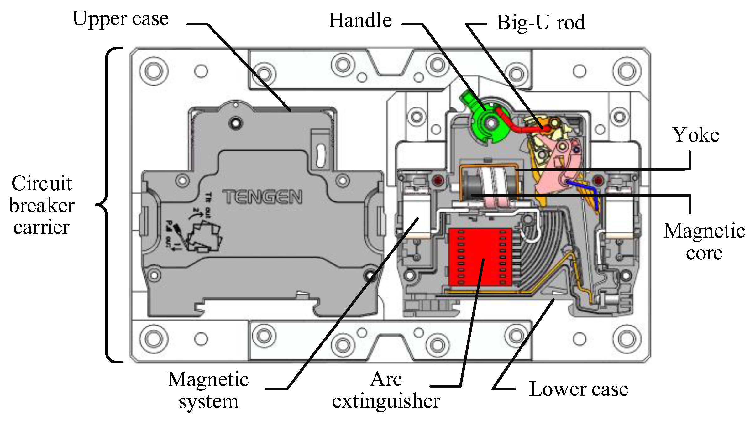
Miniature circuit breakers (MCBs) are important electrical devices in power distribution networks to provide fault current protection, and have been widely used in industrial applications [1,2]. Most MCB parts are in irregular shapes, and it is usually difficult to implement the automatic assembly via machine. The existing MCB assembly techniques are mostly high-rigidity approaches that separately adjust and assemble different MCB parts by a number of specific devices, which are expensive and inflexible. It is eagerly expected that researchers can propose an automatic assembly scheme with industrial robots which are widely applied in manufacturing industries [3,4], to improve the flexibility and efficiency of MCB manufacturing. The key technology of flexible MCB assembly is to adjust randomly postured MCB parts to pre-defined postures with a single robot, so that then the parts can be correctly and accurately assembled. Hence, it is of great significance for improving the production efficiency as well as reducing the production cost.

In practice, the working performance is largely dependent on the robot trajectory. The trajectory planning is a fundamental problem discussed for robot applications [5,6,7]. It is a nonlinear, multi-coupling, multi-constraint multi-objective optimization problem that aims to find the optimal trajectory of the robot based on the corresponding algorithm and boundary constraints under the condition of a given task point [8,9,10]. Existing optimal trajectory planning methods can be divided into four categories by the objective function: 1. minimum time; 2. optimal trajectory smoothness and minimum jerk; 3. minimum energy [11]; 4. hybrid criteria of the conditions above [12].

In terms of time-based optimal trajectory planning, there is a contradiction between time and motion stability. Motion acceleration is achieved by rapid changes of the velocity and acceleration, which leads to a large shock load. For the realization of robot time optimal trajectory planning, the current research mainly focuses on polynomial trajectory interpolation and trajectory algorithm optimization. Huang et al. [13] proposed cubic B-spline curve method to construct parametric paths. Kim et al. [14] proposed a cubic polynomial method that takes the joint position and speed as the constraints, plans the trajectory offline, and then tracks the trajectory online in real-time. The method is easy to be applied, but does not consider the constraints such as the torque and acceleration of the joints, which causes strong shocks and sudden acceleration changes. Ma et al. [15] proposed a sixth-degree polynomial method that solves the discontinuity of the segmental interpolation by low-degree polynomials in the motion process, and prevents problems such as sudden acceleration changes and operating shocks of the manipulator. However, a high polynomial degree causes high computational complexity as well as the oscillation of the interpolation (called the "Runge" phenomenon) [16]. Guan et al. [17,18] propose a method employing the NURBS curve which is characterized by derivative continuity, effective segmentation and strong local support, but it is also computationally complex when solving complex robot paths. Artificial intelligence algorithms are applied for trajectory optimization. Huang et al. [19] use the elitist non-dominated sorting genetic algorithm to optimize robot traveling time and mean jerk. Ajayi et al. [20] seek to obtain the optimal time via the Genetic Algorithm (GA) which is of low computational requirements and high versatility, as well as the reduction of optimization objectives and constraints. PSO has advantages in optimization range, robustness, and scalability. Yan et al. [21] use the standard Particle Swarm Optimization (PSO) algorithm to study the axis trajectory planning for flank milling with conical tools. Yang et al. [22] proposed a PSO method enhanced by an improved annealing schedule, to explore for more candidate solutions and increase the probability of finding the global optima. Shen et al. [23] proposed a UAV path planning method that introduced a Tabu table into particle swarm optimization (PSO) to improve its optimization ability, and obtained the initial detection route of UAVs based on a “minimum ring” method. Shi et al. [24] applied the golden section method is used to find the maximum of velocity, acceleration, and jerk, and utilized a PSO with variable learning factors for global optima searching. PSO realizes the dynamic trajectory optimization by its high ergodicity and time interval adaptivity. However, with the increase of the optimization space, the algorithm performance and accuracy decline with the increasing of the optimization space.

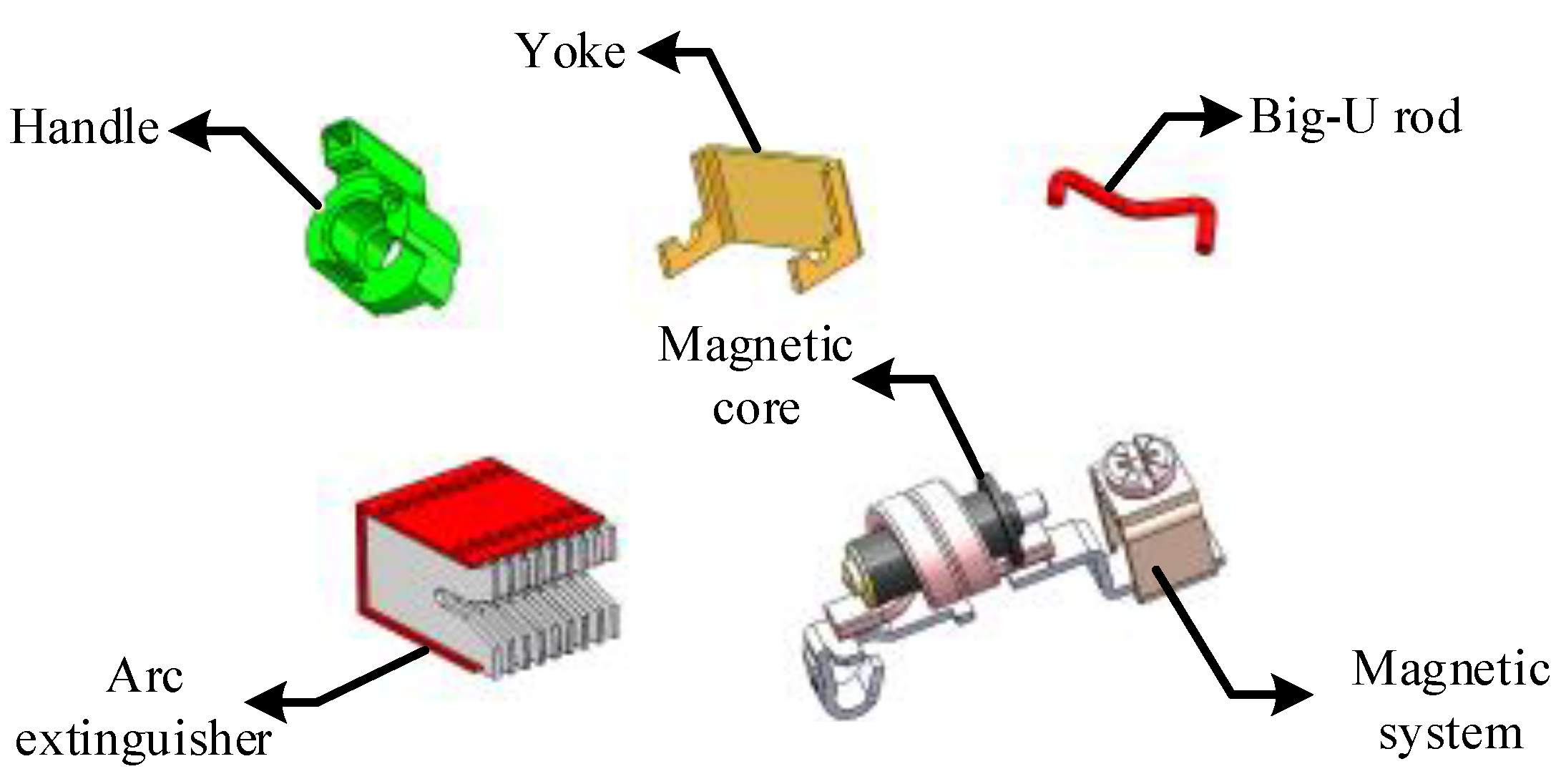
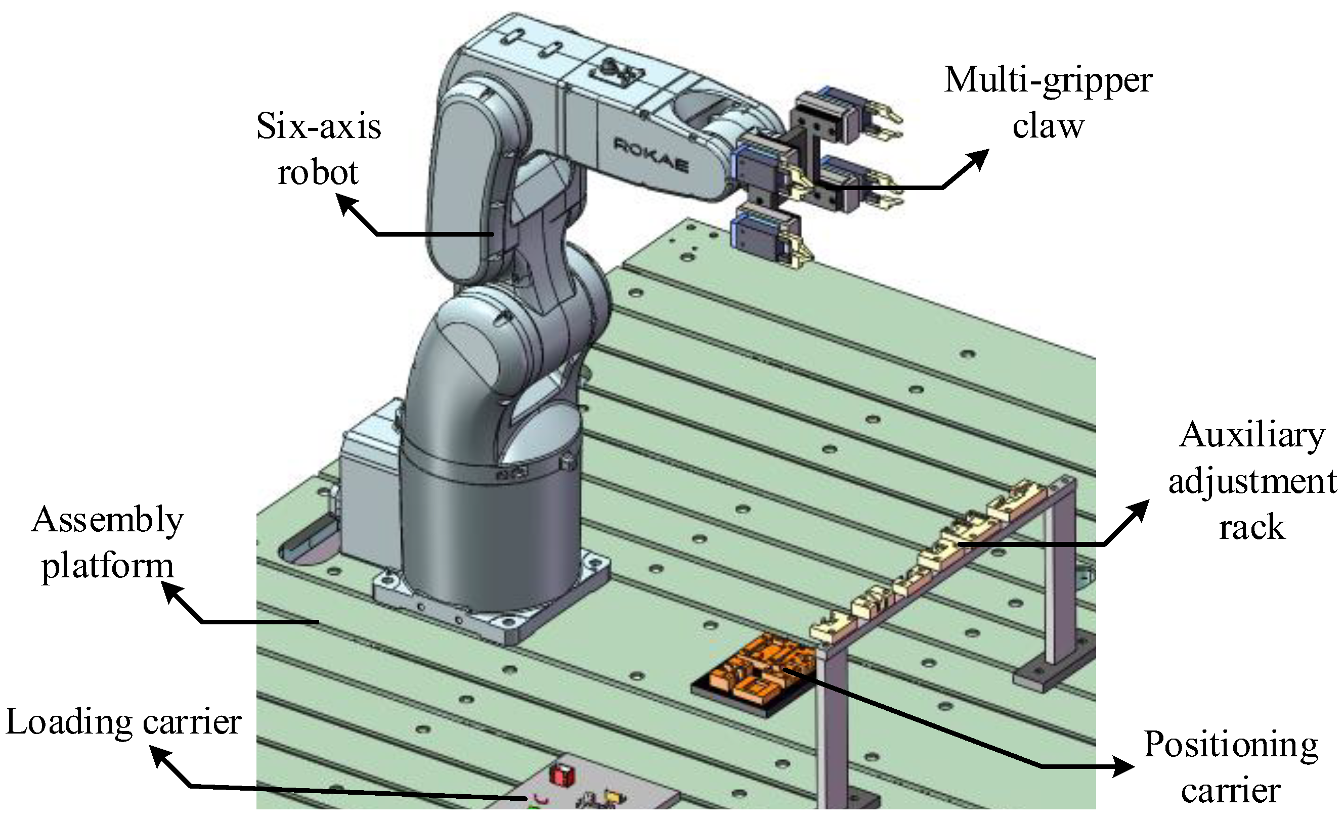
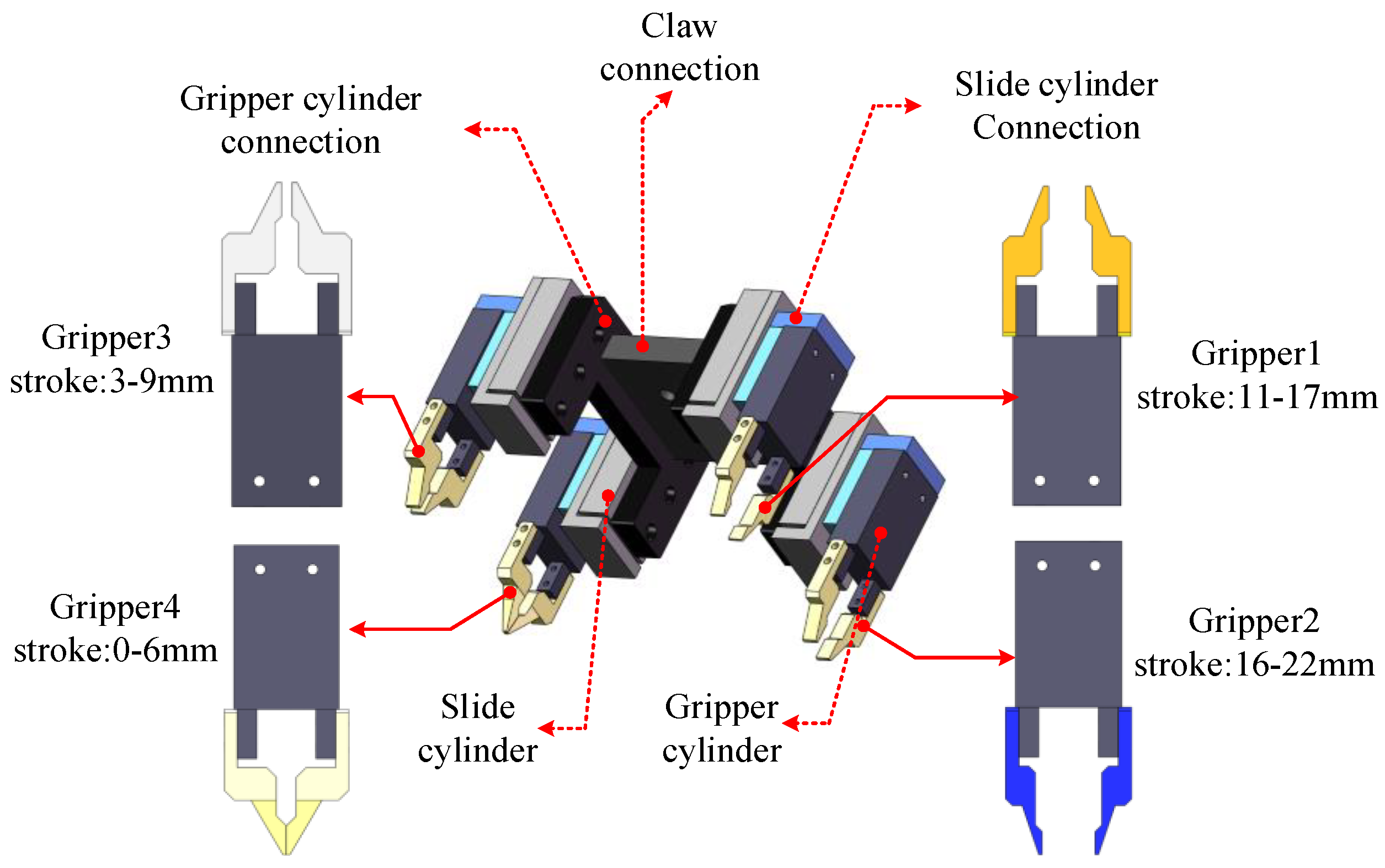
To resolve the high-rigidity problem of existing MCB assembly, this paper proposes a single-robot-based flexible automatic assembly technique that applies a novel multi-gripper claw and a flexible posture adjust scheme to achieve flexible automatic assembly for arc extinguishers, handles, magnetic components and other parts in random varying postures. A time-optimal trajectory optimization method based on improved PSO with a multi-optimization mechanism is proposed. A quintic interpolation polynomial that improves acceleration stability, joint impact and precision is employed. The multi-optimization mechanism based on the fitness switch function is proposed to reduce the computational complexity. Optimization results are judged, compared and optimized according to the fitness switch function to improve efficiency. Meanwhile, an adaptive compression factor is applied to adjust the PSO weights to ensure the global exploration ability of the algorithm in the first stage and the local search ability in the second stage. Finally, the simulation of the PSO algorithm with the time optimality as the objective function is accomplished, and the performances of different algorithms are compared. Experiments are performed on the ROKAE XB4 robot platform, to verify the proposed method.

2. Construction of MCB Flexible Assembly Platform

2.1. Internal Structure of an MCB

The internal structure and the components are shown in Figure 1. In this paper, the handle, the big-U rod, the magnetic yoke, the magnetic system (including a magnetic system rack and a magnetic core), and the arc extinguisher are selected as the objects (as shown in Figure 2) to be assembled by a single robot.

2.2. Process of Robotic Flexible Assembly

A flexible switch control method is proposed. An auxiliary adjustment rack for all parts is designed. The work platform that adjusts random postures of the parts to the specified postures is shown in Figure 3, including a six-axis robot, a flexible multi-gripper claw, an MCB assembly platform, a loading carrier, a positioning carrier, and an auxiliary adjustment rack.

Figure 4 shows the designed flexible multi-gripper claw on the robot. Four grippers with different strokes (11–17 mm, 16–22 mm, 3–9 mm and 0–6 mm, respectively) are designed to match different sizes and assembly requirements of the parts. To effectively hold parts of different sizes and shapes, the ends of the grippers are in specified shapes. The width of the clamping position for the yoke and the magnetic system rack is 1 mm, and that for the big-U rod is 1.2 mm. The connections between the end effector, slider cylinder, and gripper cylinder are also designed. In an adjustment process, the robot automatically chooses a gripper whose stroke range matches the size of the part.

The auxiliary adjustment rack which fixes the parts in specified postures are shown in Figure 5. It is composed of a set of slots as transits to help the part posture adjustment.

Based on the robot assembly platform and the corresponding mechanism shown in Figure 3, Figure 4 and Figure 5, this paper proposes the following flexible assembly method and process of the MCB. Specifically, the arc extinguisher is adjusted by the gripper 1 and 2, the magnetic yoke is adjusted by gripper 3 and 4, the big-U rod is adjusted by gripper 4, and the magnetic system is adjusted by gripper 3 and 4, and the handle is coordinated by gripper 3 and 4. Taking the posture adjustment of the arc extinguisher as an example, the postures are categorized into three situations. The specified process that uses gripper 1 and 2 to adjust the arc extinguisher is shown in Figure 6a. In the case of posture 1, it is rotated around the Z axis by a certain angle by gripper 2, and then placed in the arc extinguisher slot on the positioning carrier. In the case of posture 2, it is clamped by gripper 1 and rotated counterclockwise around the Y-axis and clockwise around Z-axis, and then placed into the auxiliary adjustment rack. Finally, gripper 2 is applied to put it into the arc extinguisher slot. In the case of posture 3, it is clamped by the gripper 1, rotated clockwise around the Y-axis and counterclockwise around the Z-axis, and then placed into the auxiliary adjustment rack. Finally, gripper 2 is applied to put it in the arc extinguisher slot after rotating it around the Z axis.

Figure 6b shows the schematic diagram of posture adjustment of the yoke, big-U rod, magnetic system, and handle. The postures are similarly adjusted as the arc extinguisher in Figure 6a, and finally all the parts are placed in the positioning carrier in specified postures, as shown in Figure 7.

3. Robot Kinematic Modeling

3.1. Robot Kinematic Analysis

This paper employs a ROKAE XB4 six-axis robot whose link structure is shown in Figure 8. The D-H parameters of the robot are shown in

Table 1. D-H parameters.

Joint/i	θi/°	di/m	ai/m	αi/°
1	θ1	0	0	0
2	θ2	0	0.04	−π/2
3	θ3	0	0.275	0
4	θ4	0.28	0.025	−π/2
5	θ5	0	0	π/2
6	θ6	0	0	−π/2

, where θ represents the joint rotation angle, d represents the joint offset, a represents the link length, and α represents the link torsion angle.

In Figure 8, (x_i, y_i, z_i) (I =1,2,3,4,5,6) represent the coordinate system of each joint, while (x₀, y₀, z₀) represents the base coordinate system.

From the four parameters θ_i, a_i, d_i and α_i in Table 1, the homogeneous transformation matrix T_i between adjacent link i and link i−1 is obtained:

$$T_i=\left[\begin{array}{cc}{R}_i& P_i\\ 0& 1\end{array}\right]$$

(1)

where R_i and P_i are the posture matrix and the position matrix between link i and link i−1, respectively:

$$R_i=\left[\begin{array}{ccc}\cos {\theta }_i& -\sin {\theta }_i& 0\\ \sin {\theta }_i\cos {\alpha }_{i-1}& \cos {\theta }_i\cos {\alpha }_{i-1}& -\sin {\alpha }_{i-1}\\ \sin {\theta }_i\sin {\alpha }_{i-1}& \cos {\theta }_i\sin {\alpha }_{i-1}& \cos {\alpha }_{i-1}\end{array}\right]$$

(2)

$$P_i={\left[\begin{array}{ccc}{a}_{i-1}& -\sin {\alpha }_{i-1}{d}_i& \cos {\alpha }_{i-1}{d}_i\end{array}\right]}^T$$

(3)

Substituting Equation (2) and Equation (3) into Equation (1), the homogeneous transformation matrix T₀~T₆ of each joint is obtained. By multiplying the homogeneous transformation matrix T₀~T₆ of each joint, the posture transformation matrix T₀⁶ of the end joint is obtained. Model of the ROKAE XB4 robot created using D-H parameters in Table 1.

3.2. Polynomial Interpolation Function Construction

In the trajectory optimization of the robot, the positions, velocities, accelerations, and jerks of the joints need to be comprehensively considered. This paper employs the quintic (fifth-degree) polynomial which is of a relatively high efficiency for robot trajectory interpolation. The reason for choosing the quintic polynomial is that it balances the performance and the computational complexity. A lower-degree polynomial loses information such as acceleration and jerk, which can cause significant shocks on the joints. A higher-degree polynomial improves the smoothness of the acceleration and jerk, but it is computational expensive and can leads to the Runge phenomenon that distorts the interpolation [16]. The expression is shown in Equation (4).

$$\begin{array}{l}{h}_{j1}(t)=a_{j15}{t}_1^5+a_{j14}{t}_1^4+a_{j13}{t}_1^3+a_{j12}{t}_1^2+a_{j11}{t}_1+a_{j10}\\ h_{j2}(t)=a_{j25}{t}_2^5+a_{j24}{t}_2^4+a_{j23}{t}_2^3+a_{j22}{t}_2^2+a_{j21}{t}_2+a_{j20}\\ h_{j3}(t)=a_{j25}{t}_3^5+a_{j24}{t}_3^4+a_{j23}{t}_3^3+a_{j22}{t}_3^2+a_{j21}{t}_3+a_{j30}\end{array}$$

(4)

where j is the joint number (j = 1,2,3,4,5,6). The unknown coefficients a_j1i, a_j2i, and a_j3i are the i-th coefficients of the first, second, and third segment interpolation functions of the j-th joint trajectory. h_j1(t), h_j2(t), and h_j3(t) respectively represent the quintic polynomial trajectory function of the j-th joint in the third segment, where the variable t_i is the interpolation time, $t_i\in \left\{t_1,t_2,t_3\right\}$.

In the Cartesian system, X_ji is the joint angle calculated by inverse kinematic for the space coordinates of the robotic arm motion. The following conditions of each segment of the j-th joint are given: the starting point X_j0, the intermediate points X_j1 and X_j2, and the ending point X_j3, as well as the acceleration and velocity of the starting and ending points (usually 0); the velocity and acceleration between the path points are continuously equal. According to the known conditions, trajectory coefficient matrix that satisfies the conditions is shown in Equation (5).

$$a=A^{-1}\cdot N$$

(5)

where a is the trajectory curve coefficient solution, A is a polynomial matrix about time t, and N is a matrix of X_ji are shown as follows.

$$A=\left[\begin{array}{ccc}B& C& D\\ E& F& G\\ H& I& J\end{array}\right]$$

(6)

$$\begin{array}{lll}B=\left[\begin{array}{cccccc}1& 0& 0& 0& 0& 0\\ 1& t_1& t_1^2& t_1^3& t_1^4& t_1^5\\ 0& 0& 0& 0& 0& 0\\ 0& 0& 0& 0& 0& 0\\ 0& 0& 0& 0& 0& 0\\ 0& 0& 0& 0& 0& 0\end{array}\right]& C=\left[\begin{array}{cccccc}0& 0& 0& 0& 0& 0\\ 0& 0& 0& 0& 0& 0\\ 1& 0& 0& 0& 0& 0\\ 1& t_2& t_2^2& t_2^3& t_2^4& t_2^5\\ 0& 0& 0& 0& 0& 0\\ 0& 0& 0& 0& 0& 0\end{array}\right]& D=\left[\begin{array}{cccccc}0& 0& 0& 0& 0& 0\\ 0& 0& 0& 0& 0& 0\\ 0& 0& 0& 0& 0& 0\\ 0& 0& 0& 0& 0& 0\\ 1& 0& 0& 0& 0& 0\\ 1& t_3& t_3^2& t_3^3& t_3^4& t_3^5\end{array}\right]\\ E=\left[\begin{array}{cccccc}0& 1& 0& 0& 0& 0\\ 0& 1& 2t_1& 3t_1^2& 4t_1^3& 5t_1^4\\ 0& 0& 0& 0& 0& 0\\ 0& 0& 0& 0& 0& 0\\ 0& 0& 1& 0& 0& 0\\ 0& 0& 1& 3t_1& 6t_1^2& 10t_1^3\end{array}\right]& F=\left[\begin{array}{cccccc}0& -1& 0& 0& 0& 0\\ 0& 1& 2t_2& 3t_2^2& 4t_2^3& 5t_2^4\\ 0& 0& 0& 0& 0& 0\\ 0& 0& 0& 0& 0& 0\\ 0& 0& 0& 0& 0& 0\\ 0& 0& -1& 0& 0& 0\end{array}\right]& G=\left[\begin{array}{cccccc}0& 0& 0& 0& 0& 0\\ 0& 0& 0& 0& 0& 0\\ 0& -1& 0& 0& 0& 0\\ 0& 1& 2t^3& 3t_2^3& 4t_2^3& 5t_2^4\\ 0& 0& 0& 0& 0& 0\\ 0& 0& 0& 0& 0& 0\end{array}\right]\\ H=\left[\begin{array}{cccccc}0& 0& 0& 0& 0& 0\\ 0& 0& 0& 0& 0& 0\\ 0& 0& 0& 1& 0& 0\\ 0& 0& 0& 1& 4t_1& 10t_1^2\\ 0& 0& 0& 0& 0& 0\\ 0& 0& 0& 0& 0& 0\end{array}\right]& I=\left[\begin{array}{cccccc}0& 0& 1& 3t_2& 6t_2^2& 10t_2^3\\ 0& 0& 0& 0& 0& 0\\ 0& 0& 0& 0& 0& 0\\ 0& 0& 0& -1& 0& 0\\ 0& 0& 0& 1& 4t_2& 10t_2^2\\ 0& 0& 0& 0& 0& 0\end{array}\right]& J=\left[\begin{array}{cccccc}0& 0& -1& 0& 0& 0\\ 0& 0& 1& 3t_3& 6t_3^2& 10t_3^3\\ 0& 0& 0& 0& 0& 0\\ 0& 0& 0& 0& 0& 0\\ 0& 0& 0& -1& 0& 0\\ 0& 0& 0& 1& 4t_3& 10t_3^2\end{array}\right]\end{array}$$

(7)

$$N={\left[\begin{array}{ccccccccc}{X}_{j1}& X_{j2}& X_{j2}& X_{j3}& X_{j3}& X_{j4}& 0& \cdots & 0\end{array}\right]}_{1\times 18}^T$$

(8)

4. Particle Swarm Time Optimal Trajectory Planning

4.1. Time-Optimal Trajectory Planning

Trajectory planning is to design the joint motion curve of the robot according to the robot’s operating requirements. In the planning process, it is required to satisfy the constraints of robot kinematic, dynamics, and the surrounding environment of the robot, and comprehensively consider the smoothness of joint motion, running time and energy consumption. The trajectory planning space of industrial robots can be divided into two types, the joint space and the Cartesian space. Since trajectory planning in the joint space can ensure the smoothness of joint motions by reducing the positioning accuracy of the robot arm Cartesian space, and the robot arm motion trajectory in the Cartesian space have problems such as singular points and joint redundancy, this paper chooses the joint space trajectory planning method. The process of joint space trajectory planning is based on two groups of six joint angles obtained by inverse kinematics, inserting multiple points between the starting and ending points within the interpolation curve, to fit the function curve of the joint angle with a time optimal strategy. Hence, each joint of the robot operates through the joint angle function. The first, second, and third derivatives of the joint angle function are the velocity, acceleration, and jerk, respectively. The maximum speed, acceleration and jerk of the robot joints are adjusted and optimized by the joint motion constraint conditions, so that the time optimal motion control can be achieved.

The goal of trajectory planning in this paper is to find the time-optimal trajectory in the joint space with multiple constraints. By analyzing the assembly path of the robot, the starting and ending points of the path are selected. Based on the actual motion constraint conditions (speed, acceleration, jerk), the joint angle function curve is optimized by ensuring the motion smoothness.

4.2. Improved PSO Algorithm

This paper seeks the optimal trajectory by an improved particle swarm optimization (PSO) algorithm with the objective function of time. Suppose that in a D-dimensional search space, a population $X=(X_1,X_2,\cdots ,X_n)$ composed of n particles, where the i-th particle is represented as a D-dimensional vector $X_i={(x_{i1},x_{i2},\cdots ,x_{in})}^T$, which represents the position of the i-th particle, i.e., a potential solution. The fitness corresponding to each particle position X_i can be calculated by the objective function. The velocity of the i-th particle is $V_i={(V_{i1},V_{i2},\cdots ,V_{iD})}^T$, the individual extreme value is $P_i={(P_{i1},P_{i2},\cdots ,P_{iD})}^T$, and the population extreme value of the population is $P_g={(P_{g1},P_{g2},\cdots ,P_{gD})}^T$. In each iteration, the particle updates its speed and position by extreme values of the individual and the group, as shown below:

$$V_{{}_{id}}^{{}^{k+1}}=\omega V_{{}_{id}}^k+c_1{r}_1(P_{id}^k-X_{id}^k)+c_2{r}_2(P_{gd}^k-X_{id}^k)$$

(9)

$$X_{{}_{id}}^{{}^{k+1}}=X_{id}^k+V_{id}^{k+1}$$

(10)

where ω is the inertia weight, $d=1,2,\cdots ,D$, $i=1,2,\cdots ,n$, and k are the current iteration times; V_id is the particle velocity; c₁ and c₂ are acceleration factors (non-negative constants); r₁ and r₂ are random numbers (distributed within [0, 1]). To prevent the blind search of particles, the position $X_{id}^k$ is within [−X_max, X_max], and the speed $V_{id}^k$ is within [−0.1·X_max, 0.1·X_max].

The key of PSO with the quintic polynomial interpolation is to obtain the optimal time $x_{id}^k$ by selecting the independent variables for particle optimization. This paper performs optimization in the search space of time t₁, t₂, and t₃ by reducing the number of search dimensions of the particle swarm to three to avoid complex mapping relations in the derivation. Meanwhile, multi-optimization is with the fitness switch function are applied to improve the converge speed. Time-optimal optimization iteration is performed after the kinematic constraints are met. The fitness function is described as follows:

$$f\left(t\right)=min\left(t_1+t_2+t_3\right)$$

(11)

$$\begin{array}{l}s.t.\max \left\{\right|V_{j1}\left|\right\}\le V_{\max }\\ \max \left\{\right|V_{j2}\left|\right\}\le V_{\max }\\ \max \left\{\right|V_{j3}\left|\right\}\le V_{\max }\end{array}$$

(12)

where V_j1, V_j2, V_j3, and V_max are the real-time speed and maximum speed limits of the i-th joint, respectively.

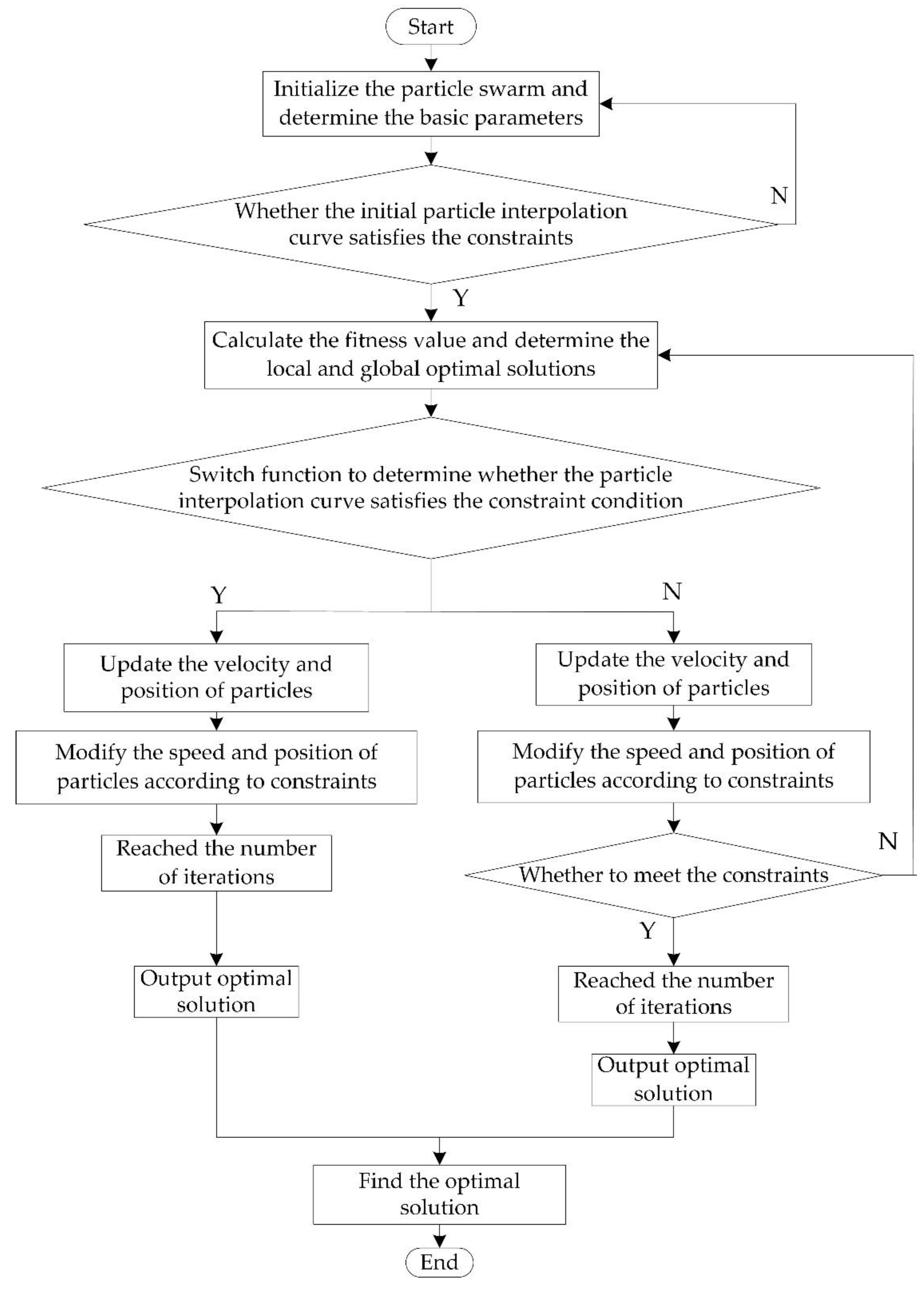
This paper introduces multi-optimization mechanisms into the PSO algorithm. In the multi-optimization process, a conditional judgment optimization mechanism based on the fitness switch function is proposed, and the corresponding fitness switch function is established according to the result of the particle fitness. Therefore, the result is judged, compared and optimized according to the fitness switch function. The improved PSO process in this article is shown in Figure 9.

Compared with the standard particle swarm optimization process, this paper introduces two optimization processes in the standard PSO algorithm to form a multi-optimization mechanism. A conditional decision mechanism based on a fitness switch function in the multi-optimization process, As shown in Figure 9. On one hand, after initializing the particle swarm and determining the basic parameters, the interpolation period of the initialized particles is selected according to the constraints to prevent the initial randomness which reduce the optimization efficiency. Therefore, the rationality of each initial particle can be guaranteed; on the other hand, after the particle fitness, the current individual extreme value and the group extreme value are determined, a fitness switch function that quickly finds the optimal is used to select the particles. The function is defined as follows:

$$f_{fitness}\left(t\right)=\{\begin{array}{c}{f}_1\left(t\right),(\forall V_{j1}(t),\forall V_{j2}(t),\forall V_{j3}(t)\le V_{\max })\\ f_2\left(t\right),(\exists V_{j1}(t),\exists V_{j2}(t),\exists V_{j3}(t)>V_{\max })\end{array}$$

(13)

$$f_1\left(t\right)=min\left(t_1+t_2+t_3\right)$$

(14)

$$f_2(t)=\min \{\begin{array}{c}{e}_1+t_2+t_3(\exists V_{j1}(t)>V_{\max })\\ t_1+e_2+t_3(\exists V_{j2}(t)>V_{\max })\\ t_1+t_2+e_3(\exists V_{j3}(t)>V_{\max })\\ t_1+e_2+e_3(\exists V_{j2}(t),\exists V_{j3}(t)>V_{\max })\\ e_1+t_2+e_3(\exists V_{j1}(t),\exists V_{j3}(t)>V_{\max })\\ e_1+e_2+t_3(\exists V_{j1}(t),\exists V_{j2}(t)>V_{\max })\\ e_1+e_2+e_3(\exists V_{j1}(t),\exists V_{j2}(t),\exists V_{j3}(t)>V_{\max })\end{array}$$

(15)

where t₁, t₂, and t₃ are the interpolation times of the robot; e₁, e₂, and e₃ are the interpolation times when the constraints are not met during the iteration process; V_j1, V_j2, and V_j3 are the velocities of the j-th joint, respectively.

As shown in Equation (13), the fitness switch function conditionally selects the particle fitness in segments. If the velocities of the three segments meet the constraints of Equation (12), the fitness calculation of f₁(t) in Equation (13) will be performed and followed by iterations; otherwise, the particles will be re-constrained and optimized based on the constraint conditions of equation. To guarantee the stability of the interpolated curve, the velocities are reduced until the requirements of f₂(t) in Equation (15). Equation (15) represents the seven calculation situations of f₂(t). Aiming at the above-mentioned seven conditions of inconformity, the time variables e₁, e₂, and e₃ are employed. The fitness switch function sifts and categorizes the particles into two types: superior particles which meet all constraints and can be directly optimized for iterations (the “Y” branch); inferior particles which cannot fully meet the constraints and need to be modified before the iterations (the “N” branch).

The optimization parameters are as follows: the particle swarm number m = 50; the initial particle position is a random number within [0, 5]; the maximum flying speed of the particle is within [−0.5, 0.5]. An adaptive compression factor is added to PSO, to adjust the weight of the PSO algorithm to guarantee the initial global search capability and the later local search capability, The particle swarm velocity update equation is shown in Equation (16):

$$V=\phi (\omega V_{{}_{id}}^k+c_1{r}_1(P_{id}^k-X_{id}^k)+c_2{r}_2(P_{gd}^k-X_{id}^k))$$

(16)

$$\phi ={\mu }^{e^{\frac{1-iterofcur}{NGer+1-iterofcur}}-1}$$

(17)

$\phi$ is the adaptive compression factor, iterofcur is the current number of iterations, NGer is the total number of iterations (set to 100), $\mu$ is a positive integer (set to 8), e is a positive integer of (set to 10), the weight $\omega$ is 0.5, and the weight factor c₁ = 2, c₂ = 2, r₁ and r₂ are random numbers within [0, 1].

5. Algorithm Simulation

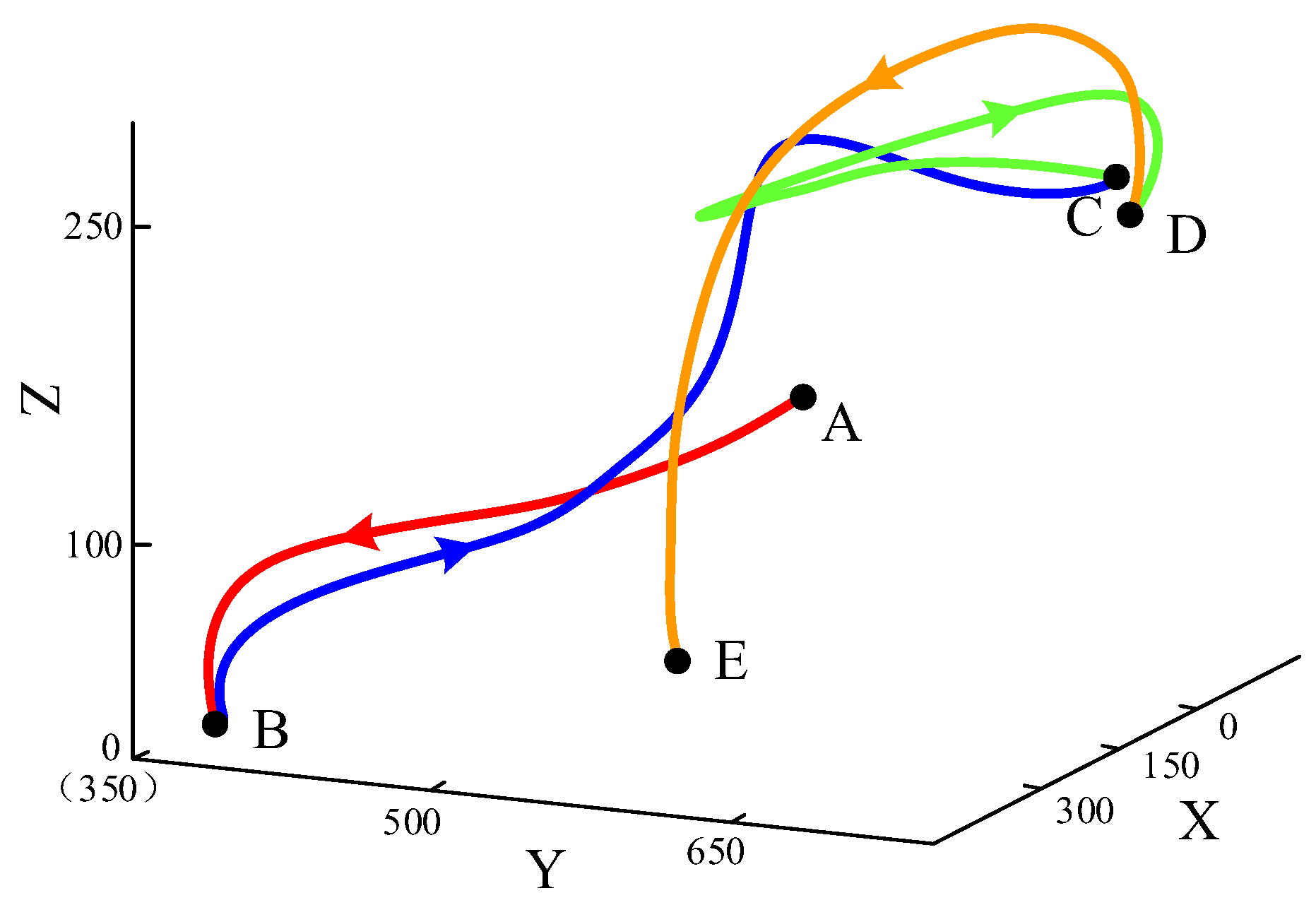
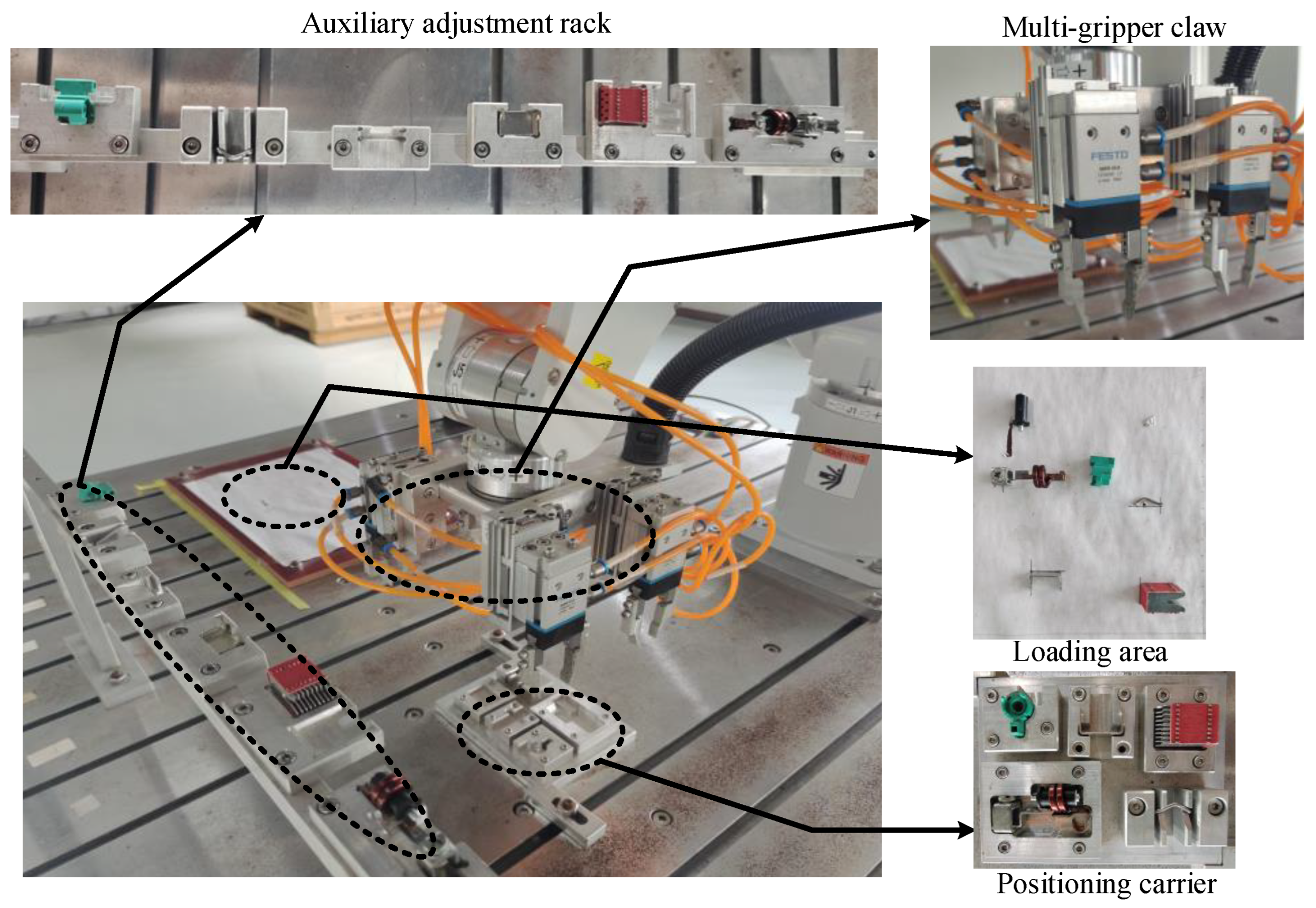
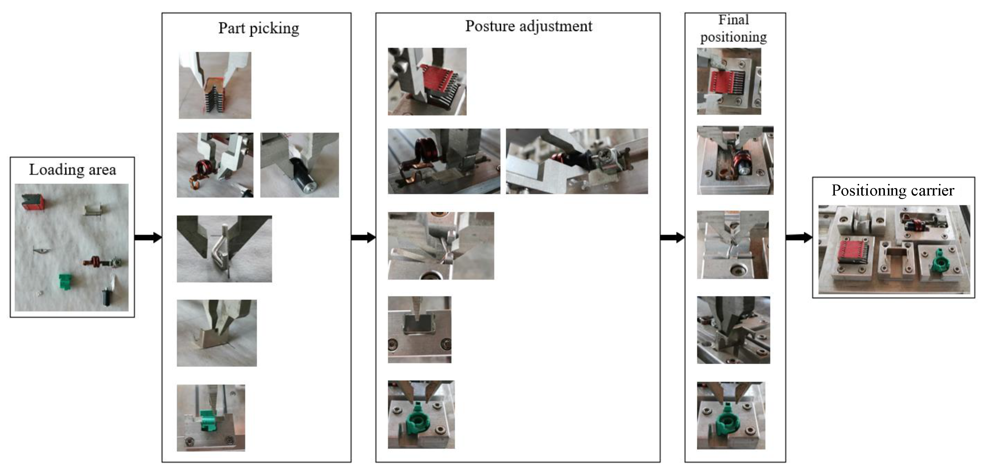
As shown in Figure 10, the flexible assembly performed of MCB parts can be divided into four operating sections: section AB represents the robot moving from the initial position to the loading area; section BC represents the robot gripping a part and placing it on the adjustment rack; section CD indicates the robot adjusting the part to a fixed posture for assembly on the adjustment rack; section DE indicates the robot arm placing the adjusted part on the positioning carrier.

This paper takes section AB as an example for optimization verification. The interpolation points and interpolation times of the six joints are shown in

Table 2. Interpolation points of the joints.

Point/Xi	Joint 1	Joint 2	Joint 3	Joint 4	Joint 5	Joint 6
X1/(°)	0	−35.1	−29.8	0	−25.1	0
X2/(°)	−24	−37.7	−30.6	0	−21.7	23.96
X3/(°)	−43.7	−52.2	−4.14	0	−33.6	135.3
X4/(°)	−30	−58.3	−2.11	0	−29.6	125

and

Table 3. Interpolation times of the joints.

ti/(s)	t1	t2	t3
Interpolation time	3.0	6.0	3.0

, and the joint kinematic constraints are shown in

Table 4. Joint kinematic constraints.

Joint/i	Joint 1	Joint 2	Joint 3	Joint 4	Joint 5	Joint 6
p/(o)	−43.7	−58.3	−30.6	0.00	−33.6	135.3
v/(rad/s)	0.90	0.90	0.90	0.90	0.95	1.00
a/(rad/s2)	0.90	0.90	0.90	0.90	0.90	1.00
a’/(rad/s3)	2.00	2.00	2.00	2.00	2.00	2.00

. During the process of section AB, joint 4 has no angular deflection, so the angle difference is 0 degrees.

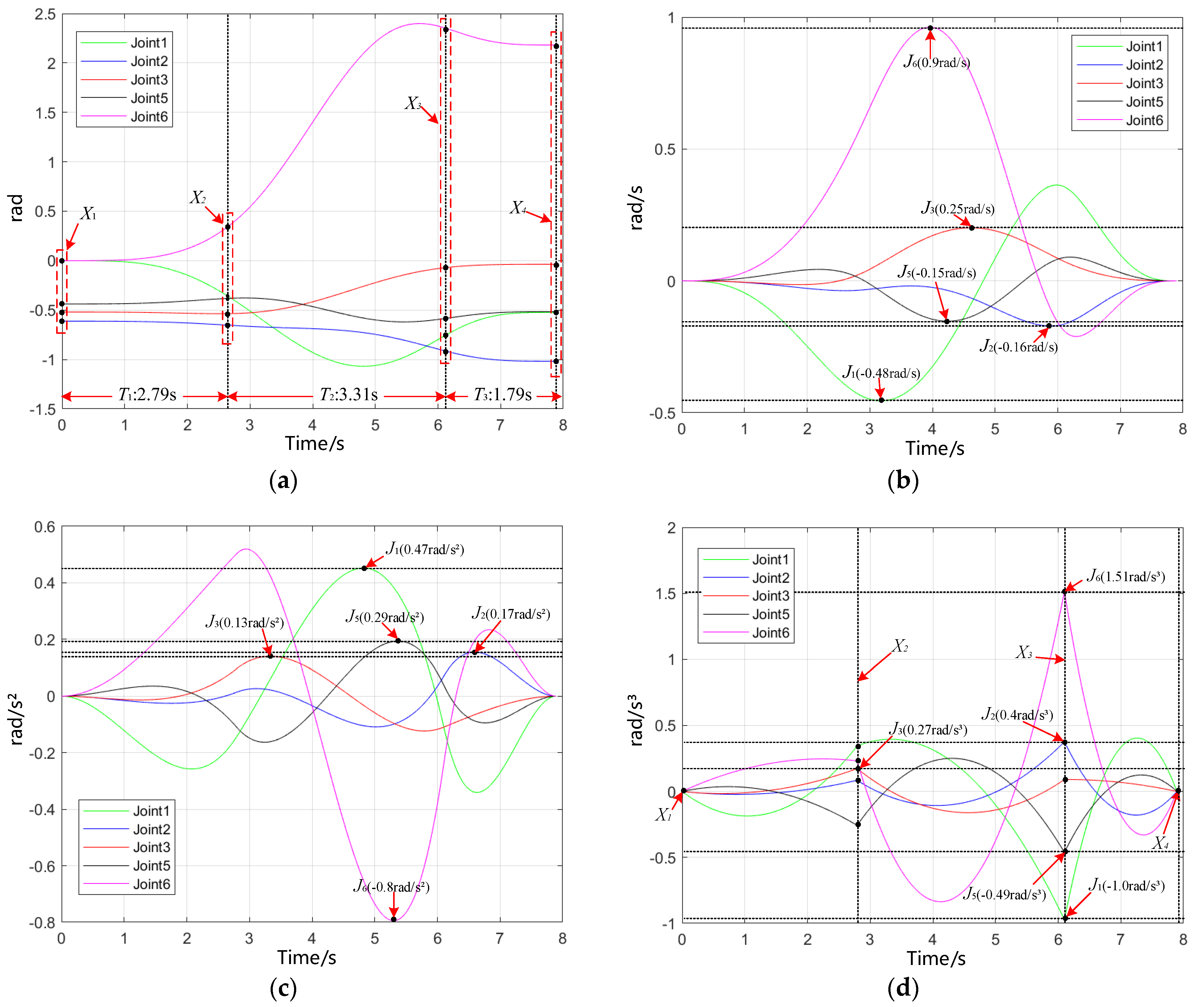
The position, velocity, acceleration, and jerk interpolation curves of the six joints calculated by the first quintic polynomial interpolation are shown in Figure 11. In Figure 11, The oscillations of the position, speed, and acceleration curves are expected to be continuous and smooth. Meanwhile, the maximum values of the speed, acceleration, and jerk oscillations are expected to be as close to the constraint values as possible, to achieve a higher performance. Figure 11a shows that the quintic polynomial interpolation curve passes the given interpolation points X₁, X₂, X₃, X₄ and is continuously smooth during t₁, t₂, and t₃, which proves the effectivity of the fifth-degree polynomial interpolation. Figure 11b–d show that the unoptimized speed, acceleration, and jerk curves are continuous, and the peaks meet the constraints Table 4, but the maximum values of the oscillations are much smaller than the constraint values.

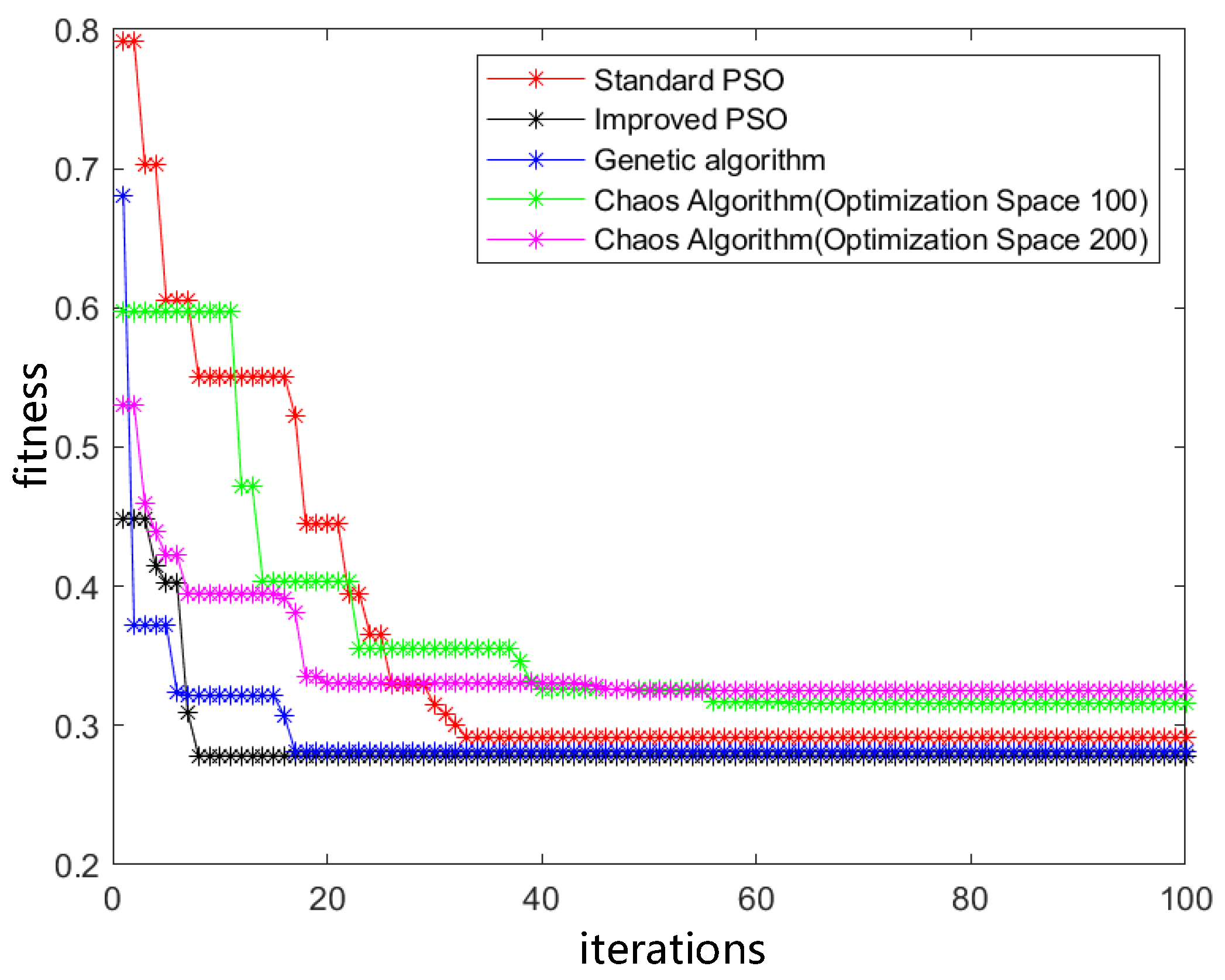
To compare and verify the optimization results, the proposed optimization algorithm is compared with the standard PSO, genetic algorithm (GA), and chaotic optimization algorithm (COA). The chaotic optimization algorithm designed two different optimization spaces, and the comparison results are shown in Figure 12, which shows that the improved PSO converges to the optimal at the 8th iteration, the standard PSO converges to the optimal value at the 33rd iteration, the genetic algorithm converges to the optimal at the 17th iteration, and the COA with optimization space sizes of 100 and 200 converges to the optimal value at the 20th and 56th iteration, respectively. Hence, the improved PSO is about 76% faster than the standard PSO, 53% faster than the genetic algorithm, and 60% and 85.7% faster than the chaos algorithm. According to the fitness, the improved PSO raises the optimization accuracy by 1.1%, 4.4%, 15.7%, and 12.2%, respectively, compared with other algorithms. Since the chaos optimization algorithm decreases significantly as the optimization space increases, the improved PSO has significantly improved convergence speed and convergence accuracy when the optimization space increases compared to the chaotic algorithm.

The running time of each joint in section AB optimized by the improved PSO algorithm is shown in

Table 5. Time before and after the optimization of section AB.

Joint/i	ti1/s		ti2/s		ti3/s
	Standard	Improved	Standard	Improved	Standard	Improved
Joint1	3.00	2.79	1.43	1.29	1.90	1.68
Joint2	0.38	0.30	0.68	0.54	0.70	0.56
Joint3	0.63	0.46	1.98	1.67	0.58	0.45
Joint4	0.00	0.00	0.00	0.00	0.00	0.00
Joint5	0.81	0.67	1.15	0.88	0.85	0.71
Joint6	1.95	1.88	3.34	3.31	1.85	1.79
Optimal	3.00	2.79	3.34	3.31	1.90	1.79

.

Since the joints move simultaneously during the operation of the robot, the interpolation time of each section in Table 4 is the maximum value of the joints. Therefore, t₁ = 2.79 s, t₂ = 3.31 s, t₃ = 1.79 s. Comparing the running time before optimization in Table 3, the overall time of section AB is decreased from 12 s to 7.89 s, i.e., decreased by 34.25%.

The optimized position, velocity, acceleration, and jerk curves of the six joints are shown in Figure 13. The optimized joint curve also passes through the interpolation points X₁, X₂, X₃, and X₄, and meets the kinematic constraints in Table 4. The extreme values of the curves become closer to the constraints, and the acceleration curve is continuous and stable. Figure 13c shows that the maximum acceleration of the joints is 0.8 rad/s² which is within the acceleration constraint range of Table 3. Figure 13d shows that the maximum jerk of the joints is 1.51 rad/s³ which is within the jerk constraint range in Table 3. Hence, it can be concluded that the improved PSO decreases the assembly time and raises the operation efficiency.

After the optimization, the time comparison of the four paths is shown in

Table 6. Times of the four sections before and after the algorithm is improved (unit: s).

Section	No Optimization			Standard PSO			Standard GA			Standard COA			Improved PSO
	t1	t2	t3	t1	t2	t3	t1	t2	t3	t1	t2	t3	t1	t2	t3
AB	3	6	3	3.00	2.79	3.34	3.04	2.53	3.77	3.43	3.01	2.88	3.31	1.90	1.79
BC	8	5	8	4.03	1.80	7.31	5.13	3.22	6.97	4.75	2.06	5.83	4.10	1.63	5.80
CD	3	6	8	3.00	5.49	4.11	2.89	4.51	4.34	2.51	5.17	4.40	2.46	4.89	3.30
DE	7	3	3	3.54	1.55	1.27	4.01	1.70	1.62	3.87	1.50	1.11	2.82	1.28	1.05

.

It can be seen from Table 6 that after the improved PSO algorithm is applied, the times of the four sections are decreased by 2.13 s, 1.61 s, 1.95 s, and 1.21 s, respectively, and the overall time is decreased by 6.90 s, compared with those before PSO improvement, i.e., the overall efficiency is increased by 16.7%. In addition, we also implement the standard generic algorithm (GA) and chaotic optimization algorithm (COA) whose parameters are tuned to the optimal for comparison, and obviously our method is superior to the standard GA and COA.

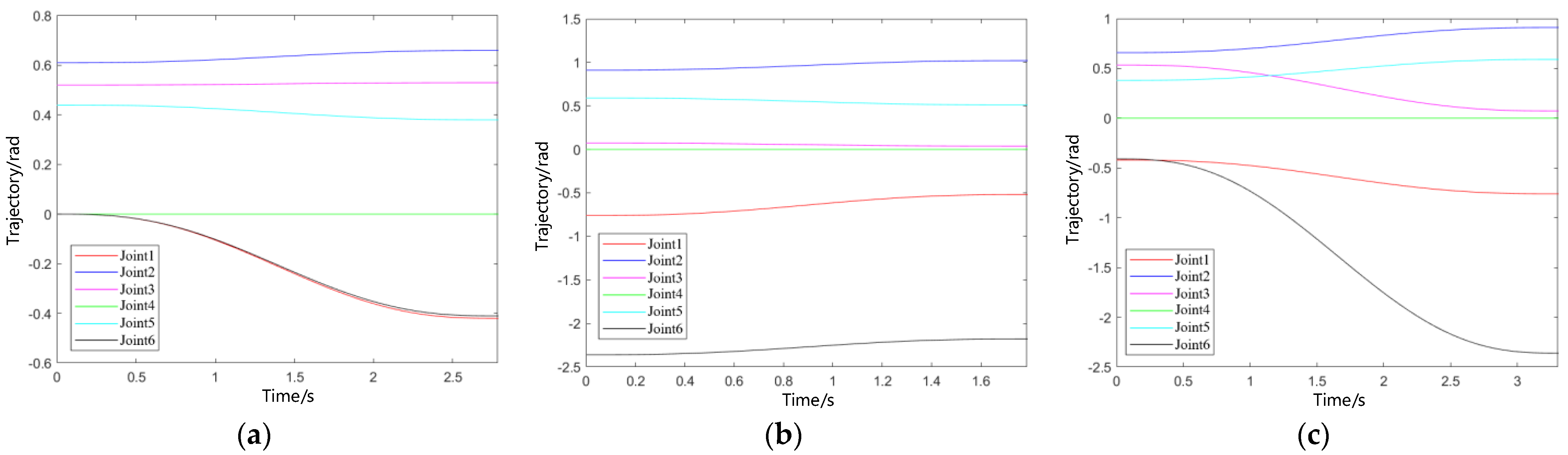
Figure 14 shows the simulation curves of the robot joint trajectory planning, illustrating the interpolation curves of the three-segment times t₁, t₂, and t₃ after the optimization. It can be observed that the interpolation trajectory as well as the operating curves are continuous, smooth, and stable. Meanwhile, the operating time completely corresponds to the final optimized times t₁, t₂, and t₃. Experiments prove the effectiveness of the improved PSO for time-optimal trajectory planning.

6. Experiment on the Assembly Platform

Figure 15 shows the experimental posture adjustment platform for flexible assembly, including a six-axis robot with a flexible multi-gripper claw, a positioning carrier, a loading area, an auxiliary adjustment rack, etc. Based on the flexible assembly process designed in Chapter 1, in the flexible assembly experiment verification, the mechanical arm clamps the MCB parts in random postures from the loading area. After the posture adjustment of the auxiliary adjustment rack, the part is placed in the positioning carrier in the final posture. The complete assembly process is illustrated in Figure 16, which illustrates the processes that the robot picks randomly postured parts from the loading area, places them in the corresponding adjustment slots on the auxiliary adjustment rack, re-picks them from the slots and lays them on the positioning carrier. Because of the different shapes of the parts, the trajectories for each part are different.

Table 7. Comparison of operating times of different parts on the experimental platform (unit: s).

Part	Section	No Optimization	Standard PSO	Improved PSO
Arc extinguisher	AB	9.34	16.43	9.08
	BC	15.36	14.54	12.85
	CD	11.06	4.64	5.85
	DE	12.52	8.03	12.75
	Total	48.28	43.63	40.53
Big-U rod	AB	12.76	13.88	12.68
	BC	11.84	9.00	9.05
	CD	15.04	14.63	11.23
	DE	11.06	11.39	14.45
	Total	50.70	48.89	47.40
Yoke	AB	10.22	13.50	7.43
	BC	14.64	11.90	15.33
	CD	12.18	12.62	10.30
	DE	12.10	9.65	8.33
	Total	49.14	47.68	41.38
Handle	AB	12.48	12.65	9.90
	BC	13.90	9.29	10.45
	CD	12.86	9.36	9.75
	DE	8.34	11.68	9.68
	Total	47.58	42.98	39.78

shows the robot’s operating times for picking, adjusting and poisoning different parts on the experimental platform. The parts are randomly placed in the loading area and the postures are given by a machine vision system. We compared the results around no optimization, the standard PSO and the improved PSO, and it is proven that the proposed method achieves the smallest operating time.

7. Conclusions

This paper proposes a flexible automatic assembly technique to solve the high rigidity issue in current MCB manufacturing, and realizes the flexible automatic assembly of multiple MCB parts with a single robot. A time-optimal trajectory PSO method with a multi-optimization mechanism is proposed. A fitness switch function that judges, compares, and optimizes the results is employed to improve the calculation efficiency. Simulation and experimental results show that compared with other methods, the proposed improved PSO significantly raise the accuracy and efficiency of the robot trajectory planning.

However, the proposed trajectory planning method is developed for the purpose of MCB assembly and is proven on our specifically designed experimental platform. The practicability cannot be fully proven by the experimental results since the conditions of manufacturing are more severe and complicated. Therefore, there are several issues to be improved in the future work: Firstly, the proposed method is expected to be applied to other robotic applications, as well as to different types of industrial robots, e.g., parallel robots, SCARA robots, for a validation of generality; Secondly, it is expected that the proposed method works under the condition that the robot operating with its maximum power, i.e., the fastest motion, and so that to inspect the performance of the proposed method; Thirdly, the cooperating system of the robot and a machine vison device is expected to be established in the next step, to automatically identify and adjust randomly postured parts.

References

1. Rudsari, F.N.; Razi-Kazemi, A.A.; Shoorehdeli, M.A. Fault Analysis of High-Voltage Circuit Breakers Based on Coil Current and Contact Travel Waveforms Through Modified SVM Classifier. IEEE Trans. Power Deliv. 2019, 34, 1608–1618. [Google Scholar] [CrossRef]
2. Sun, S.; Wen, Z.; Du, T.; Wang, J.; Tang, Y.; Gao, H. Remaining Life Prediction of Conventional Low-Voltage Circuit Breaker Contact System Based on Effective Vibration Signal Segment Detection and MCCAE-LSTM. IEEE Sens. J. 2021, 21, 21862–21871. [Google Scholar] [CrossRef]
3. Shi, X.; Zhang, F.; Qu, X.; Liu, B. An Online Real-Time Path Compensation System for Industrial Robots Based on Laser Tracker. Int. J. Adv. Robot. Syst. 2016, 13, 1729881416663366. [Google Scholar] [CrossRef]
4. He, M.; Wu, X.; Shao, G.; Wen, Y.; Liu, T. A Semiparametric Model-Based Friction Compensation Method for Multi-Joint Industrial Robot. J. Dyn. Syst. Meas. Control 2022, 144, 034501. [Google Scholar] [CrossRef]
5. Hu, J.; Zhu, Q. Multi-Objective Mobile Robot Path Planning Based on Improved Genetic Algorithm. In Proceedings of the 2010 International Conference on Intelligent Computation Technology and Automation, Changsha, China, 11–12 May 2010. [Google Scholar]
6. Jun, H.; Li, H. Trajectory Planning and Simulation of Robot in Joint Coordinate System. J. Nanjing Univ. Sci. Technol. 2000, 24, 540–543. [Google Scholar]
7. Fu, X.G.; Yan, G.Z. Trajectory Planning and Simulating on 7-DOF Robot Applied to Nuclear Industry. Acta Simulata Syst. Sin. 2005, 17, 1948–1950. [Google Scholar]
8. Abu-Dakka, F.J.; Valero, F.J.; SuñEr, J.L.; Mata, V. A Direct Approach to Solving Trajectory Planning Problems Using Genetic Algorithms with Dynamics Considerations in Complex Environments. Robotica 2015, 33, 669–683. [Google Scholar] [CrossRef]
9. Choi, Y.K.; Park, J.H.; Kim, H.S. Optimal Trajectory Planning and Sliding Mode Control for Robots Using Evolution Strategy. Robotica 2000, 18, 423–428. [Google Scholar] [CrossRef]
10. Zhu, S. Time-Optimal and Jerk-Continuous Trajectory Planning Algorithm for Manipulators. J. Mech. Eng. 2010, 46, 456–462. [Google Scholar] [CrossRef]
11. Bukata, L.; Šůcha, P.; Hanzálek, Z. Optimizing Energy Consumption of Robotic Cells by a Branch & Bound Algorithm. Comput. Oper. Res. 2019, 102, 52–66. [Google Scholar] [CrossRef]
12. Rubio, F.; Llopis-Albert, C.; Valero, F.; Suñer, J.L. Industrial Robot Efficient Trajectory Generation without Collision through the Evolution of the Optimal Trajectory. Robot. Auton. Syst. 2016, 86, 106–112. [Google Scholar] [CrossRef]
13. Huang, T.; Zhao, D.; Cao, Z.-C. Trajectory Planning of Optical Polishing Based on Optimized Implementation of Dwell Time. Precis. Eng. 2020, 62, 223–231. [Google Scholar] [CrossRef]
14. Kim, K.W.; Kim, H.S.; Choi, Y.K.; Park, J.H. Optimization of Cubic Polynomial Joint Trajectories and Sliding Mode Controllers for Robots Using Evolution Strategy. In Proceedings of the IECON’97 23rd International Conference on Industrial Electronics, Control, and Instrumentation (Cat. No. 97CH36066), New Orleans, LA, USA, 14 November 1997. [Google Scholar]
15. Ma, Y.; Liang, Y. An Obstacle Avoidance Algorithm for Manipulators Based on Six-Order Polynomial Trajectory Planning. Xibei Gongye Daxue Xuebao/J. Northwest. Polytech. Univ. 2020, 38, 392–400. [Google Scholar] [CrossRef]
16. Trefethen, L.N. Approximation Theory and Approximation Practice, Extended Edition; Other Titles in Applied Mathematics; Society for Industrial and Applied Mathematics: Philadelphia, PA, USA, 2019; ISBN 978-1-61197-593-2. [Google Scholar]
17. Guan, C.; Wang, F.; Zhang, D.Y. NURBS-Based Time-Optimal Trajectory Planning on Robotic Excavators. J. Jilin Univ. Technol. Ed. 2015, 45, 540–546. [Google Scholar]
18. Liang, H.B.; Wang, Y.Z.; Li, X. Research and Implementation of NURBS Interpolation Algorithm for Adaptive Feed Speed. Comput. Integr. Manuf. Syst. 2006, 12, 428. [Google Scholar]
19. Huang, J.; Hu, P.; Wu, K.; Zeng, M. Optimal Time-Jerk Trajectory Planning for Industrial Robots. Mech. Mach. Theory 2018, 121, 530–544. [Google Scholar] [CrossRef]
20. Ajayi, E.; Obe, O. Genetic Algorithm Based Optimal Trajectories Planning for Robot Manipulators on Assigned Paths. Int. J. Emerg. Trends Technol. Comput. Sci. 2020, 8, 4888–4892. [Google Scholar] [CrossRef]
21. Yan, C.; Song, L.I.; Liu, Y. Tool Axis Trajectory Planning for Flank Milling with Conical Tools Based on Particle Swarm Optimization. Comput. Integr. Manuf. Syst. 2016. [Google Scholar] [CrossRef]
22. Yang, H.; Yang, Z.; Yang, Y.; Zhang, L. An Improved Particle Swarm Optimization Algorithm Based on Simulated Annealing. In Proceedings of the 2014 10th International Conference on Natural Computation (ICNC), Xiamen, China, 19–21 August 2014. [Google Scholar]
23. Shen, L.; Wang, Y.; Liu, K.; Yang, Z.; Shi, X.; Yang, X.; Jing, K.; Talley, W. Synergistic Path Planning of Multi-UAVs for Air Pollution Detection of Ships in Ports. Transp. Res. Part E Logist. Transp. Rev. 2020, 144, 102128. [Google Scholar] [CrossRef]
24. Shi, B.; Xu, J. Time-Optimal Trajectory Planning of Industrial Robot Based on Improved Particle Swarm Optimization Algorithm. In Proceedings of the 2020 39th Chinese Control Conference (CCC), Shenyang, China, 27–30 July 2020; pp. 3683–3688. [Google Scholar]
Figure 1. Internal structure of an MCB.
Algorithms 15 00269 g001
Figure 2. Models of the parts to be assembled.
Algorithms 15 00269 g002
Figure 3. Posture adjustment platform.
Algorithms 15 00269 g003
Figure 4. Robot flexible multi-gripper claw.
Algorithms 15 00269 g004
Figure 5. Auxiliary adjustment rack for the parts.
Algorithms 15 00269 g005
Figure 6. Flexible assembly processes for the parts: (a) arc extinguishing cover posture adjustment; (b) position adjustment of other parts.
Algorithms 15 00269 g006
Figure 7. Positioning carrier with adjusted parts.
Algorithms 15 00269 g007
Figure 8. Schematic diagram of the robot connecting rod structure.
Algorithms 15 00269 g008
Figure 9. Improve PSO process.
Algorithms 15 00269 g009
Figure 10. Schematic diagram of robot segmentation.
Algorithms 15 00269 g010
Figure 11. Joint motions before optimization: (a) Position curve; (b) Velocity curve; (c) Acceleration curve; (d) Jerk curve.
Algorithms 15 00269 g011
Figure 12. Comparison of iterative process before and after PSO algorithm improvement.
Algorithms 15 00269 g012
Figure 13. Joint motions after optimization: (a) Position curve; (b) Velocity curve; (c) Acceleration curve; (d) Jerk curve.
Algorithms 15 00269 g013
Figure 14. Time-optimal trajectory planning by the improved PSO: (a) section AB t1 trajectory; (b) section AB t2 trajectory; (c) section AB t3 trajectory.
Algorithms 15 00269 g014
Figure 15. Experimental platform of posture adjustment.
Algorithms 15 00269 g015
Figure 16. Flexible assembly experiment.
Algorithms 15 00269 g016