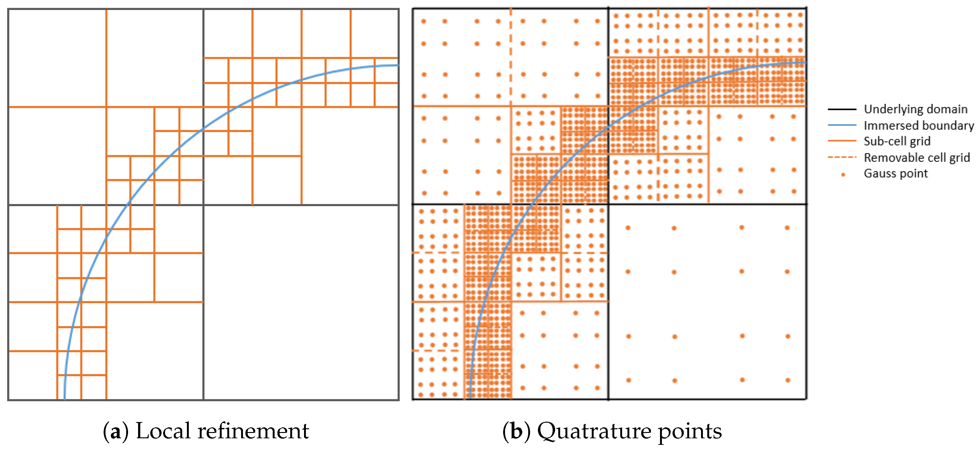
Figure 1.
Illustration of (a) refinement of fields and (b) their associated quadrature points near immersed boundaries.
Figure 1.
Illustration of (a) refinement of fields and (b) their associated quadrature points near immersed boundaries.
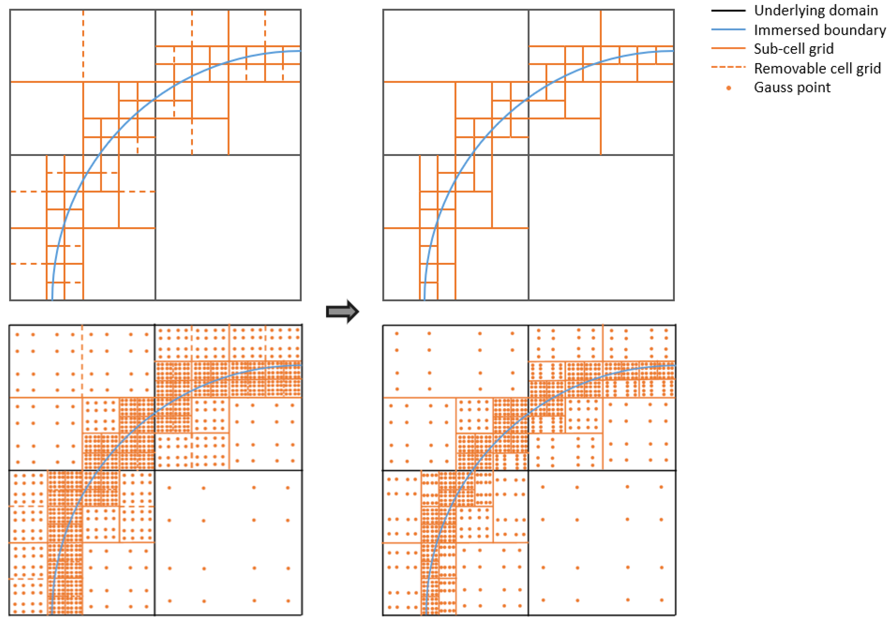
Figure 2.
Illustration of sub-cell coalescence when removing non-intersected cell grids.
Figure 2.
Illustration of sub-cell coalescence when removing non-intersected cell grids.
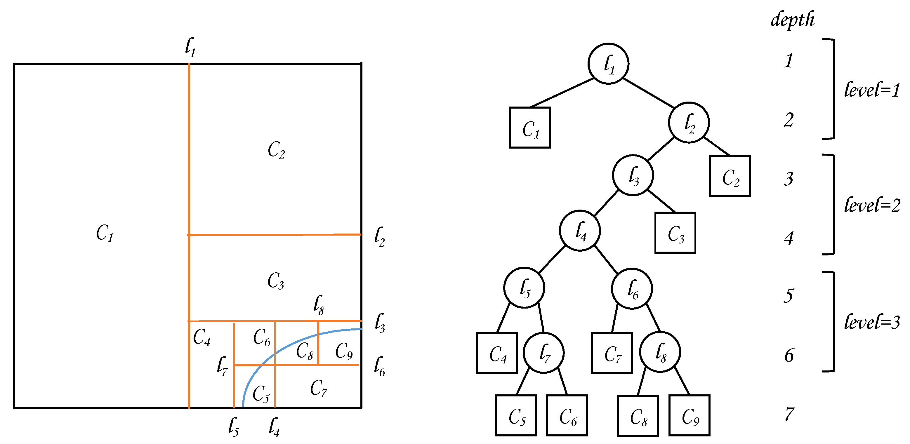
Figure 3.
Illustration of kd-tree based sub-division. The maximum level illustrated here is three. Each level consists of two depths that represent different splitting directions; (stored in nodes) and (stored in leaves) denote a splitting line and a sub-cell, respectively.
Figure 3.
Illustration of kd-tree based sub-division. The maximum level illustrated here is three. Each level consists of two depths that represent different splitting directions; (stored in nodes) and (stored in leaves) denote a splitting line and a sub-cell, respectively.
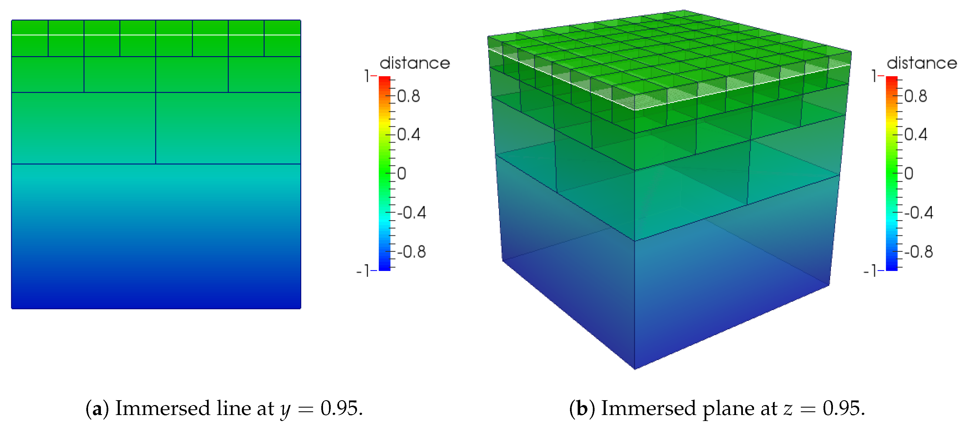
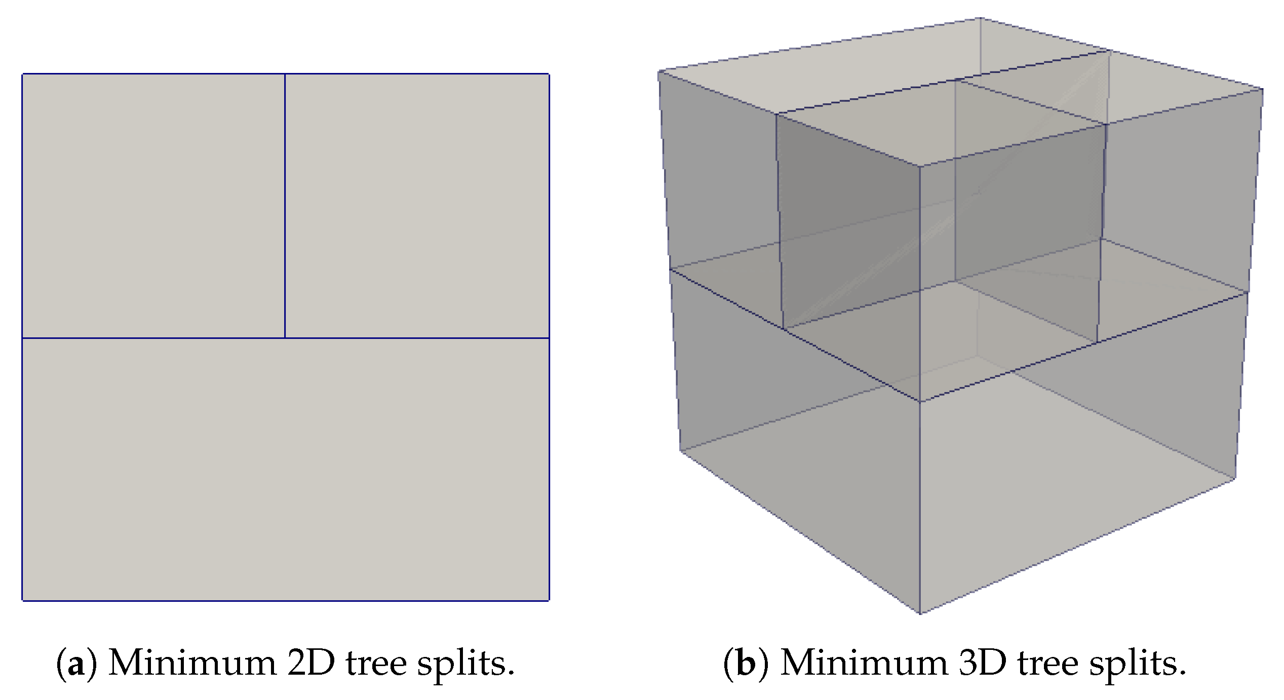
Figure 5.
kd-tree subdivision of a unit cell in the presence of (a) a 2D immersed line and (b) a 3D immersed plane. The maximum level is three in both examples. The domain color represents a signed distance to the immersed boundary.
Figure 5.
kd-tree subdivision of a unit cell in the presence of (a) a 2D immersed line and (b) a 3D immersed plane. The maximum level is three in both examples. The domain color represents a signed distance to the immersed boundary.
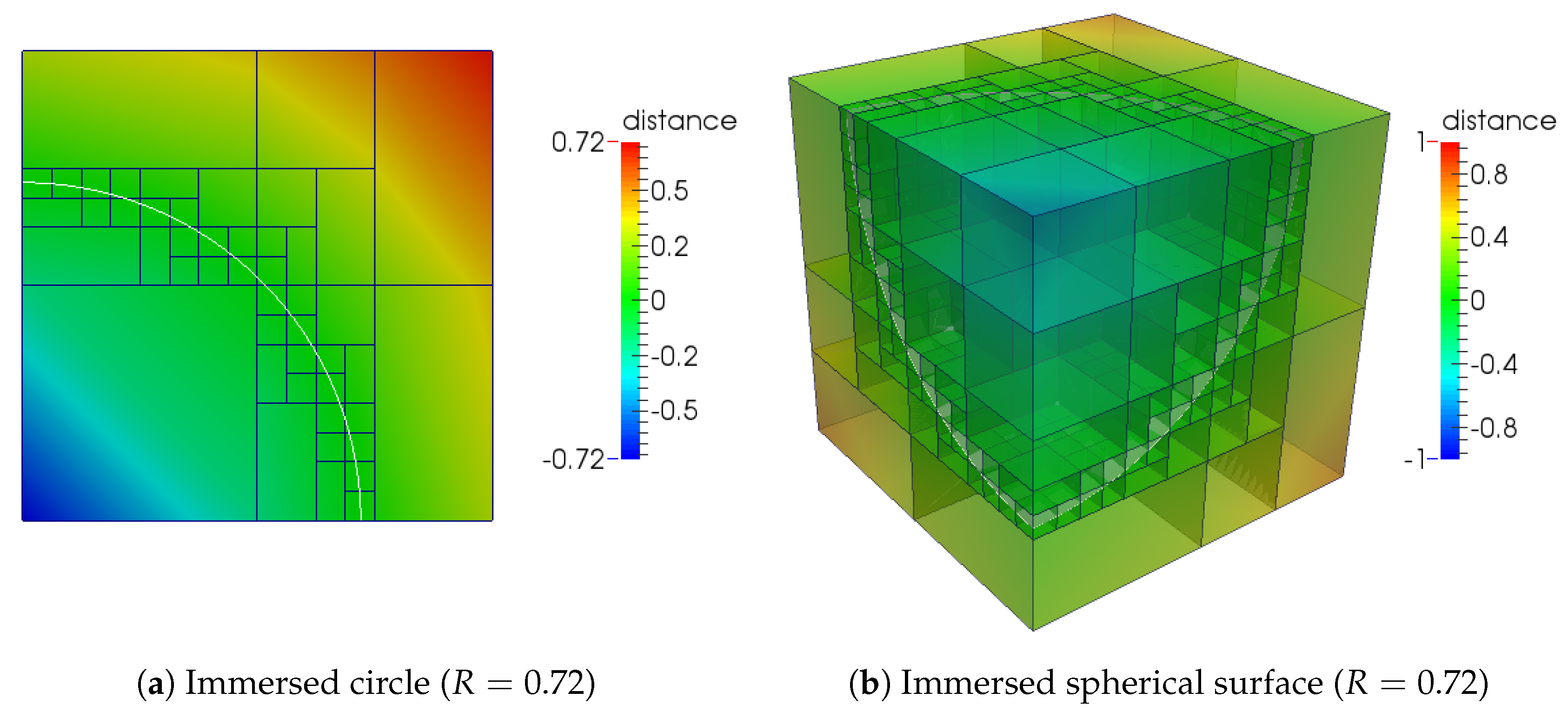
Figure 6.
kd-tree subdivision of a unit cell in the presence of (a) a quadrant and (b) a one-eighth spherical surface. The hyper-spheres are centered at a corner and have a radius of R. The maximum level is four in both examples. The domain color represents a signed distance to the immersed boundary.
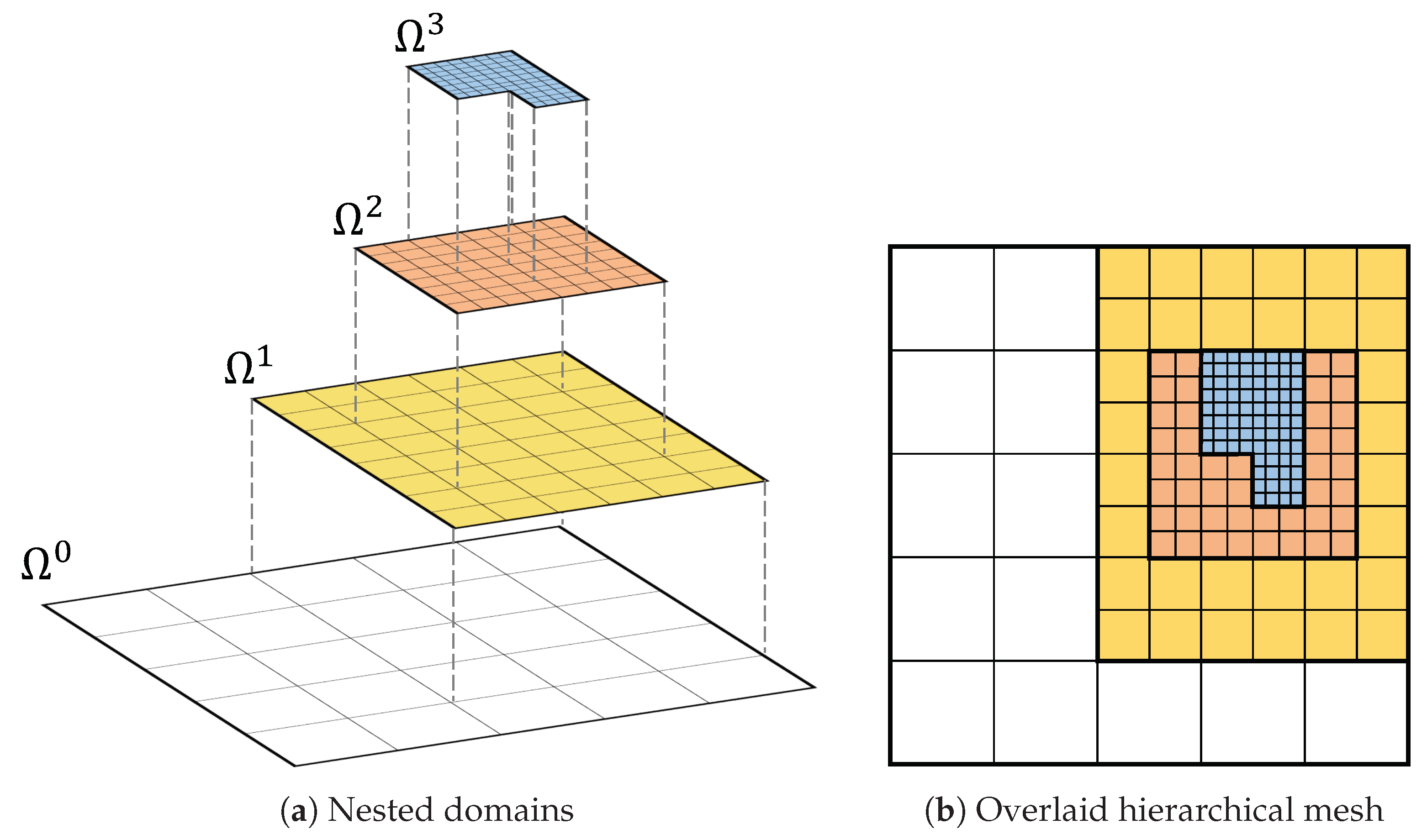
Figure 7.
A two-dimensional four-level dyadic hierarchical mesh: (a) the nested domains contain level-wise sub-meshes; (b) the sub-meshes are overlaid to generate the hierarchical mesh.
Figure 7.
A two-dimensional four-level dyadic hierarchical mesh: (a) the nested domains contain level-wise sub-meshes; (b) the sub-meshes are overlaid to generate the hierarchical mesh.
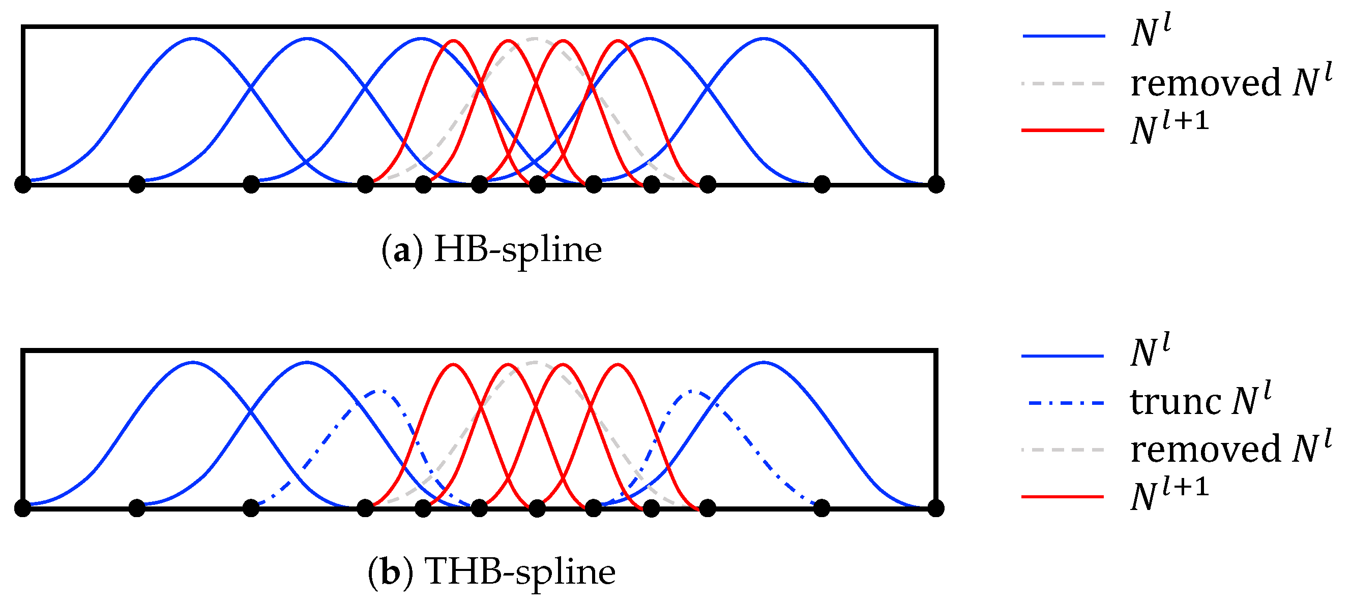
Figure 8.
Illustration of the basis functions of a two-level (a) hierarchical B-spline and (b) truncated hierarchical B-spline. The in the dashed line can be represented by a linear combination of , and is therefore removed to avoid linear dependence.
Figure 8.
Illustration of the basis functions of a two-level (a) hierarchical B-spline and (b) truncated hierarchical B-spline. The in the dashed line can be represented by a linear combination of , and is therefore removed to avoid linear dependence.
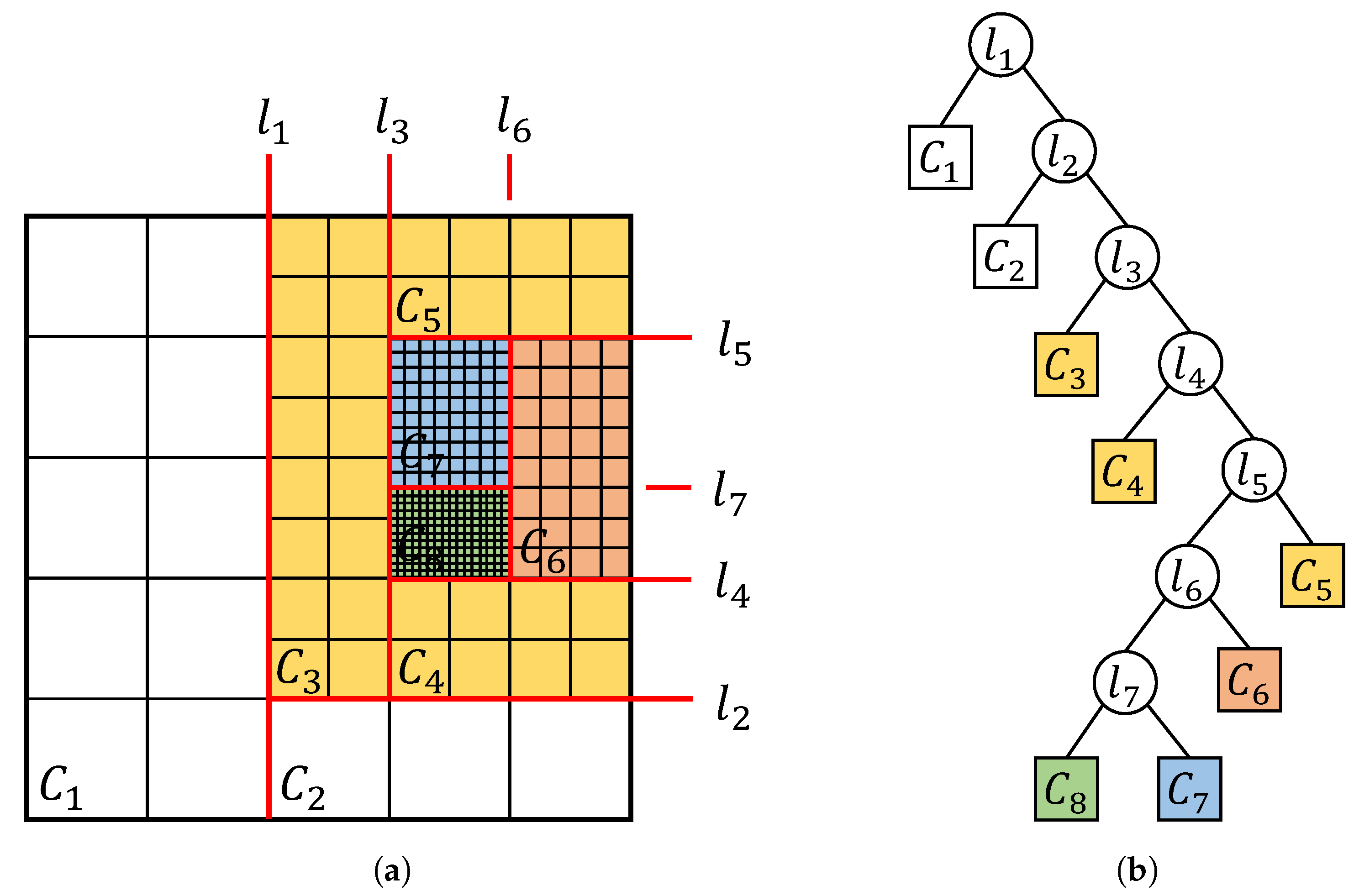
Figure 9.
kd-tree representation of a two-dimensional hierarchical mesh. (a) Splitting lines and cells in the hierarchical mesh; (b) kd-tree representation. In (a), the domain is subdivided into homogeneous cells, with each belonging to only one hierarchical level, while in (b) the splitting lines and the cells are stored in the internal nodes and leaves of a kd-tree data structure, respectively.
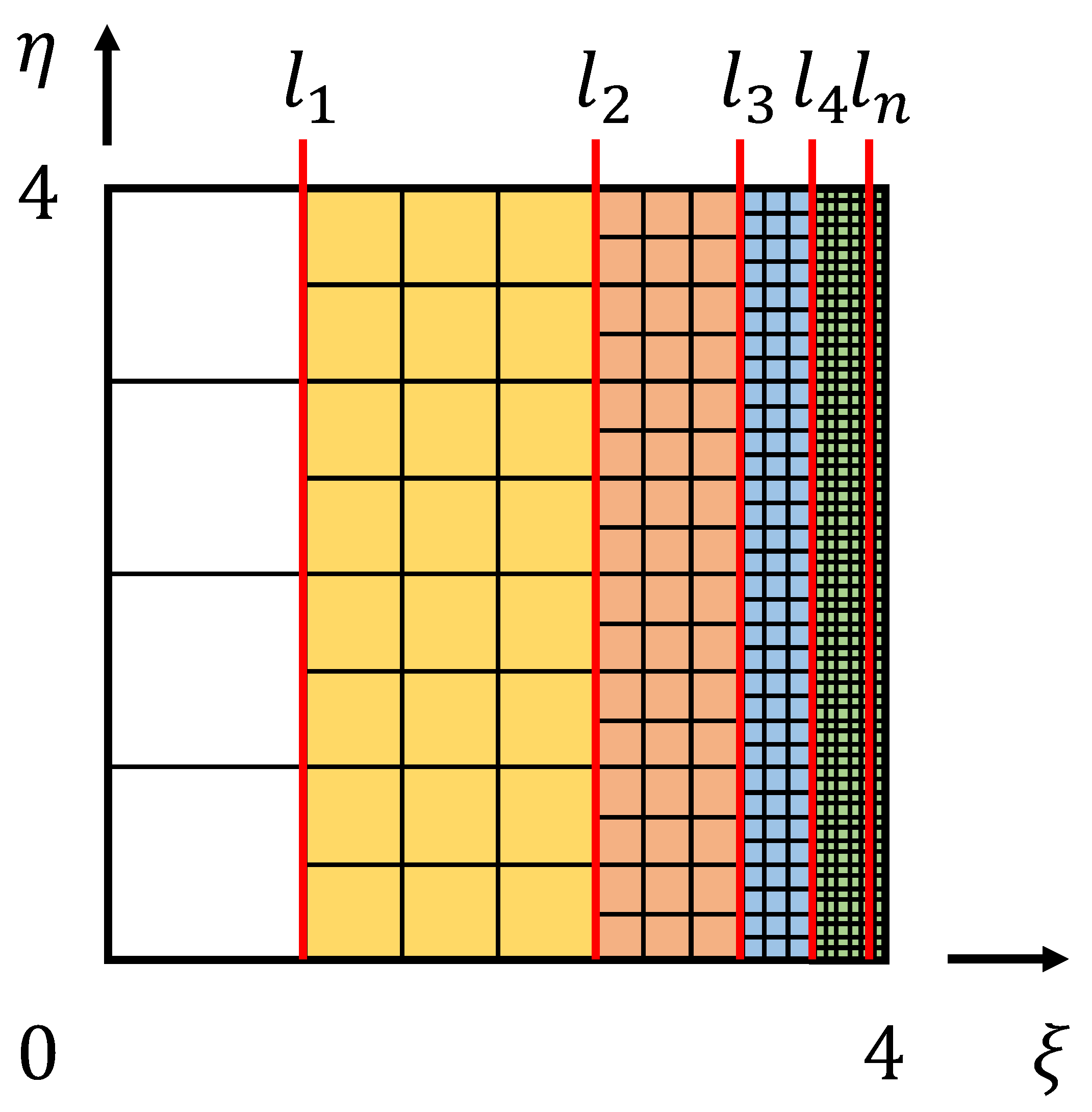
Figure 10.
n-stripe refinement on a domain. The left boundary of each refinement region is provided by and the right boundaries coincide at . The splitting lines during kd-tree subdivision are labeled with .
Figure 10.
n-stripe refinement on a domain. The left boundary of each refinement region is provided by and the right boundaries coincide at . The splitting lines during kd-tree subdivision are labeled with .
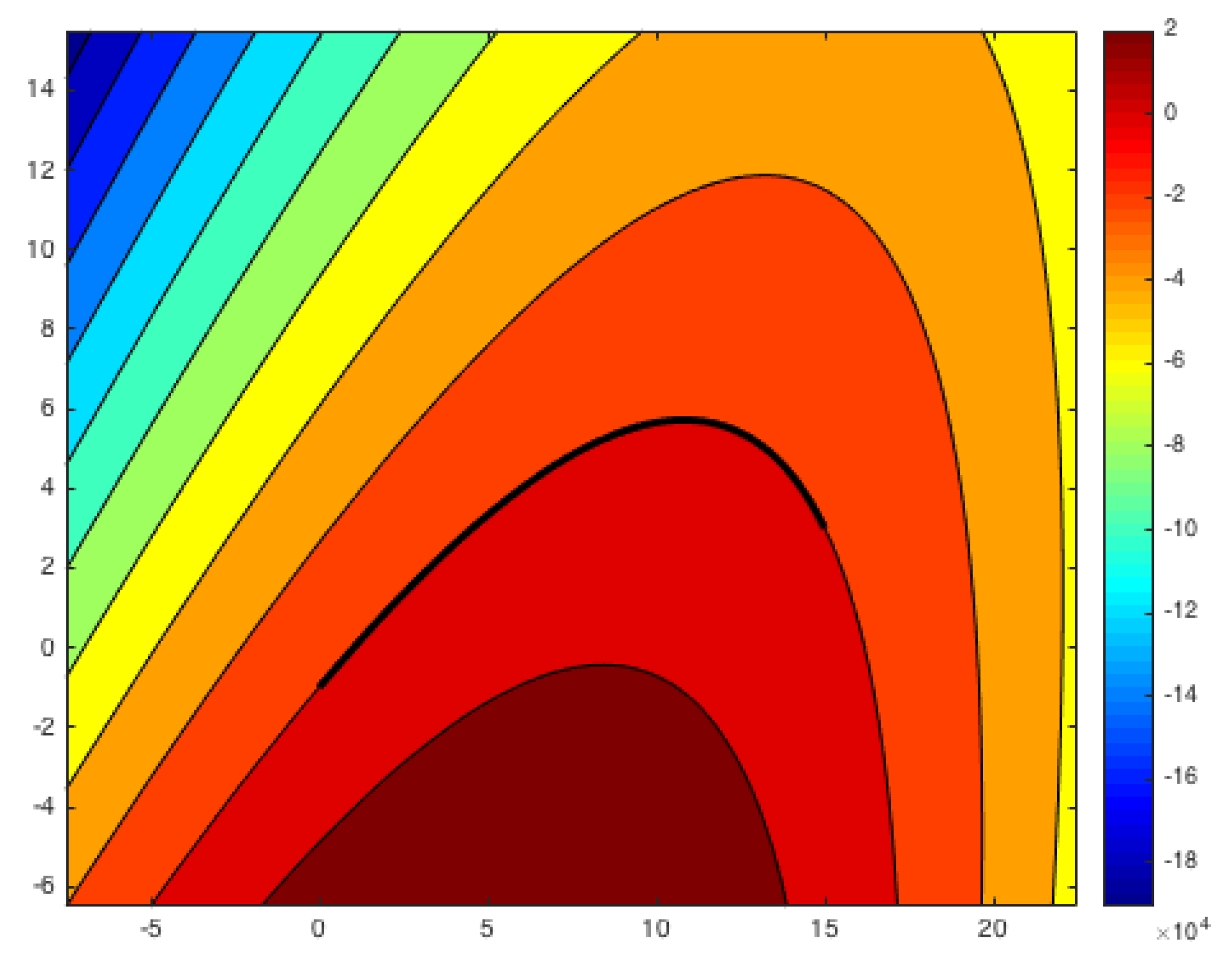
Figure 11.
Implicitization of a quadratic Bezier segment. Level set can be used as a measure of distance.
Figure 11.
Implicitization of a quadratic Bezier segment. Level set can be used as a measure of distance.
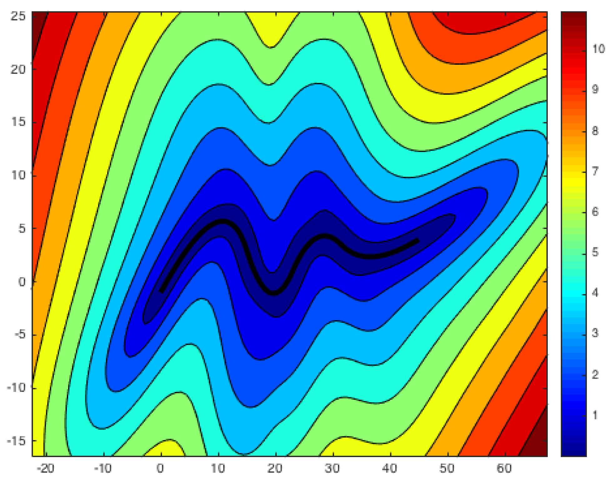
Figure 12.
Algebraic level sets from an open quadratic NURBS curve. The generated algebraic level sets ensure the smoothness of the field.
Figure 12.
Algebraic level sets from an open quadratic NURBS curve. The generated algebraic level sets ensure the smoothness of the field.
Figure 13.
Algebraic level sets from a closed quadratic NURBS curve.
Figure 13.
Algebraic level sets from a closed quadratic NURBS curve.
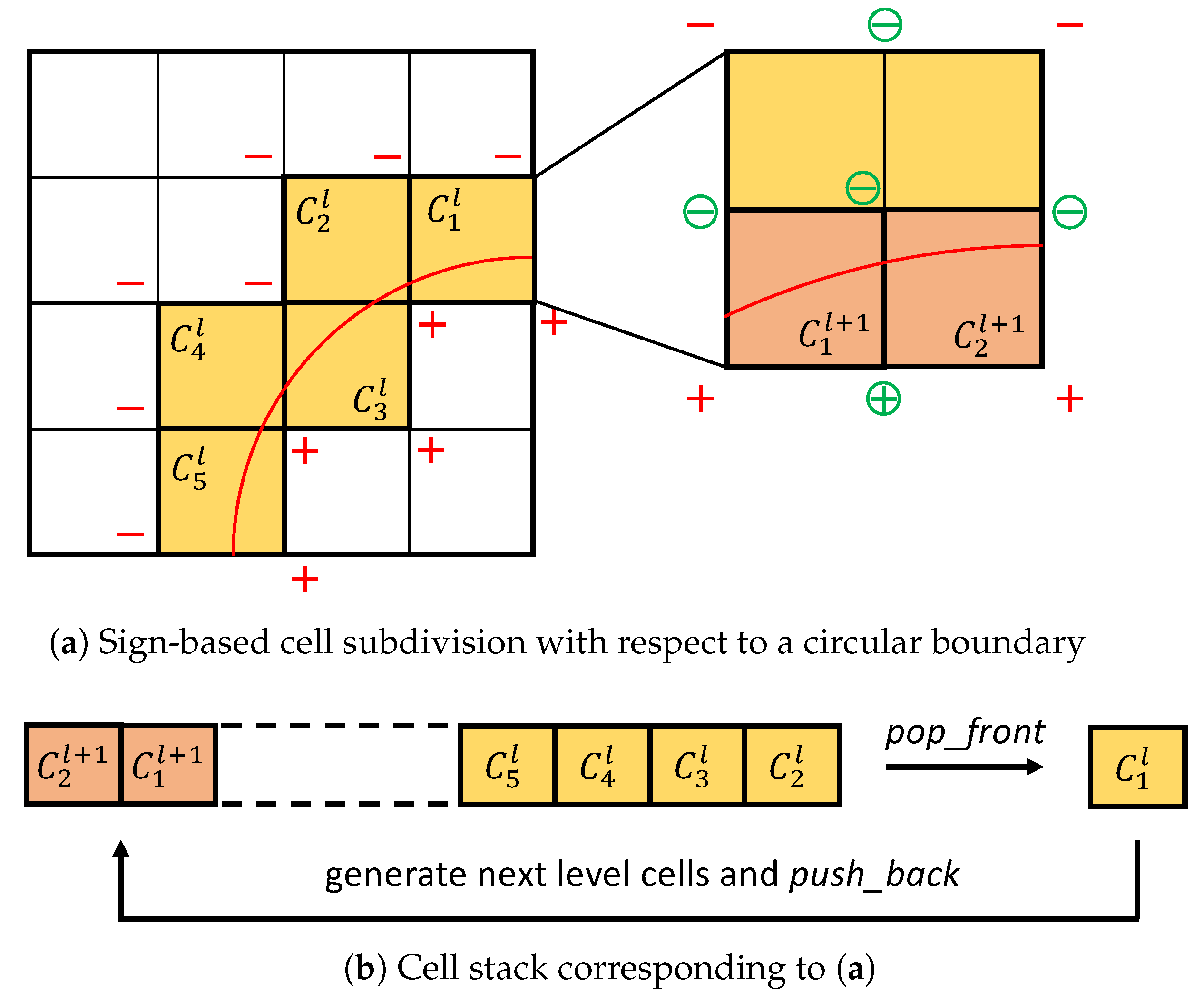
Figure 14.
Illustration of the sign-based refinement algorithm: (a) the cut cells in level l are subdivided into appropriate sub-cells. The new cut cells in level are identified by the newly calculated (circled) signs and the previously obtained (not circled) signs, and then (b) pushed to the back of the stack to wait for the next level subdivision.
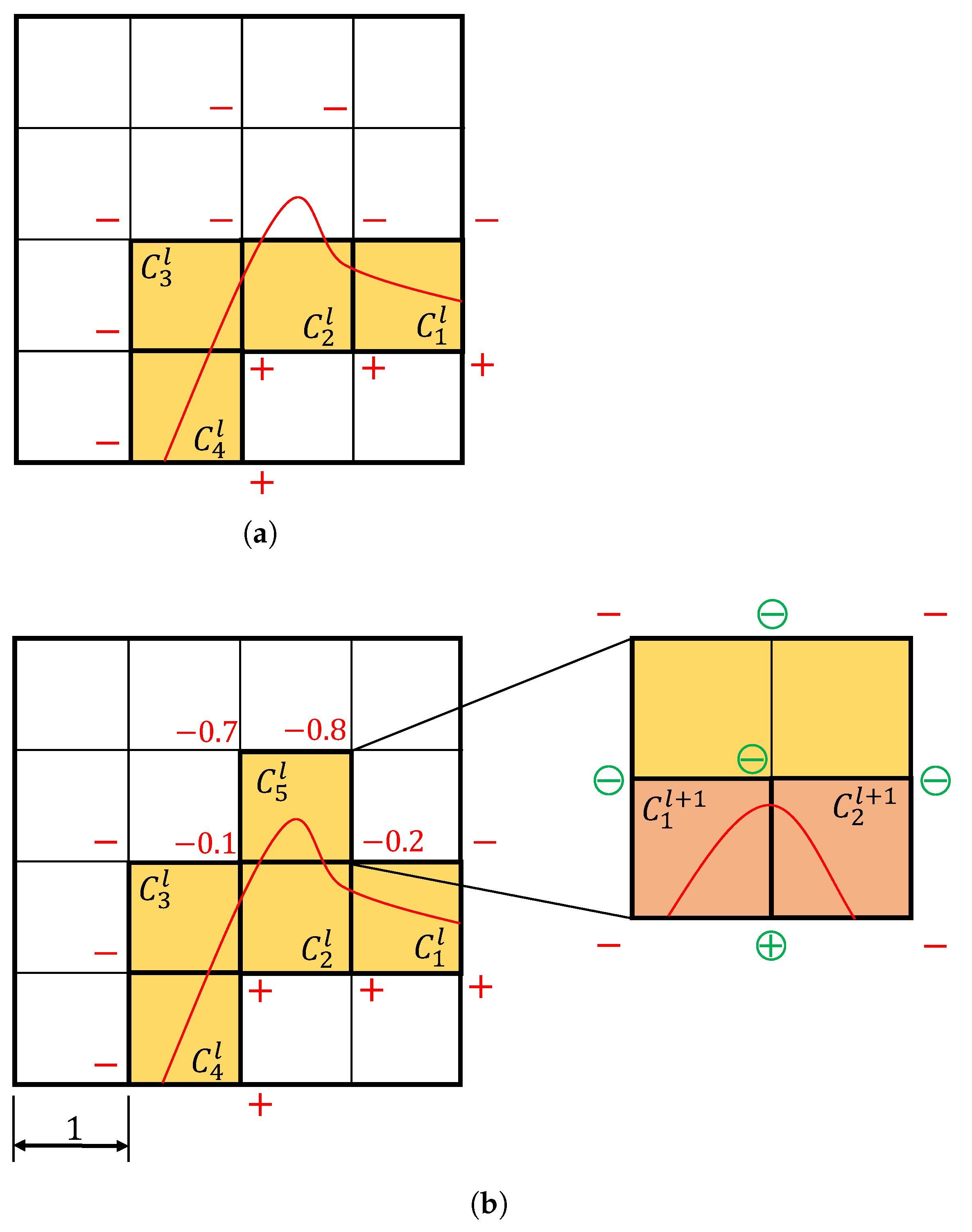
Figure 15.
(a) Determination of level l cut cells using the sign-based criterion. A cut cell is missed due to the small feature size. (b) Determination of level l cut cells using the distance-based criterion, followed by sign-based subdivision to generate the level cut cells. For a cell size , the distances of the vertices to the boundary are annotated in the figure.
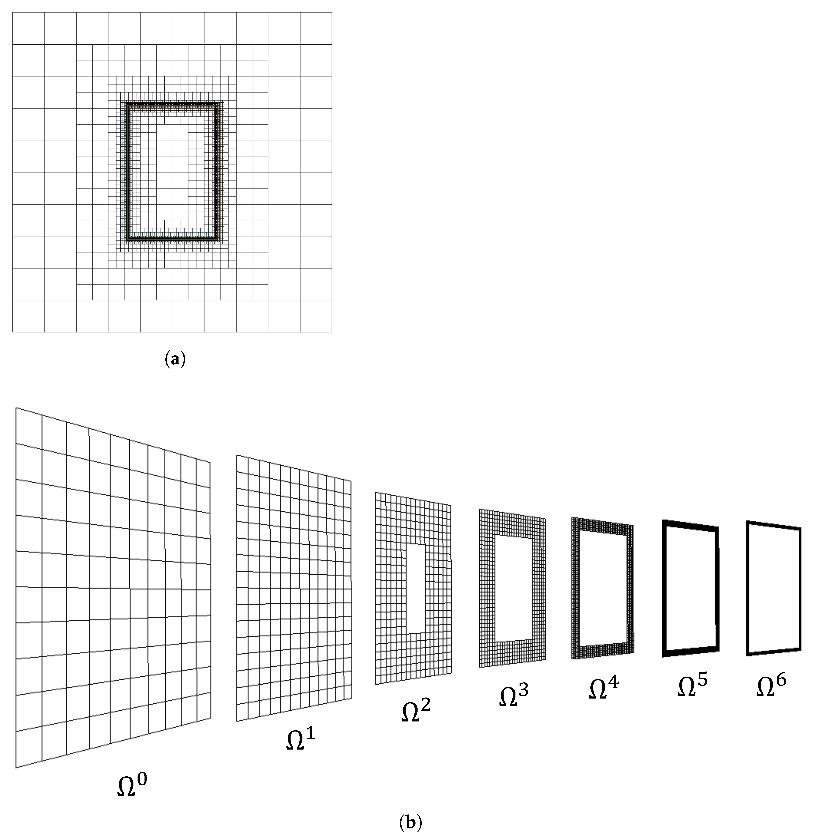
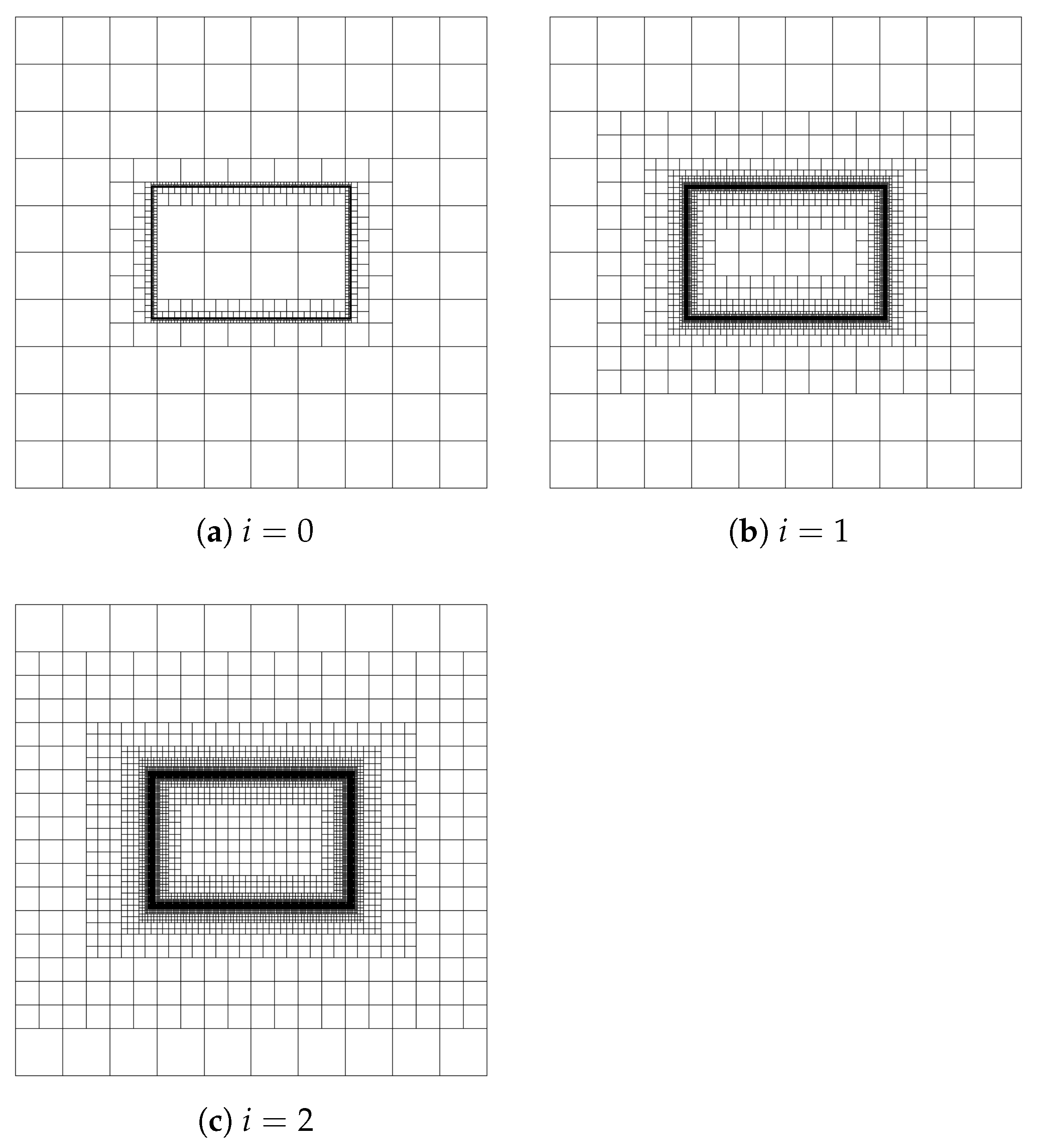
Figure 16.
A two-dimensional seven-level hierarchical refinement of a square domain with respect to a rectangular immersed boundary: (a) hierarchical mesh and (b) sub-meshes in each level.
Figure 16.
A two-dimensional seven-level hierarchical refinement of a square domain with respect to a rectangular immersed boundary: (a) hierarchical mesh and (b) sub-meshes in each level.
Figure 17.
Schematic of horizontal refinement: (a) the neighbors of a cut cell provide a larger refinement region, while (b) the union of the neighbors forms a refinement band.
Figure 17.
Schematic of horizontal refinement: (a) the neighbors of a cut cell provide a larger refinement region, while (b) the union of the neighbors forms a refinement band.
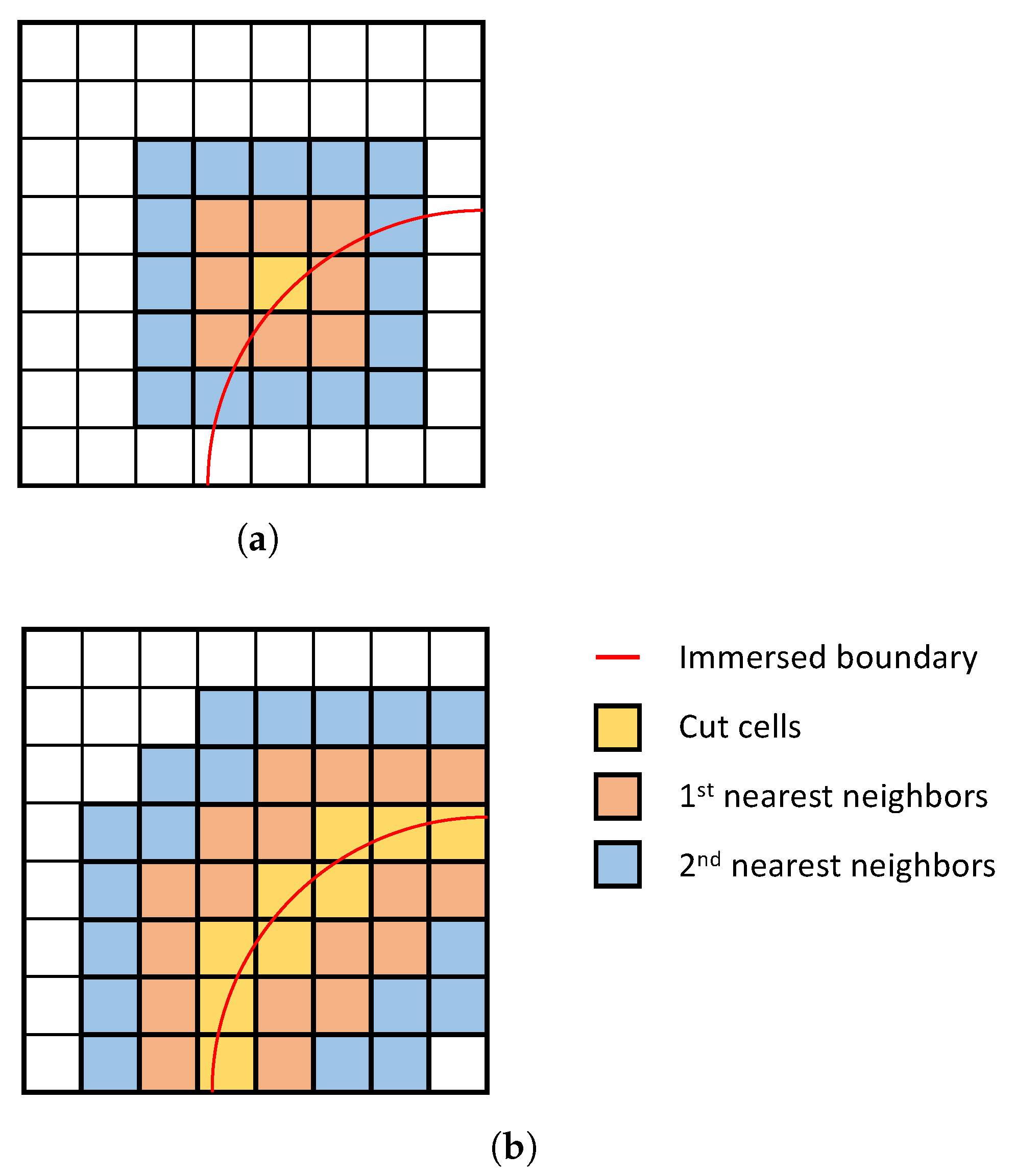
Figure 18.
Horizontal refinement with different bandwidth. (a) Only the cut cells are refined. (b) First-order refinement: the cut cells and their first nearest neighbors are refined. (c) Second-order refinement: the cut cells and up to their second nearest neighbors are refined.
Figure 18.
Horizontal refinement with different bandwidth. (a) Only the cut cells are refined. (b) First-order refinement: the cut cells and their first nearest neighbors are refined. (c) Second-order refinement: the cut cells and up to their second nearest neighbors are refined.
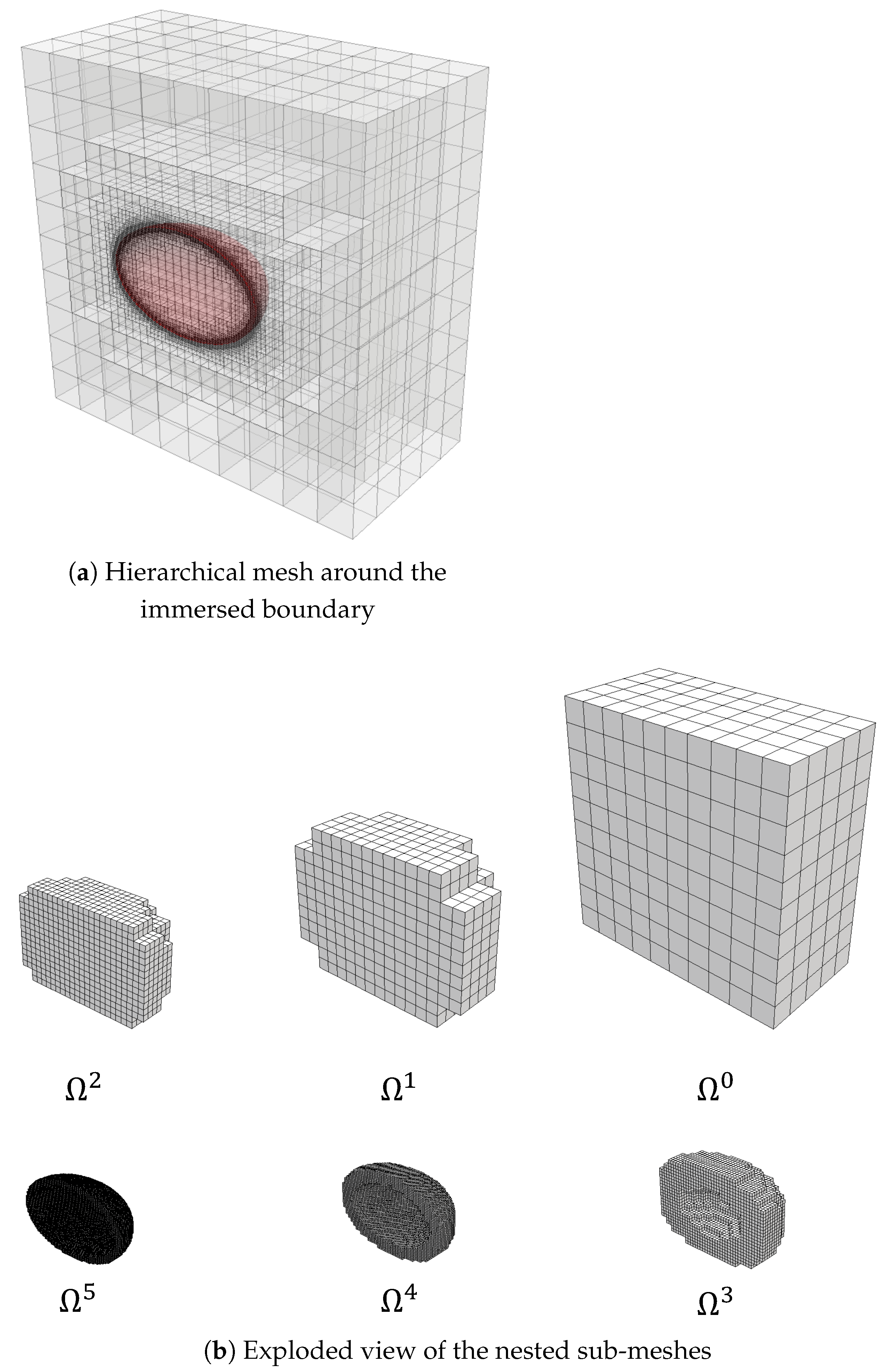
Figure 19.
A three-dimensional six-level hierarchical refinement of a cubic domain with respect to an ellipsoidal boundary: (a) hierarchical mesh and (b) sub-meshes in each level.
Figure 19.
A three-dimensional six-level hierarchical refinement of a cubic domain with respect to an ellipsoidal boundary: (a) hierarchical mesh and (b) sub-meshes in each level.
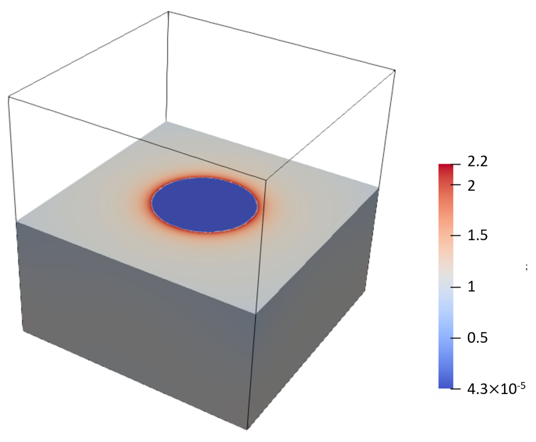
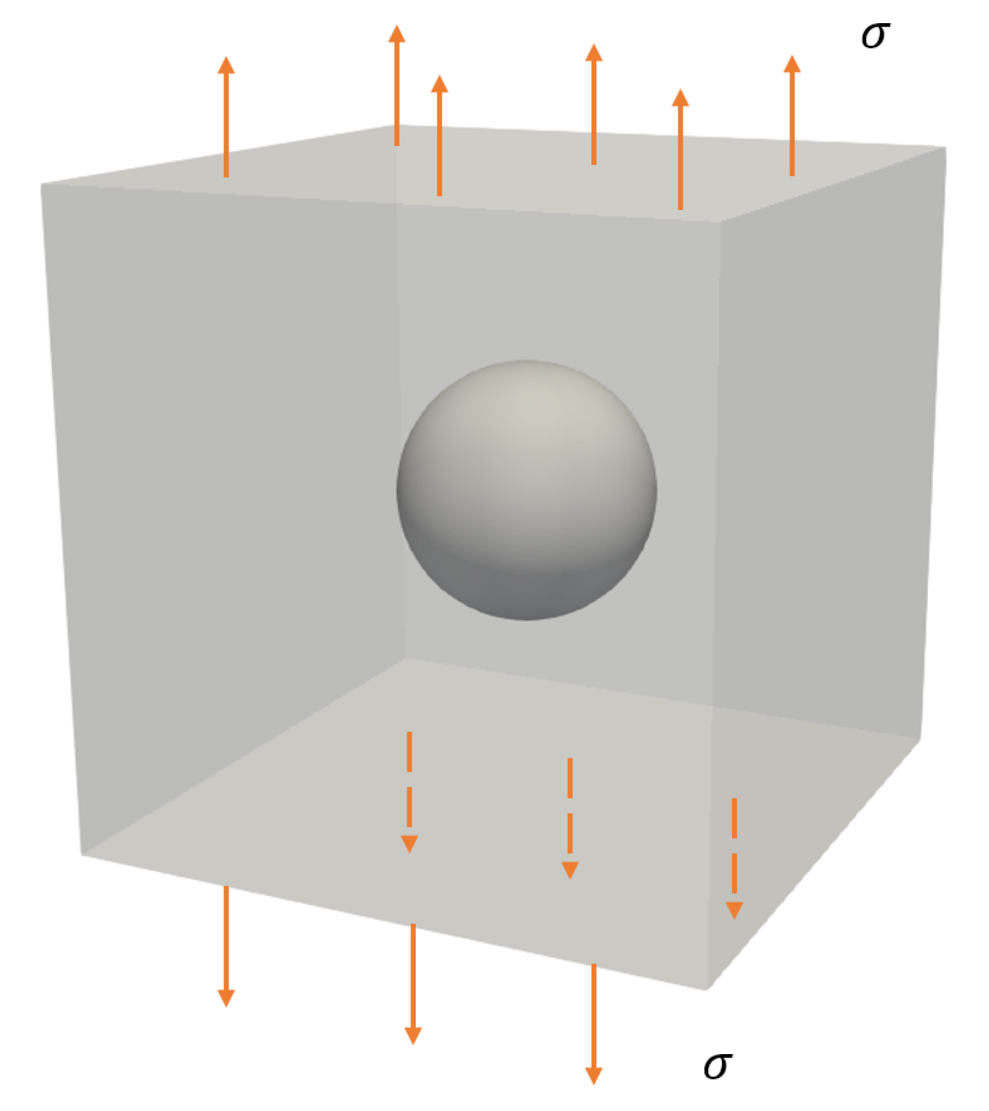
Figure 20.
Single spherical void under uniform fraction of unit magnitude.
Figure 20.
Single spherical void under uniform fraction of unit magnitude.
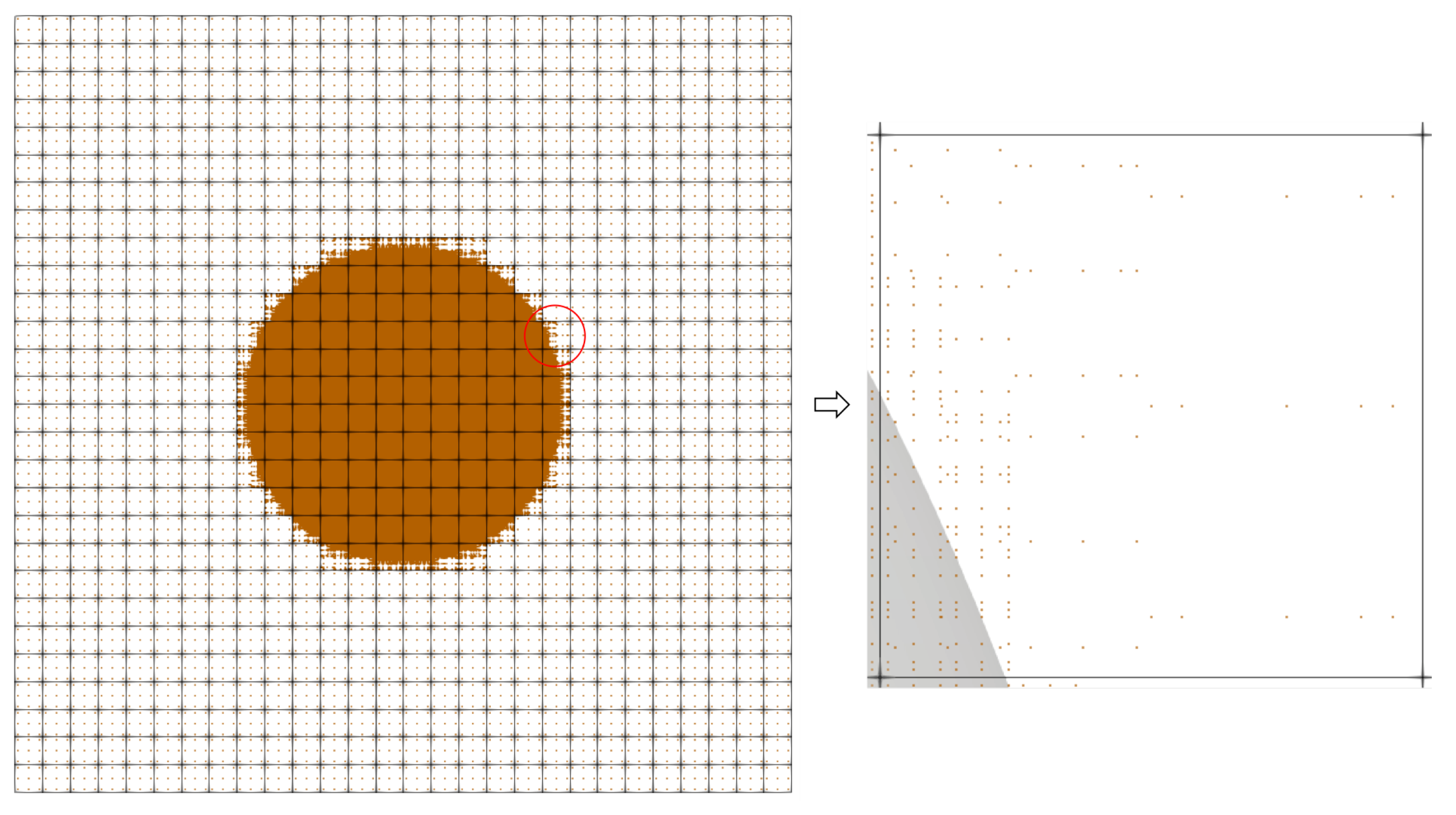
Figure 21.
Two-dimensional view (xy-plane) of quadrature points in the domain obtained using kd-tree cell division. A control point grid of was used.
Figure 21.
Two-dimensional view (xy-plane) of quadrature points in the domain obtained using kd-tree cell division. A control point grid of was used.
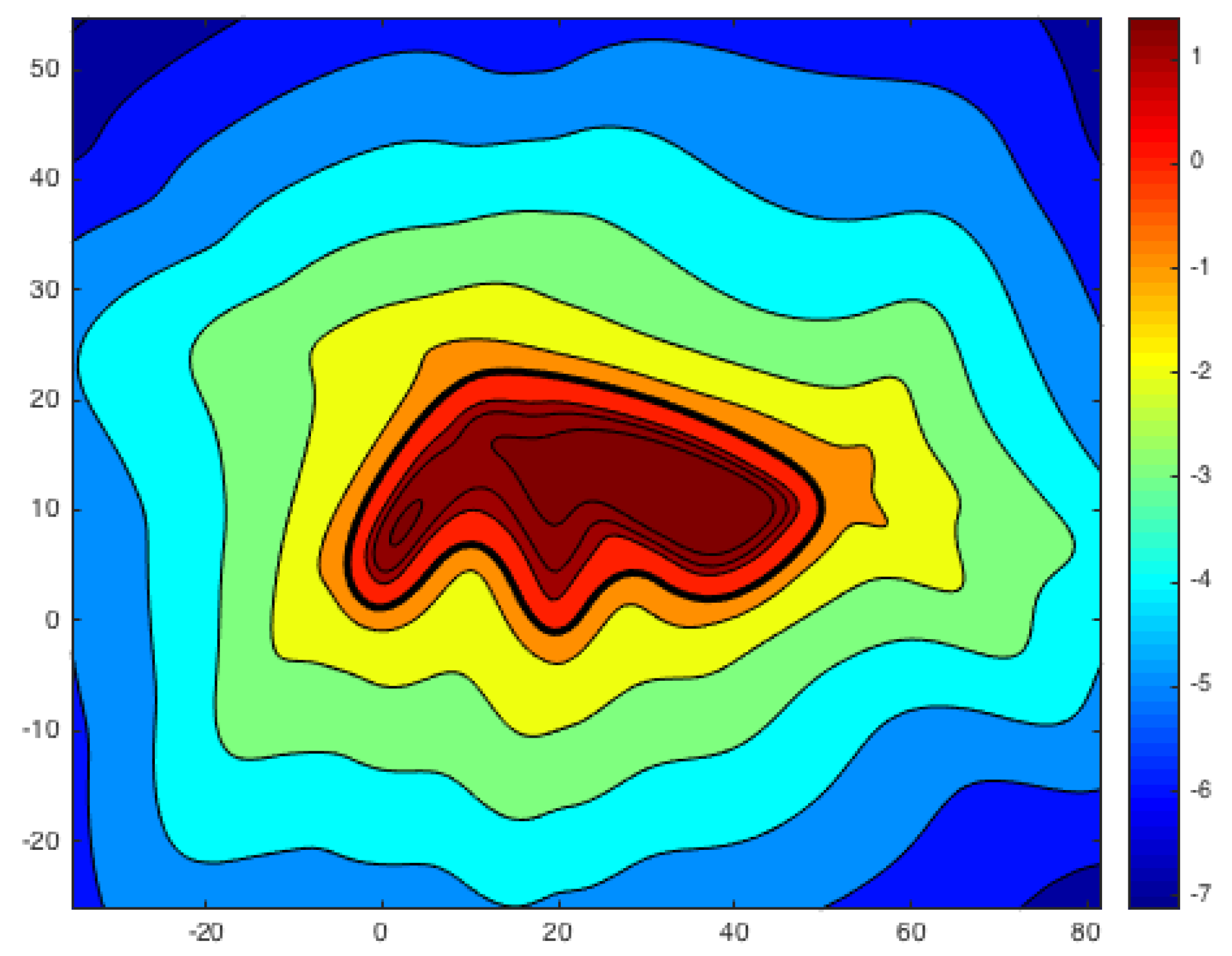
Figure 22.
Von Mises stress and stress concentration behavior around the equator of the spherical inclusion. The sphere has a diameter of and is placed at the center of a cubic domain.
Figure 22.
Von Mises stress and stress concentration behavior around the equator of the spherical inclusion. The sphere has a diameter of and is placed at the center of a cubic domain.
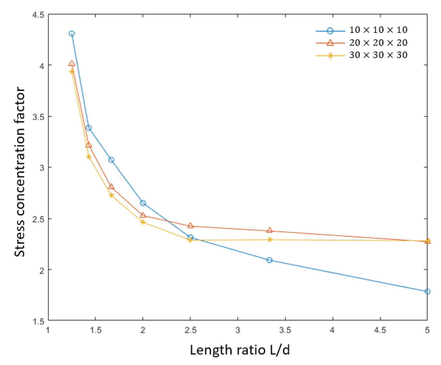
Figure 23.
Convergence of the stress concentration factor with refinement as a function of the scale ratio (where L is the size of the underlying cubic domain and d is the diameter of spherical void). The plots correspond to , , and control grids.
Figure 23.
Convergence of the stress concentration factor with refinement as a function of the scale ratio (where L is the size of the underlying cubic domain and d is the diameter of spherical void). The plots correspond to , , and control grids.
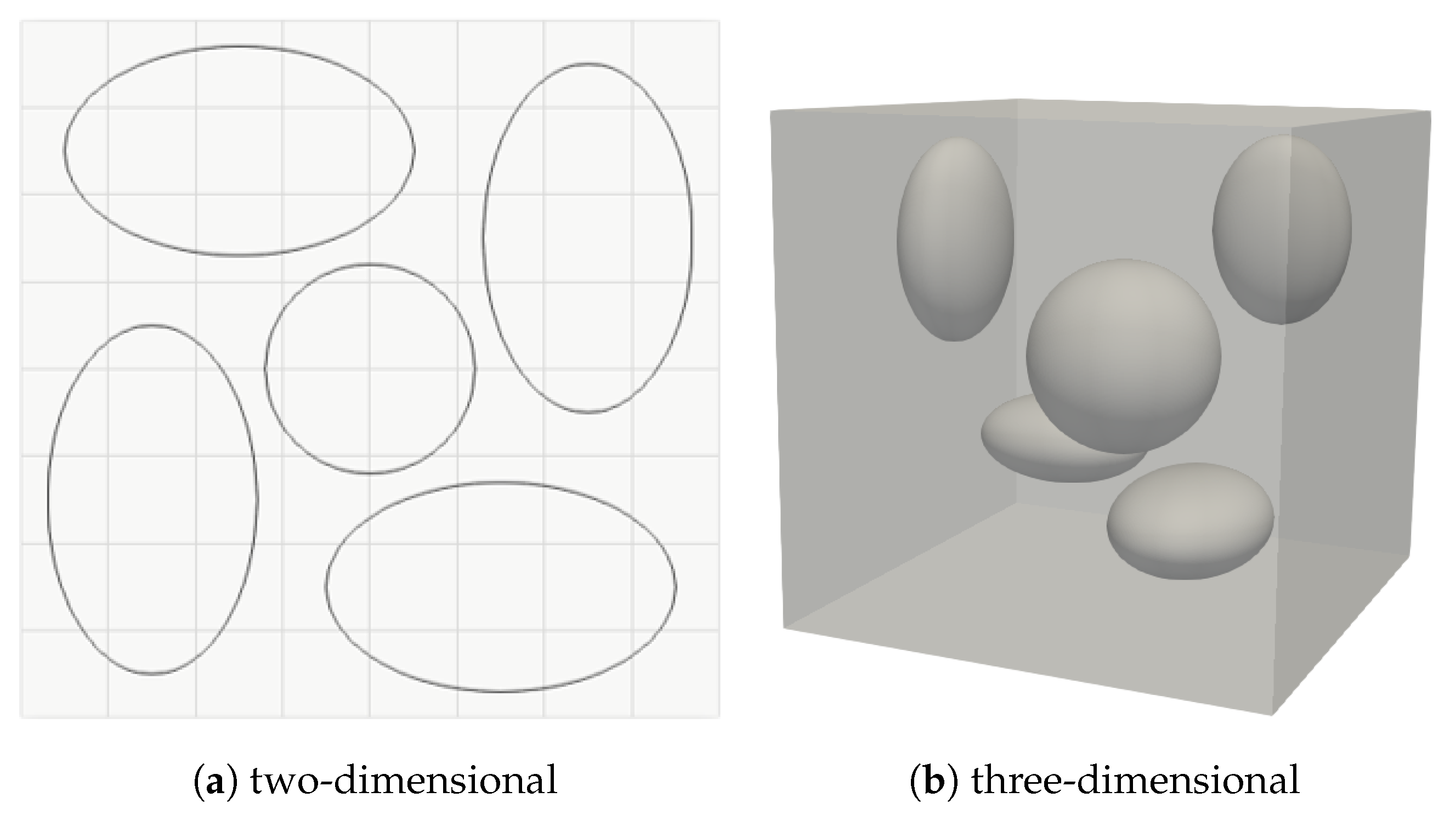
Figure 24.
Unit cell with five (a) elliptical and (b) ellipsoidal inclusions.
Figure 24.
Unit cell with five (a) elliptical and (b) ellipsoidal inclusions.
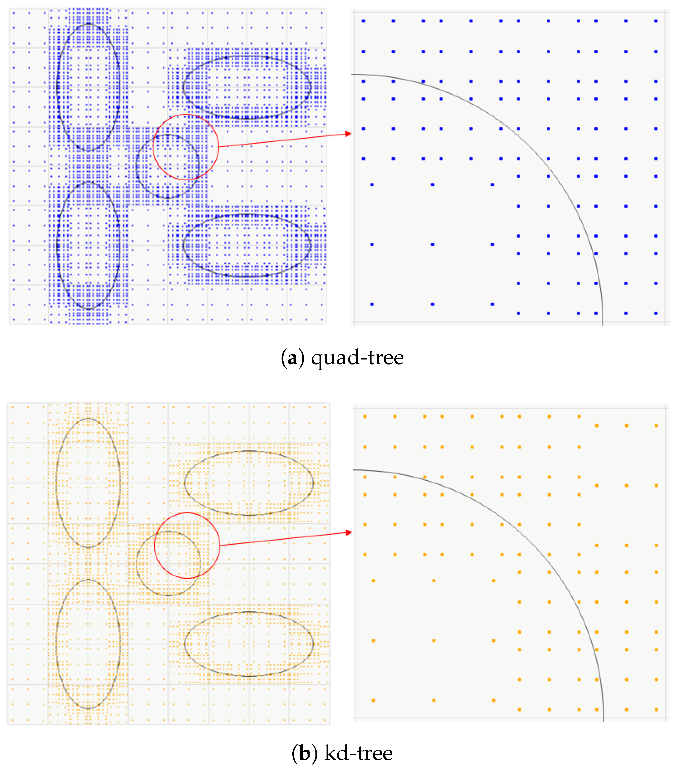
Figure 25.
Quadrature points generated for the example in
Figure 24a using (
a) quad-tree and (
b) kd-tree data structure with two sub-levels.
Figure 25.
Quadrature points generated for the example in
Figure 24a using (
a) quad-tree and (
b) kd-tree data structure with two sub-levels.
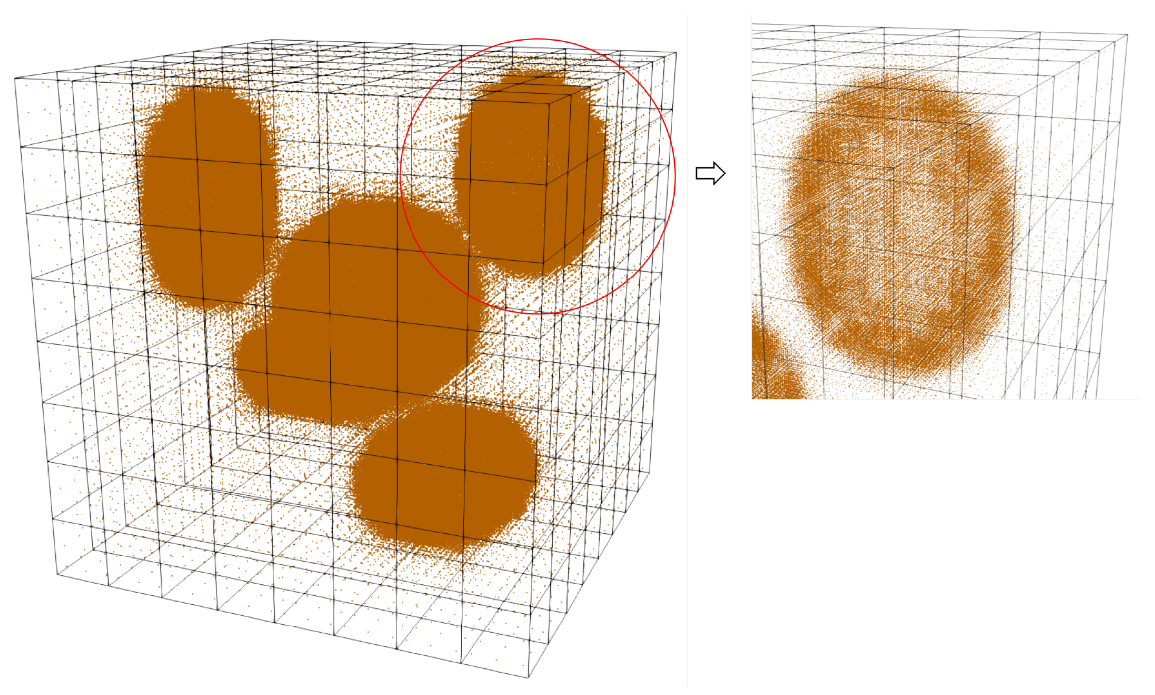
Figure 26.
Quadrature points generated for the example in
Figure 24b using a kd-tree data structure with two sub-levels.
Figure 26.
Quadrature points generated for the example in
Figure 24b using a kd-tree data structure with two sub-levels.
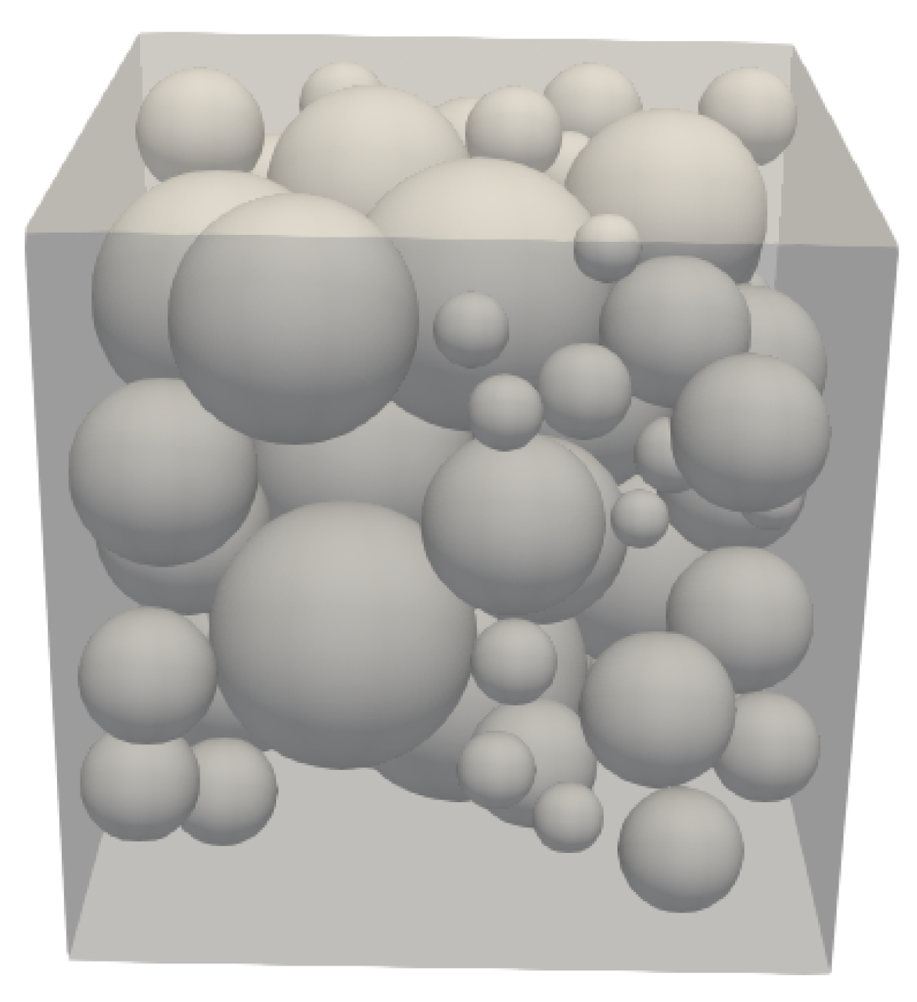
Figure 27.
Particulate system with 84 spherical fillers.
Figure 27.
Particulate system with 84 spherical fillers.
Table 2.
Aspect ratios of the sub-cells generated by quad-tree, oct-tree, and kd-tree subdivision. The initial element shape is assumed to be square (2D) or cubic (3D).
Table 2.
Aspect ratios of the sub-cells generated by quad-tree, oct-tree, and kd-tree subdivision. The initial element shape is assumed to be square (2D) or cubic (3D).
| Tree Type | Worst Case | Best Case |
|---|
| Quad-tree | 1:1 |
| Oct-tree | 1:1:1 |
| 2D tree | 1:2 | 1:1 |
| 3D tree | 1:1:2 | 1:1:1 |
Table 3.
Comparison of the kd-tree and quad/oct-tree subdivision in the presence of a hyper-planar boundary as shown in
Figure 5.
Table 3.
Comparison of the kd-tree and quad/oct-tree subdivision in the presence of a hyper-planar boundary as shown in
Figure 5.
| Tree Type | | Ratio of |
|---|
| 2D tree | 15 | 0.682 |
| Quad-tree | 22 | |
| 3D tree | 85 | 0.574 |
| Oct-tree | 148 | |
Table 4.
Comparison of kd-tree and quad/oct-tree subdivision in the presence of a hyper-spherical boundary as shown in
Figure 6.
Table 4.
Comparison of kd-tree and quad/oct-tree subdivision in the presence of a hyper-spherical boundary as shown in
Figure 6.
| Tree Type | | Ratio of |
|---|
| 2D tree | 48 | 0.787 |
| Quad-tree | 61 | |
| 3D tree | 521 | 0.722 |
| Oct-tree | 722 | |
Table 5.
Computer time on a personal computer required for hierarchical refinement of the geometry shown in
Figure 16.
Table 5.
Computer time on a personal computer required for hierarchical refinement of the geometry shown in
Figure 16.
| Number of Levels | 1 | 2 | 3 | 4 | 5 | 6 | 7 |
| Time Cost (−s)
| 0.1 | 0.7 | 1.4 | 3.2 | 6.8 | 14.8 | 36.7 |
Table 6.
Computer time on a personal computer required for hierarchical refinement of the geometry shown in
Figure 19.
Table 6.
Computer time on a personal computer required for hierarchical refinement of the geometry shown in
Figure 19.
| Number of Levels | 1 | 2 | 3 | 4 | 5 | 6 |
| Time Cost (−s)
| 0.1 | 2.4 | 8.6 | 47.9 | 166.3 | 434.8 |
Table 7.
Maximum von Mises stress (near equator) with different size of inclusion (
control points) in
Figure 23.
Table 7.
Maximum von Mises stress (near equator) with different size of inclusion (
control points) in
Figure 23.
| Diameter of Inclusion d | 0.8
| 0.7
| 0.6
| 0.5
| 0.4
| 0.3
| 0.2
|
| Length Ratio | 1.25 | 1.43 | 1.67 | 2 | 2.5 | 3.3 | 5 |
| Stress Concentration Factor | 3.93 | 3.10 | 2.72 | 2.46 | 2.29 | 2.29 | 2.28 |
Table 8.
Comparison of kd-tree and quad-tree cell division for quadrature cell refinement in the presence of multiple inclusions with elliptical boundary (shown in
Figure 24a).
Table 8.
Comparison of kd-tree and quad-tree cell division for quadrature cell refinement in the presence of multiple inclusions with elliptical boundary (shown in
Figure 24a).
| Tree Type | | Ratio of | | | Error |
|---|
| 2D tree | 3276 | 0.771 | 0.7173 | 0.7160 | |
| Quad-tree | 4032 | 0.7160 | |
Table 9.
Comparison of kd-tree and oct-tree cell division for quadrature cell refinement in the presence of multiple inclusions with hyper-spherical boundary (shown in
Figure 24b).
Table 9.
Comparison of kd-tree and oct-tree cell division for quadrature cell refinement in the presence of multiple inclusions with hyper-spherical boundary (shown in
Figure 24b).
| Tree Type | | Ratio of | | | Error |
|---|
| 3D tree | 118,476 | 0.735 | 0.9162 | 0.9618 | |
| Oct-tree | 161,244 | 0.9618 | |
Table 10.
Comparison of kd-tree and oct-tree cell division for quadrature cell refinement in a particulate system with 84 spherical fillers.
Table 10.
Comparison of kd-tree and oct-tree cell division for quadrature cell refinement in a particulate system with 84 spherical fillers.
| Tree Type | | Ratio of | | | Error |
|---|
| 3D tree | 15,753,744 | 0.740 | 0.4256 | 0.4256 | |
| Oct-tree | 21,287,043 | 0.4256 | |


