Topic Modeling for Automatic Analysis of Natural Language: A Case Study in an Italian Customer Support Center

Abstract

This paper focuses on the automatic analysis of conversation transcriptions in the call center of a customer care service. The goal is to recognize topics related to problems and complaints discussed in several dialogues between customers and agents. Our study aims to implement a framework able to automatically cluster conversation transcriptions into cohesive and well-separated groups based on the content of the data. The framework can alleviate the analyst selecting proper values for the analysis and the clustering processes. To pursue this goal, we consider a probabilistic model based on the latent Dirichlet allocation, which associates transcriptions with a mixture of topics in different proportions. A case study consisting of transcriptions in the Italian natural language, and collected in a customer support center of an energy supplier, is considered in the paper. Performance comparison of different inference techniques is discussed using the case study. The experimental results demonstrate the approach’s efficacy in clustering Italian conversation transcriptions. It also results in a practical tool to simplify the analytic process and off-load the parameter tuning from the end-user. According to recent works in the literature, this paper may be valuable for introducing latent Dirichlet allocation approaches in topic modeling for the Italian natural language.

1. Introduction

In computer science, natural language processing (NLP) is a research domain that deals with semantic mining, enabling computers to obtain meaning from human language [1]. Topic modeling (TM) is an area of research for the scientific community of NPL.

Generally, NLP includes machine translation, content extraction, question answering, information retrieval, and text generation [2]. Furthermore, NLP includes text classification, the grouping of documents based on similar characteristics and contents, concepts/topics detection and extraction, sentiment analysis, and text summarization. TM is a text mining approach to address the problem of grouping documents based on their topic and similarities by automatically finding patterns and characteristics from the data itself without any predefined data labels. With its capability, TM enables understanding of the collection of documents as well as the building of a robust search engine [3].

TM finds hidden subjects in the collection and describes the relationships between them and each document. TM clusters the documents and indicates the contents of each cluster simultaneously. Several practical TM techniques were proposed in previous research, including probabilistic latent semantic analysis (PLSA) [4], non-negative matrix factorization (NMF) [5], latent Dirichlet allocation (LDA) [6] and structural topic modeling (STM) [7]. In recent years, the studies on the application of TM methods were also active, for example, in political science, bio-informatic, healthcare, and medicine [7,8,9,10,11].

In a customer support center, the LDA algorithm enables the modeling, of conversation transcriptions, between customers and agents, as topical mixtures. Each topic is a multinomial distribution over problems and complaints discussed in the conversation. LDA interprets each transcription as an unordered bag-of-words, and a transcription is a probabilistic realization of a mixture model over customer problems and complaints. Through the LDA algorithm, the analysis of transcriptions can provide insights into the quality of the service. “Perplexity” is an example of a metric that allows accurate evaluation of LDA results and the model generalization ability likelihood on unknown data [12,13].

Besides the used approach to analyze the text documents, given the amount of data available, making the mining activity automatic is the natural requirement of any actual application. The possible constant use of the human control of the activities would involve not fully exploiting the potentialities of the mining techniques. Text mining is a multi-step process that requires specific configurations and the choice of parameters for each step of the analysis. Hence, some kind of expertise is required to guide the analysis process. Solutions for investigating a large set of transcriptions, without supervision by human analysts and data experts, may be of practical value in real applications.

Until now, most of the representative text pre-processing tools and language models have been based on English. Thus, the majority of data sources used in text-based research are also documented in English. Current NLP methods and algorithms mainly focus on several high-resource languages, such as English, Chinese, Japanese, Korean, German and French. Low-resource languages, such as Italian, were underserved by NLP systems. That is mainly due to the lack of datasets and support for the specific language. Furthermore, English approaches cannot be extended to other languages because the dictionary is not the same, and each language requires its own lexicon database [14]. There are several crucial challenges in the multi-lingual and cross-lingual development of NLP models [1]. Therefore, it is essential to develop research projects at the country level to create NLP applications for domestic languages. An example related to a low-resource language, such as the Persian natural language, can be found in [15]. Similar to recent advances in the literature [16,17], the present study aims to contribute to the literature by developing an NLP application, specifically a TM algorithm, for the Italian natural language.

In this research, we develop a framework that automatically clusters dialog transcriptions into groups based on the content of the data. We use an LDA algorithm and discuss a method for determining the number of topics in a set of actual transcriptions in the Italian natural language. Dialogues between agents and customers in a customer support center define the reference case study. After introducing and implementing the framework, some experiments are illustrated to compare different fitting methods of the LDA algorithm. A quantitative performance measure is used to evaluate the effectiveness of the produced LDA solution for each fitting method considered in our comparison study.

This paper is structured as follows. Section 2 elaborates on the research field concerning TM. Section 3 provides theoretical foundations on the LDA algorithm and the metric for performance evaluation. Section 4 describes the functioning of text pre-processing, focusing on the Italian natural language. Section 5 is devoted to the actual application and problems addressed in the study. Section 5 also summarizes some results of the case study. Finally, Section 6 provides the conclusion and suggestions for future studies. The following two subsections provide the motivation example of our research, and the related work in the literature on fitting methods for the LDA algorithm.

1.1. Motivation Example

Human-to-human spoken dialogue analysis is becoming more popular in the literature. Advances in this research area are described in [18]. Topic identification, for which a state-of-the-art review is in [19], represents the basic component of the present study. The application considered in this paper deals with the automatic analysis of dialogues between a call center agent who can solve problems defined by the application domain documentation and a customer whose behavior is unpredictable [20].

Real-world human-to-human telephone calls, in which an agent asks a customer to formulate an issue and then attempts to solve it, are considered. The customer is expected to seek information or formulate complaints about the energy supplier system and services. The issues in this domain application can be summarized as follows: First, real-world customers have an unpredictable language style. Second, there is a verbose nature in conversations in a customer support center. Customers frequently describe their problems in factual terms, while agents use a broad introduction followed by a concise formal explanation that includes theme-specific terminology and phrases. Finally, the conversations are in the Italian natural language only, which is rarely considered in the literature on NPL approaches.

The objective is to investigate a customer problem over some time. Survey data are used to create problem percentages to track user satisfaction and prioritize problem-solving initiatives. TM is essential for assembling precise reports that can be used to conduct a reliable survey. A computerized system was put in place, with a voice recognition module for obtaining automatic transcriptions of the discussions. The main challenges are as follows: One or more subjects may be discussed in the conversations to be examined. Valuable issues may be interspersed with irrelevant comments. Mentions might be incomplete or erroneous due to repetition, ambiguity, and language and pronunciation errors. Discussions about an application-related issue may become irrelevant in some cases.

1.2. Related Work

LDA [6] is a Bayesian model for extracting latent semantic topics from text. It can be considered as the categorical/discrete analog of principal component analysis (PCA) to extract latent aspects from collections of discrete data. In LDA, the required posterior distribution is intractable, and hence it is not possible to apply exact inference to calculate it. Therefore, approximate inference techniques are usually employed. For the text topic modeling in our case study, where there is a large topic overlap that makes a difficult inference, we consider both variational Bayes (VB) and collapsed Gibbs sampling (CGS) techniques.

VB techniques, which are the original inference technique used in LDA [6], is a family of optimization-based techniques for approximate Bayesian inference. VB belongs to the class of variational inference (VI) methods, which can also be used in the frequentist context for maximum likelihood estimation when there are missing data.

VI inference techniques directly optimize the accuracy of an approximate posterior distribution. This is parameterized by free variational parameters [21]. In VI, we choose a family of distributions and then we find the member of this family (by finding the setting of the parameters) for which a divergence measure is minimized. In practice, the inference problem is translated into an optimization problem and solved with the standard expectation–maximization (EM) algorithm [21,22]. The EM performs two steps: the E-step, which estimates the topic distribution of each training document using current model parameters, and the M-step, which updates the model parameters. The success of VB as approximate inference strategies for LDA has resulted in their widespread use for TM by practitioners [23]. Two of the main Python implementations are Scikit-learn [24] and Gensim [25]. However, when working with a large topic overlap, which complicates the inference, the quality of extracted aspects can be compromised since that variational EM can lead to inaccurate inferences and biased learning.

Griffiths and Steyvers in [26] presented the CGS technique, which is a Markov chain Monte Carlo procedure. Given that CGS is a straightforward approach and rapidly converges to known ground truth, it can be considered an alternative to VB approaches for many LDA variants. However, CGS may present the critical drawback of high computational complexity that makes it inefficient on large data sets. In [27], a method was further presented for improving the computational performance of CGS-based LDA while providing similar results of the original LDA algorithm.

In this article, the objective is to provide the reader with a comparison of different VB and CGS inference techniques used in LDA fitting. To this aim, we do not alter the LDA model, nor do we use document pooling or transfer learning, but instead we present a method that employs the full joint distributions arising from the standard LDA model.

2. Topic Modeling

The goal of TM is to define the topics within a data set of transcriptions, of which there is no a priori information; the output of TM is a set of clusters, that is, homogeneous groups of transcriptions that deal with the same topic. The models can be distinguished based on the ability to manage the presence of multiple themes within the transcription: some models handle these documents as outliers by excluding them from all the clusters formed; other models represent the co-presence as a probability distribution of more topics in the transcription. Within the reference case study of our study, it is not unusual to deal with multitopic conversation transcriptions between customers and agents and topics overlapping in the customers’ support requests.

The basic concept of TM methods is taking the numeric (document × term) vectors that represent the documents as input and converting them into (topic × term) vectors and (document × topic) vectors. Each input transcription is assigned to one topic group using the (document × topic) matrix.

How documents are represented numerically is one of the basic features of a TM method; in the bag-of-words paradigm, the most widely used approach, documents are a collection of unordered words. The “term frequency”–“inverse document frequency” is a widely-used technique for implementing a bag-of-words in TM by adding the importance of the term in the collection to the count vector.

The first component is the “term frequency”, which counts how many times each phrase appears in a document; the second component is the “inverse document frequency” which determines the extent to which a phrase is used throughout the text. However, using this representation, relationships between words are lost during text processing. To deal with this problem, in 2013, the research team at Google advocated a new approach, called Word2Vec [28], which involves two-layer neural networks and embeds each word in a numeric vector space. The technique allows the semantic similarity of words to be calculated, and a document can be characterized by a vector incorporating the relationship between the words using the average values of Word2Vec [29]. Such a technique was further developed and expanded to the document scale, which is called Doc2Vec [30].

Starting from the numerical representation in a vector space, TM methods can be categorized into two types of models: probabilistic and non-probabilistic. Examples of the first type of approach are the probabilistic latent semantic analysis (PLSA) [4] and the latent Dirichlet allocation (LDA) [6]. PLSA and LDA methods calculate the likelihood of a word appearing in several subjects, and the likelihood of the topics in the document. The non-negative matrix factorization (NMF) [5] and the latent semantic analysis (LSA) [31] are two non-probabilistic approaches. Both NMF and LSA are algebraic approaches using matrix factorization.

Among the number of methods proposed in the literature, LDA and NMF are the most popular techniques for actual applications [32,33,34]; at the same time, using various data sets, researchers continue to investigate improved TM algorithms. Studies in [35,36,37] were conducted to compare the existing techniques explained above, and the conclusions show that the best methods are different depending on the data sets.

Improvements in the LDA performance are provided by the embedded topic model (ETM), presented in [38]. The ETM is a document model that matches the original LDA to find an interpretable latent semantic format for the documents, and word embeddings to provide a low-dimensional representation of the meaning of words. For the present study, we refer to the original LDA algorithm since the objective is to develop a TM approach for unannotated corpora of transcriptions in an unsupervised learning framework.

3. Theoretical Foundations

This section covers the basic terminology and concepts of TM. The present section may be skipped by the reader familiar with the theoretical foundations of TM approach and LDA algorithm.

A word is the basic unit of text and is entered in a vocabulary known as the bag of words, indexed as $\{1,\dots ,N\}$. Words are normally represented as Boolean variables w such that $w=1$ or $w=0$. Given that a document is a sequence of words, the document m-th is represented as a vector $d_m=\{w_1,w_2,\dots ,w_N\}$. A corpus is a collection of $D=\{d_1,d_2,\dots ,d_M\}$ documents.

A natural language is an unstructured entity that can present semantic ambiguities. It is, therefore, necessary to resort to a simplifying model that can transform textual information into numerical information. The vector space model is an effective paradigm. It is based on the geometric representation of textual documents as vectors so that they are incorporated into geometric objects used to determine the necessary distance concept to clustering. In the case of vector data, it is a consolidated practice to use the cosine value of the angle formed by the two vectors as a proxy of similarity. Summarizing the quantities in a TM method, they are as follows:

• The corpus of documents $D=\{d_1,d_2,\dots ,d_M\}$;
• A vocabulary of unique words $W=\{w_1,w_2,\dots ,w_N\}$;
• A word–document matrix A of $M\times N$ size, where the element of row m and column n is equal to the occurrences of the word $w_n$ in the document $d_m$. An example of matrix A is as follows.

$$A=\begin{array}{ccccc}& w_1& w_2& \dots & w_N\\ d_1& 1& 1& \dots & 1\\ d_2& 1& 0& \dots & 0\\ \dots & \dots & \dots & \dots & \dots \\ d_M& 0& 1& \dots & 1\end{array}$$

This notation corresponds to representing each document as a line vector. To the terms in the A matrix, the corrective term tf-idf (“term frequency”–“inverse document frequency”) is applied. This correction calculates the importance a word has within a document: the greater the importance, the more the word is recurrent in the text, and the lesser, the more the word is present within the other documents of the corpus. This coefficient depends on two factors:

• The plus factor $t{f}_{m,n}$ takes into account the number of occurrences of the word $w_n$ in the $d_m$ document, normalized to the size of the document. Normalization is necessary in order not to give excessive weight to longer documents: $t{f}_{m,n}={\displaystyle \frac{\sum w_{m,n}}{|d_m|}}$
• The minor factor $id{f}_{m,n}$ takes into account the percentage of documents that contain the word n-th. If the word is very frequent throughout the corpus of documents, it is of less importance within only one of these: $id{f}_m=log{\displaystyle \frac{\left|D\right|}{\left|d:m\in d\right|}}$

The complete corrective term is ${(TF-IDF)}_{m,n}=t{f}_{m,n}·id{f}_m$. Documents within the A matrix are row vectors, the norm of which represents the size of the document. By applying the corrective term $TF-IDF$, the arbitrary length of the documents is normalized to a fixed length.

In the view of LDA, each document $d_m$ contains $N_m$ words in the corpus (or text dataset) D. Each document $d_m$ is also a mixture of K different topics and can be represented by a K-dimensional “document-topic” distribution ${\theta }_m$. Each topic k is characterized by a mixture of V words, represented by a N-dimensional “topic-word” distribution ${\varphi }_k$.

3.1. Latent Dirichlet Allocation (LDA)

The LDA algorithm is a probabilistic model introduced in [6]. LDA can be used to understand the semantic meaning of the text and thus identify the main topics. This method does not necessitate pre-existing annotations on documents. The algorithm can work in two ways:

• Retrospective topic detection: in this case, the algorithm identifies the topics present in a set of “never seen before” transcriptions after having processed them all, and groups them into homogeneous clusters.
• Online new topic detection: in this case, the algorithm processes one transcription at a time to establish whether it deals with a new topic or belongs to one of the existing clusters.

The dependencies between the variables are the key that allows inferring unknown variables starting from the observed variables (the distribution per document of the words w). The two outputs of the template are the topics ${\varphi }_k$ and the respective weights (importance of the topic) for each ${\theta }_d$ document.

In the LDA method, topics are expressed as a set of distributions over a set of words. Documents, instead, are seen as a distribution over the group of different topics, thus showing multiple topics in different proportions. Finally, the LDA algorithm models the given textual dataset with document–topic and topic–term probability distributions.

Let K denote the number of topics, N be the number of words, and M be the total number of documents. For each document, the Dirichlet prior to topic distribution is represented by $\alpha$, while the Dirichlet for the word distribution, by $\beta$. Let ${\varphi }_k$ be the word distribution for topic k, and ${\theta }_m$ denote the topic distribution for document m. Let $z_{m,n}$ be the topic assignment for the word n in document m, which is denoted as $w_{m,n}$. The aim is to learn the $\varphi$ (topic × term) matrix and the $\theta$ (document × topic) matrix. $\alpha$, $\beta$, and K are specified by the user.

Within the LDA framework, transcriptions are represented as mixtures over a finite number of topics K and topics are distributions over words from a fixed set of size V. More formally, LDA is a generative process in which the topics $\Phi =[{\varphi }_1,\dots ,{\varphi }_K]$ are sampled from a Dirichlet distribution (a family of continuous multivariate probability distributions, a generalization of the scalar beta distribution, and parameterized by a vector of positive reals) governed by parameters $\mathit{\beta }=[{\beta }_1,\dots ,{\beta }_N]$ and the topical mixtures $\Theta =[{\theta }_1,\dots ,{\theta }_D]$ are sampled from a Dirichlet distribution governed by parameters $\mathit{\alpha }=[{\alpha }_1,\dots ,{\alpha }_K]$.

For each transcription m, word n is sampled through a two-step process: First, a topic assignment $z_{m,n}$ is chosen from the transcription-specific topical mixture ${\theta }_m$. Second, a word is sampled from the assigned topic ${\varphi }_{z_{m,n}}$. Mathematically the model is summarized as follows.

$$\begin{array}{cc}\hfill {\varphi }_k& \sim Dirichlet\left(\mathit{\beta }\right)\hfill \\ \hfill {\theta }_m& \sim Dirichlet\left(\mathit{\alpha }\right)\hfill \\ \hfill z_{m,n}|{\theta }_m& \sim Multinomial\left({\theta }_m\right)\hfill \\ \hfill w_{m,n}|{\varphi }_{z_{m,n}}& \sim Multinomial\left({\varphi }_{z_{m,n}}\right).\hfill \end{array}$$

(1)

The multinomial distribution represents a discrete multivariate distribution (a generalization of the scalar binomial distribution); the data correspond to the observed set of words $w_{m,n}$ within each transcription d. The posterior distribution of the topic distributions $\Phi$ and topical mixtures $\Theta$ is given by the posterior conditional probability:

$$P(\Phi ,\Theta ,\mathbf{z}|\mathbf{w},\mathit{\alpha },\mathit{\beta })=\frac{P(\Phi ,\Theta ,\mathbf{z},\mathbf{w}|\mathit{\alpha },\mathit{\beta })}{P\left(\mathbf{w}\right|\mathit{\alpha },\mathit{\beta })},$$

(2)

where $\mathbf{z}$ and $\mathbf{w}$ are vectors of topic assignments and words, respectively. In this paper, we use the collapsed Gibbs sampling algorithm [26] to sample from the posterior distribution and learn topic distributions since this method has shown advantages in computational implementation, memory, and speed.

We used LDA with symmetric Dirichlet priors governed by a scalar concentration parameter and a uniform base measure so that topics are equally likely a priori. Ref. [39] shows that an optimized asymmetric Dirichlet prior over topical mixtures improves model generalization and topic interpretability by capturing high-frequency terms in a few topics. However, we empirically found that LDA with an asymmetric prior could lead to poor convergence of the Gibbs sampler in the context of our application. Finally, we also assume that the number of topics is fixed and known a priori but the proposed method can be used with the hierarchical Dirichlet process as well [40].

3.2. CGS Based LDA

The objective of LDA training is to learn the topic–word distribution ${\varphi }_k$ for each topic k. It can be utilized to infer the transcription–topic distribution ${\theta }_m$ for any new transcription $d_m$. The CGS method generates topic samples alternatively for all the words in D and then conducts Bayesian estimation for the topic–word distribution based on the generated topic samples.

Starting with random initialization of topic assignments $\mathbf{z}$ to values $1,2,\dots ,K$, in the CGS method, topic assignments are sampled from the whole conditional distribution in each iteration, which is defined as follows:

$$p_k=p(z_i=k|{\mathbf{z}}_{-i},\mathbf{w})\propto {\displaystyle \frac{N_{k,n}^{-i}+{\beta }_n}{N_k^{-i}+\beta }}{\displaystyle \frac{N_{m,k}^{-i}+{\alpha }_k}{N_m^{-i}+\alpha }},$$

(3)

where the notation $N^{-i}$ is a count that does not include the current assignment of $z_i$. $N_{k,n}$ is the number of assignments of word n to topic k. $N_{m,k}$ is the number of assignments of topic k in transcription m. $N_k$ is the total number of assignments of topic k. $N_m$ is the size of transcription m. $\alpha ={\sum }_k^K{\alpha }_k$ and $\beta ={\sum }_n^N{\beta }_n$. This full conditional distribution can be interpreted as the product of the probability of the word n under topic k and the probability of topic k under the current topic distribution for transcription m.

For a single step s, $\Phi$ and $\Theta$ are estimated from the counts of topic assignments and Dirichlet parameters by their conditional posterior means:

$${\widehat{\varphi }}_{k,n}^s=E\left({\varphi }_{k,n}^s\right|{\mathbf{z}}^s,\mathit{\beta })={\displaystyle \frac{N_{k,n}^s+{\beta }_n^s}{N_k^s+{\beta }^s}};k=1\dots K,n=1\dots N,$$

(4)

$${\widehat{\theta }}_{m,k}^s=E\left({\theta }_{m,k}^s\right|{\mathbf{z}}^s,\mathit{\alpha })={\displaystyle \frac{N_{m,k}^s+{\alpha }_k^s}{N_m^s+{\alpha }^s}};m=1\dots M,k=1\dots K.$$

(5)

which are the predictive distributions over new words and new topics conditioned on $\mathbf{w}$ and $\mathbf{z}$.

Summarizing, the three main steps of CGS algorithm are as follows:

• Initialization. In the beginning, each word $w\in D$ is randomly assigned with a topic k, and the word–count information is counted, namely the number of times that word n has been assigned with the topic k, and the number of times that topic k has been assigned to a word of the document $d_m$.
• Burn-in. In each iteration, the topic assignment for each word $w\in D$ is updated alternatively by sampling from a multinomial distribution $\mathbf{P}=[p_1,\dots ,p_k,\dots ,p_K]$. After the given T iterations, the burn-in process stops and the topic samples $\mathbf{z}$ can be obtained.
• Estimation. The topic-word distribution ${\varphi }_k$ for each topic k is estimated based on the topic samples $\mathbf{z}$ and the words $\mathbf{w}\in D$.

3.3. Topic Model Evaluation

Topic model evaluation is based on model fit metrics, such as held-out likelihood or “perplexity” [12,13], which assess the generalization capability of the model by computing the model likelihood on unseen data. Model fit metrics of unseen documents estimate the model capability for generalization or predictive power. “Perplexity” is a metric that measures how effectively a probability model predicts a set of unknown (or known) data. A lower “perplexity” indicates that the topic model is better at predicting the sample. Mathematically, the “perplexity” measure is computed as follows.

$$\mathrm{Perplexity}=-\frac{logP\left({\mathbf{w}}^{\prime }\right|\Phi ,\mathit{\alpha })}{N^{\prime }},$$

(6)

where ${\mathbf{w}}^{\prime }$ is a set of unseen words in a document, $N^{\prime }$ is the number of words in ${\mathbf{w}}^{\prime }$, $\Phi =[{\varphi }_1,{\varphi }_2,\dots ,{\varphi }_K]$ is a posterior estimate or draw of topics, and $\mathit{\alpha }$ is the posterior estimate or draw of the Dirichlet hyperparameters.

4. Data Pre-Processing

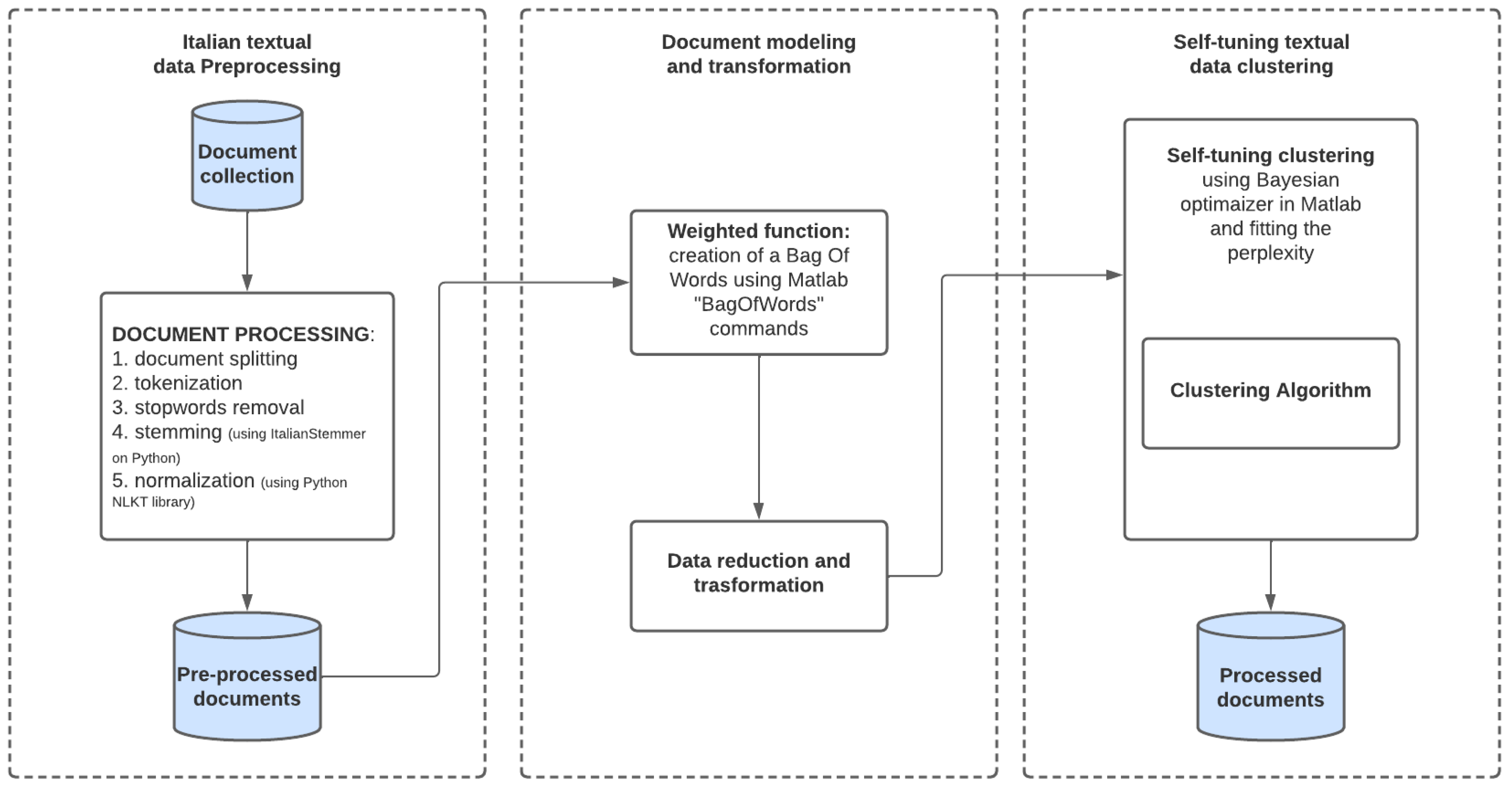
While the previous sections describe some theoretical foundations of the TM algorithm considered in our study, this section presents the pre-processing phase implemented on the data set. It includes an initial data acquisition step of text transcriptions, text cleaning, and a word simplification step. These last two steps employ algorithms, such as tokenization, normalization, removal of stopwords, and stemming. Finally, a data transformation is implemented, in which each word is associated with a numerical value, thus forming the input matrix of the TM algorithm.

The focus of this study is on the Italian natural language. Since in Matlab, the language support of the environment is limited to English, Japanese, Korean, and German only, in our research, we implemented the steps of the pre-processing phase in Python environment by defining an Italian resource database for text analysis. As we aim to support the development of NLP algorithms for the Italian natural language, the complete list of Italian stopwords implemented in our research is available on request as additional material for this paper.

The details about data pre-processing are as follows:

• Tokenization and case normalization. The text of transcriptions is split into words named tokens. Letters in each token are all transformed into lower case characters (lowercasing). After tokenization, punctuation, special characters, and short words (with less than three characters) are removed. SpaCy is the NLP library in Python used for the elaboration of text, in the Italian natural language, in our study.
• Stopwords removal. The meaningless words (such as articles or prepositions) are also removed since they do not add any information to the analysis. Stopwords are the terms that have scarce meaning and occur in the document with high frequencies, such as delimiters and prepositions. It is important to note that the number of stopwords in the Italian natural language is greater than those in other languages, such as English.
• Stemming. Words are stripped of prefixes and suffixes, reducing them to their most basic form (stem). This step minimizes the size of the dictionary and groups terms that have the same root. It is worth noticing that for the Italian language vocabulary, which presents several prefixes or suffixes for the same root, stemming could result in a more complex task in comparison to other languages, such as English [16].

After pre-processing, the text is represented in the bag-of-words form, which describes texts, disregarding the terms order and the grammar rules but representing the main themes.

To identify the proper topic of a document, weights must be assigned to words to measure the relevance the terms have in the transcriptions. These weights are computed as the product of local and global measures. The local measures refer to the significance that a word has within the document. The global measures concern the whole data set of transcriptions. Weights are stored in a matrix, in which rows are associated with the documents and columns with the words. In our study, we combined weights from both the categories: term frequency (tf) for the local weights, and inverse document frequency (idf) for global weights.

This phase is followed by the fitting of the model and by the identification of the top words for each topic. A general schema of the algorithm implemented in our study is summarized in Figure 1.

5. Case Study

The case study of this paper is a collection of transcriptions of telephone conversations between an agent (telephone operators) of the assistance service of an energy supplier and real-world customers. The data set of $M=993$ transcriptions was validated, anonymized, and shared by an Italian customer support center via a .json file.

To date, the customer support center manually carries out the operation of reading every single telephone transcription. The objective is to identify the most relevant topics that emerge during the telephone call. As stated in the introduction section, the semantic restructuring of a significant amount of data provides more efficient information management.

In this case study, the company needs to consult the database of telephone recordings very quickly, searching for a specific telephone transcription using keywords. It is not uncommon for an operator engaged in a phone call to have to consult previous similar cases to propose solutions in real time to the user connected to the telephone, hence the importance of implementing automatic information management.

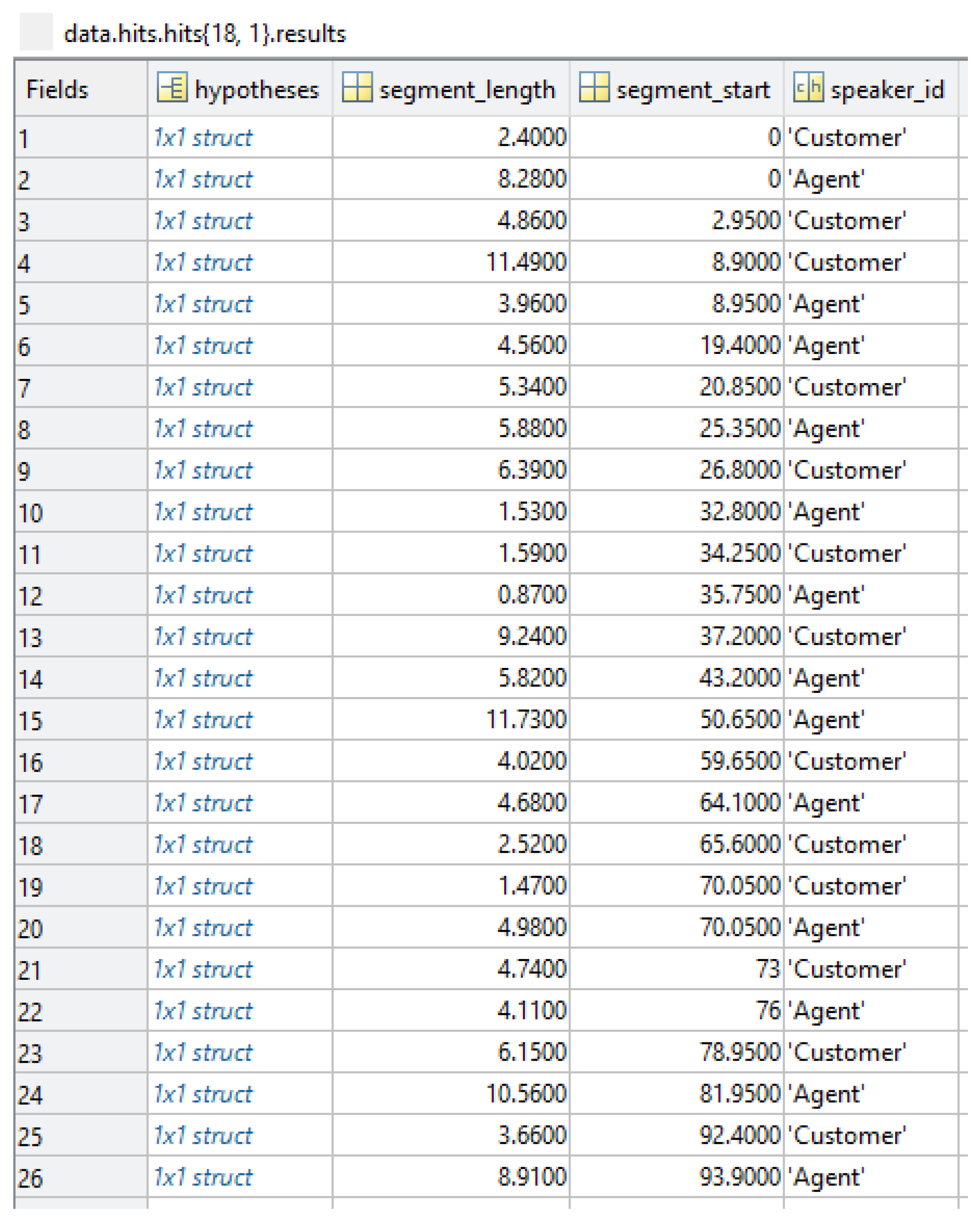
The data set (corpus) is organized at three levels of detail:

• In the first level of detail, each transcription is separated into segments, reporting the speech of the operator (‘Agent’) to that of the customer (‘Customer’). For each part, the duration of the speech in seconds is also recorded. An example of data at the first level of detail in the Matlab environment is in Figure 2.
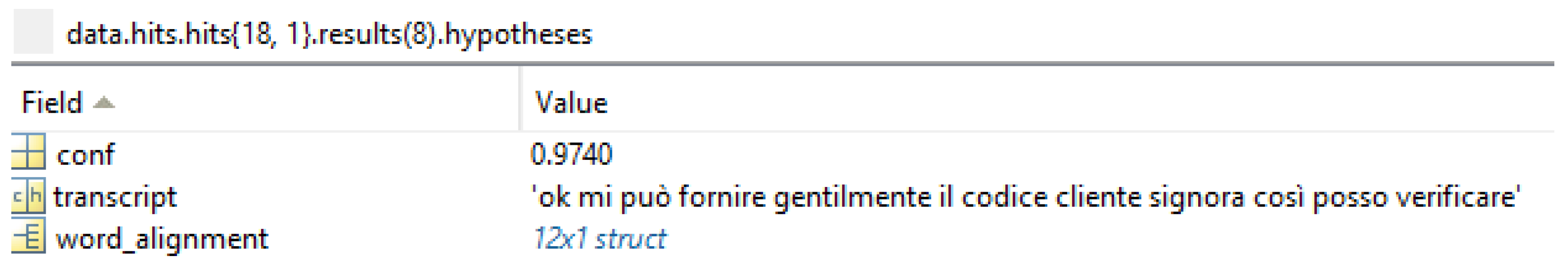
• In the second level of detail, there is the textual transcription in string format of the single segment. The text message’s confidence value is recorded at this level. An example of data at the second level of detail in the Matlab environment is in Figure 3.
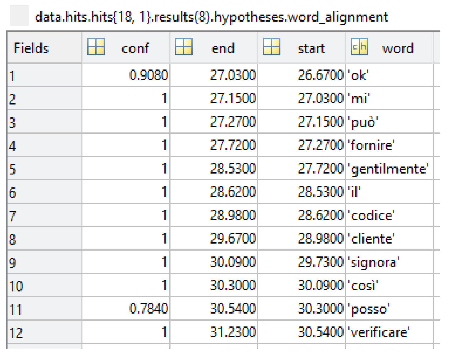
• In the third level of detail, each transcription is separated into words. Each word is associated with a confidence value and the time location within the transcription. An example of data at the third level of detail in the Matlab environment is in Figure 4.

5.1. Algorithm Implementation

The TM algorithm was implemented in Matlab R2021b. The Text Analytics Toolbox was used for the LDA algorithm both for modeling and prediction and the presentation of results through appropriate graphs (word-cloud graphs). It is worth noticing the availability of particular application programs interfaces (APIs) that allow integration between the Matlab and Python environments.

The first step is to extract and save the textual information contained in the .json file in a specific Matlab variable. We decided to keep track during this phase, in addition to the text of the phone call, of the ‘speaker id’ label. Short or empty transcriptions were removed, as they are useless in the TM algorithm. The pre-processing steps are as in the following pre-processing algorithm (Algorithm 1).

Algorithm 1: Pre-processing.

for m=1:M do    1. tokenizedDocument($d_m$)    2. lower($d_m$)    3. erasePunctuation($d_m$)    4. stemming($d_m$)    5. removeWords($d_m$) / removeStopWords($d_m$)    6. bagOfWords(D)    7. tfidf(BoW) end for

Step 4, stemming, is the most important, as it significantly reduces the dimensional complexity of a text analysis problem. An example of stemming in the Italian natural language is as follows. The words “disdire”, “disdetto”, “disdetta” (the Italian for “service cancel”) in the stemming step produce the following result:

Stemming

“disdire” -> “disd”

“disdetto”, “disdetta” -> “disdett”

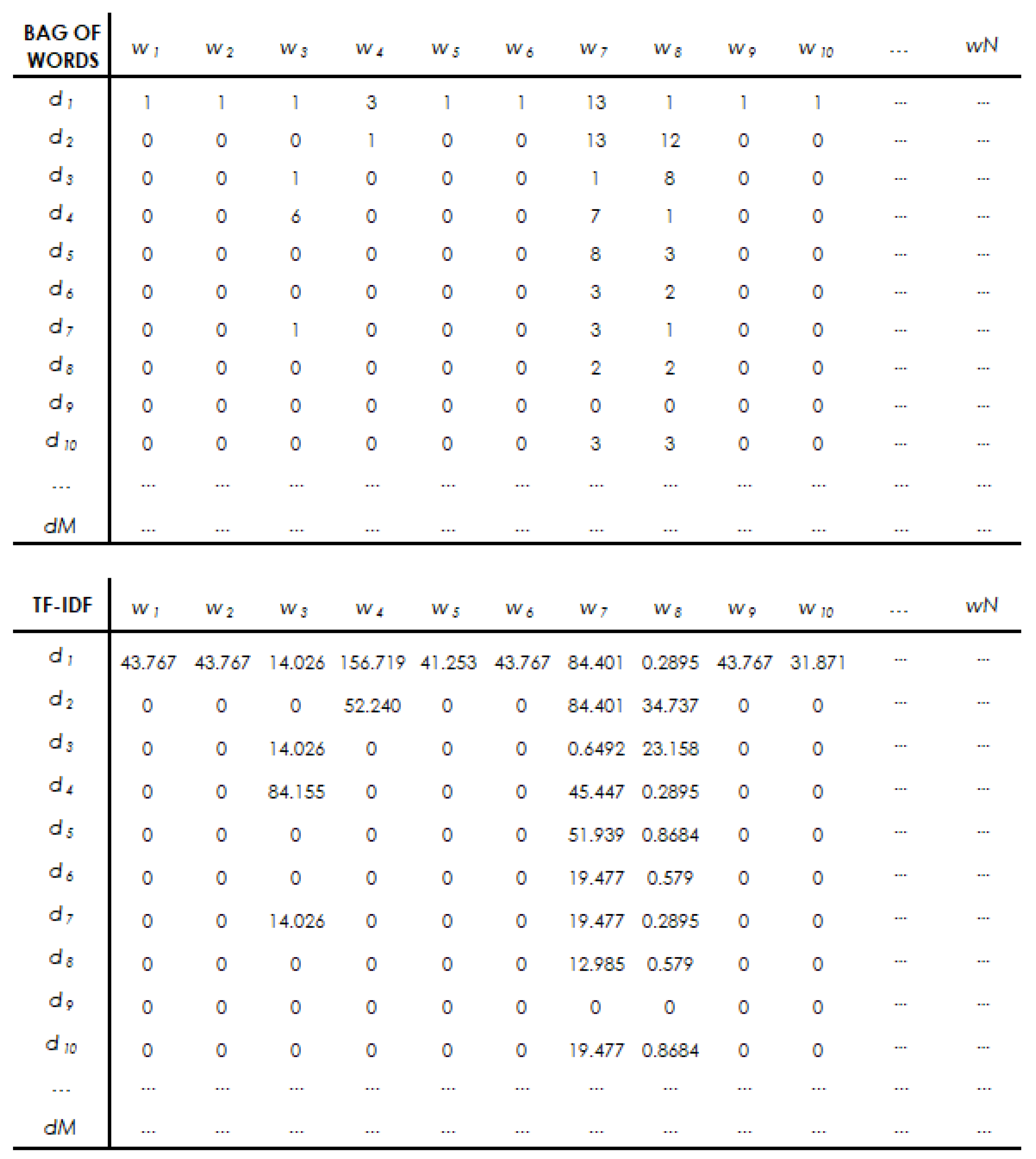
With reference to step tfidf in Algorithm Pre-processing, following Figure 5 shows the result on a portion of the matrix (10 documents and 10 words). Consider the words $w_3$ and $w_7$ for the document $d_4$. The second word has a higher number of occurrences than the first (7 versus 6 in the bag-of-words table); following the TF-IDF correction, the weight associated with the most recurring word is about half that of the least recurring word. This happens because, limited to the small portion of the corpus represented, the word $w_7$ is also used several times in the other 9 documents, while the word $w_3$ is missing in many of them.

The working environment chosen is VS code, with a base kernel Python 3.10.2. The NLTK—Natural Language Toolkit library was used The library contains all the built-in functions necessary to perform the preprocessing. In particular, the normalization of words is carried out through a Python stemmer built for the Italian natural language. The .py script takes as input the three .csv files exported by Matlab (data, agent and customer). The LDA algorithm, coded in Matlab R2021b ran on a 2.6 GHz Intel Core i7 with 16 GB of memory.

5.2. Model Optimization

In our study, the following settings for the LDA models were used. The maximum number of iterations that the model has to converge was set to be equal to $T=250$, the implemented optimizer (or inference algorithm used to estimate the LDA model) was selected in a set of four listed below.

• cgs—collapsed Gibbs sampling. It can be more accurate at the cost of taking longer to run [26].
• avb—approximate variational Bayes. It typically runs more quickly than collapsed Gibbs sampling and collapsed variational Bayes, but can be less accurate [41].
• cvb0—collapsed variational Bayes. It can be more accurate than approximate variational Bayes at the cost of taking longer to run [42].
• savb—stochastic approximate variational Bayes. It is best suited for large datasets [43].

The possible range of topic value K was set between a minimum of 5 and a maximum of 40. In our case study, a number equal to 5 was considered the lowest possible number of clusters to divide the corpus in, and 40 was considered an acceptable upper bound, since having more clusters leads to results that are complex to be analyzed and validated. The LDA parameters, $\alpha$ value, and the $\beta$ value should be greater than or equal to 0. The value set for this parameter was $\alpha =50/K$ and the value set for $\beta$ was $\beta =0.1$, according to the literature [44].

The performance metric selected in our study is the “perplexity” value. It inversely measures the statistical likelihood that data, in the case study, are generated by the LDA model. Hence, a lower “perplexity” indicates a higher likelihood value and better model performance. “Perplexity” was computed using the inverse of the geometric mean of token likelihood within the test corpus. Low “perplexity” values, in other words, suggest strong consistency between word distributions in test documents and outputs from training topics.

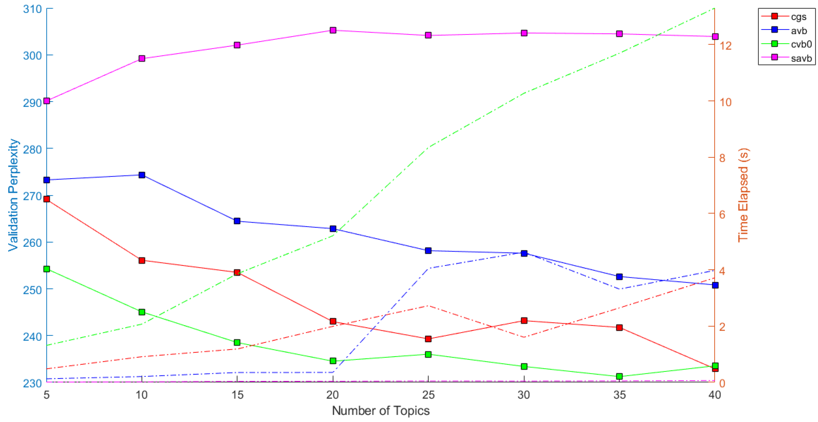
Figure 6 depicts the “perplexity” trend for the four inference algorithms used to estimate the LDA model and for topics number K ranging between 5 and 40. From Figure 6, it appears that for the cgs, avb and cvb0 optimizer, the “perplexity” curves decrease nearly monotonically with the increase in the number of topics, which demonstrates that LDA can refine the statistical model as more topics are considered. On the other hand, for savb optimizer, the “perplexity” does not show a clear decreasing trend with the growth in the number of topics.

In terms of computational performance, it results that the collapsed variational Bayes approach cvb0, despite presenting the best performance in terms of “perplexity” for any number of topics K ranging between 5 and 40, and also requires the most significant computational time to run, when compared to all the other methods. The plot in Figure 6 also suggests that fitting a model with topics ranging between 20 and 25 may be a good choice. Increasing the number of topics may lead to a better fit, but fitting the model takes longer to converge. Since we also observed from our experimental results the redundancy of topics meaning for large values of K, we decided to set $K=20$ as the proper choice of topic number for the reference case study.

From the results graphically reported in Figure 6, and by considering the trade-off between performance measures in terms of “perplexity” and computational time, it appears that the CGS-based LDA classification model performs better than the VB-based models. Therefore, the  CGS-based LDA classification model results in the most satisfactory approach in our case study.

5.3. Topic Modeling Results

The 20 resulting topics, identified by the three most representative words, are shown in the following

Table 1. Top 3 words for the 20 topics.

Topic $k=1$: bollett, scadenz, qualit	Topic $k=11$: catastal, rilasc, spost
Topic $k=2$: luc, gas, scadenz	Topic $k=12$: distributor, ritorn, amministr
Topic $k=3$: autolettur, gas, rilev	Topic $k=13$: conguagl, gest, misur
Topic $k=4$: gas, luc, quot	Topic $k=14$: banc, addeb, bollett
Topic $k=5$: gas, disponibil, rientr	Topic $k=15$: caldai, pap, privacy
Topic $k=6$: energ, verr, bimestral	Topic $k=16$: proprietar, met, test
Topic $k=7$: fornitor, blocc, confront	Topic $k=17$: moros, sald, altern
Topic $k=8$: energ, dimentic, ital	Topic $k=18$: gas, disdett, cessazion
Topic $k=9$: gas, luc, car	Topic $k=19$: bollettin, bonif, fax
Topic $k=10$: qualit, societ, quadr	Topic $k=20$: voltur, ident, gas

.

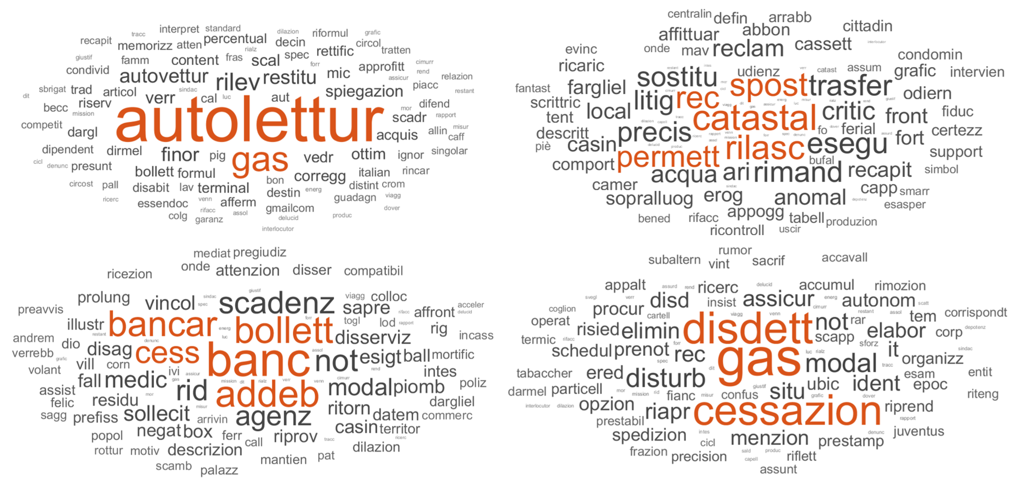
To visualize the topic content, we used the word-cloud technique. The word-cloud graph represents the terms that most probably describe the topics according to the LDA model. The clouds represent the topic–term matrices. Comparison of the cloud sets obtained by different models is left to the analyst’s judgment. A word-cloud visualization emphasizes the terms with the highest probabilities with bigger font sizes. It is possible to observe if the classification results are satisfactory or if the TM approach has not produced acceptable results. Because of its clearness and simplicity, the word-cloud representation is widely used in the literature to visualize the results of the LDA topic modeling [45].

Figure 7 shows some word-cloud graphs by way of example. For example, the word-cloud of topic 3 identifies the problem of self-reading of the gas meter and a probable error in quantifying consumption. Topic 11, on the other hand, implies the need to find cadastral information to probably carry out a new domiciliation. Continuing with the other examples, we can see that topic 14 highlights the customer’s willingness to debit the bill on their bank account, while topic 18 highlights the issue of termination or cancellation of the contract.

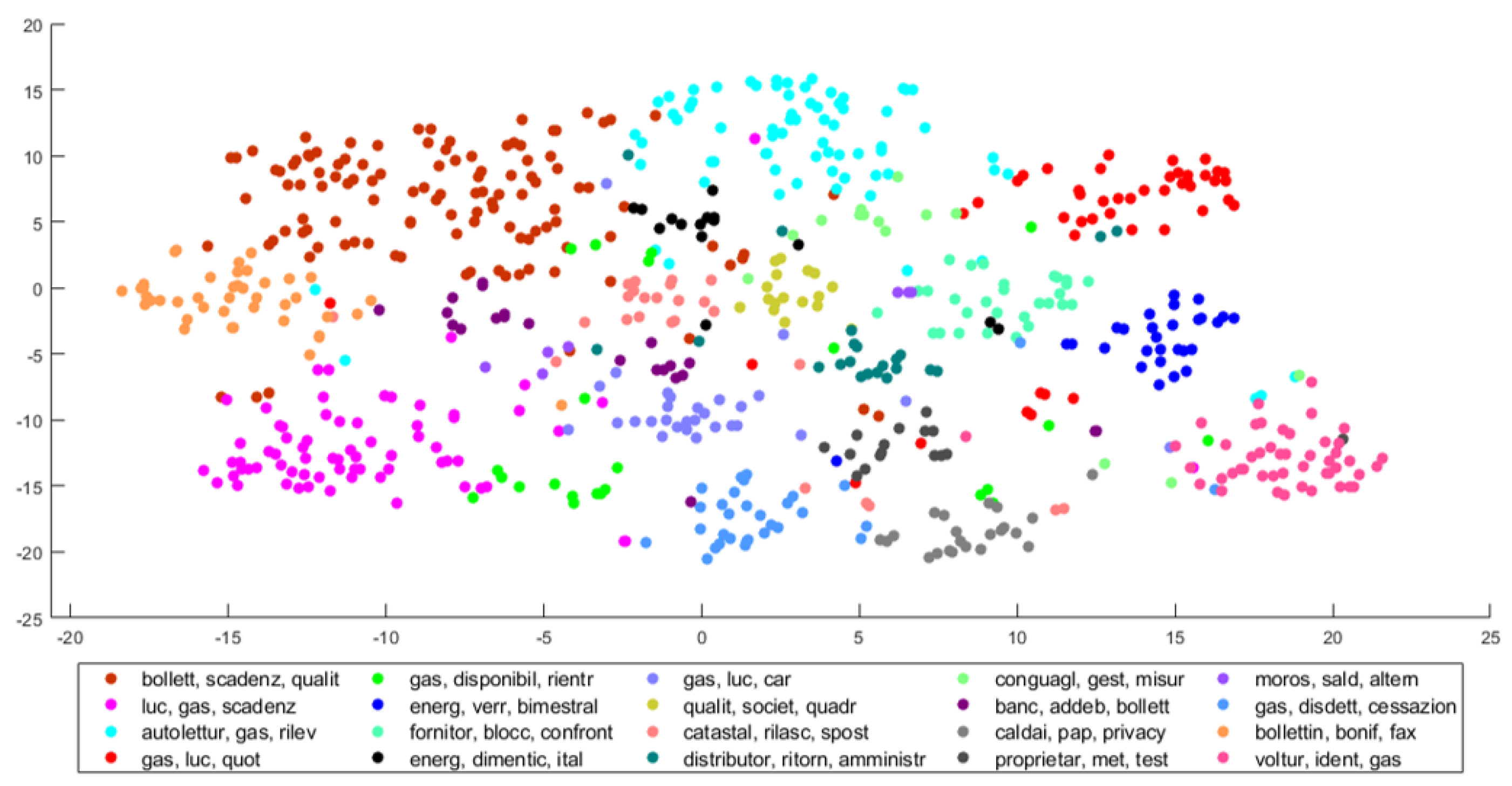
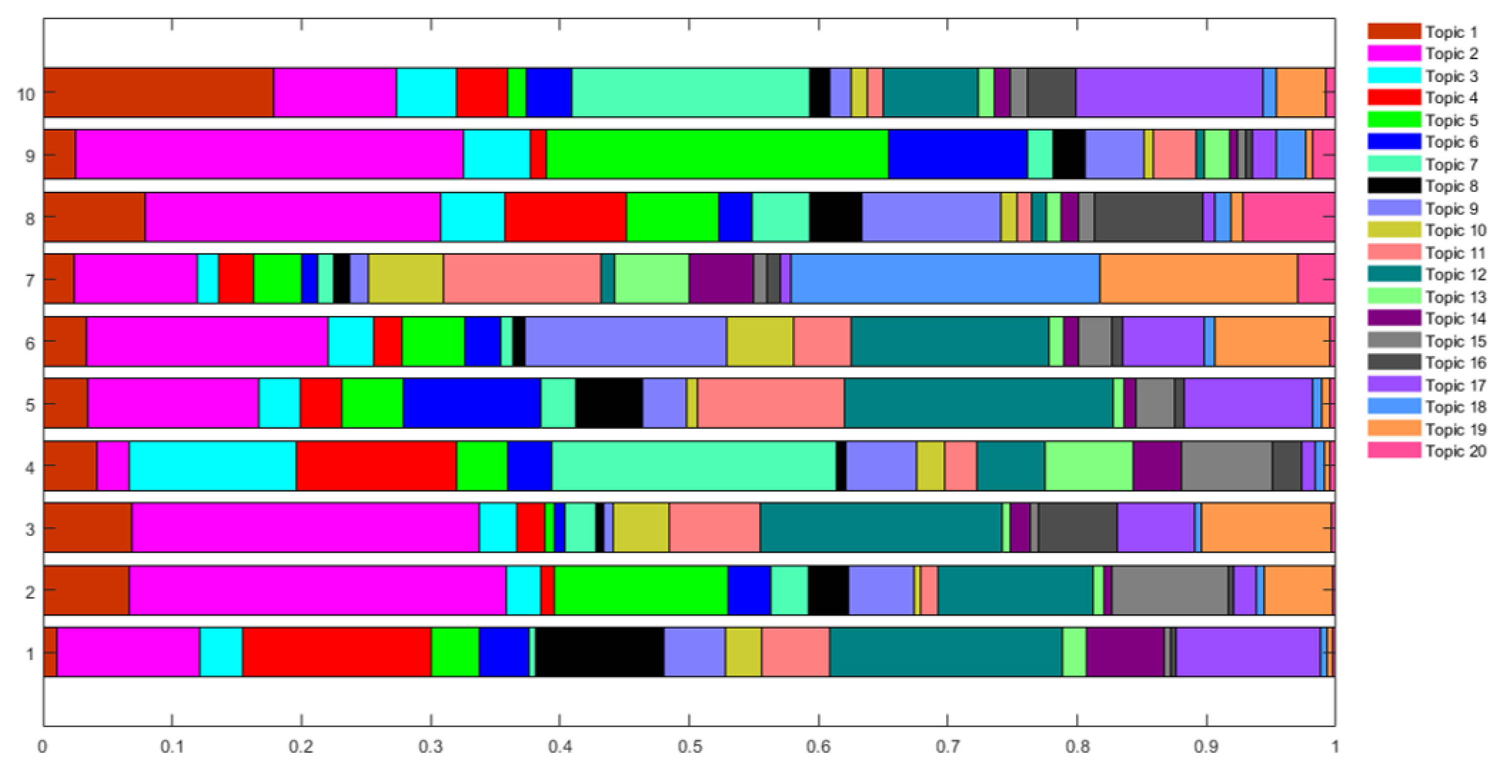
For multidimensional vectors, the t-distributed stochastic neighbor embedding (t-SNE) is a 2D projection method [46]. This embedding allows viewing similarities between multidimensional vectors and plot clusters of similar documents. The results of the case study are depicted in Figure 8. The main output is the distribution of topic probabilities for each document ${\theta }_{m,k}$. For the first 10 documents, we represent the values ${\theta }_{m,k}$ for $m=1\dots 10$ and $k=1\dots 20$ and in graphic form in the following Figure 9.

6. Conclusions

In past research, the use of TM methods for the Italian natural language was rarely considered. In the present study, we introduced a case study in the Italian natural language. The proposed methodology was implemented by the integration of Matlab and Python, using the library “ItalianStemmer” and command bag of words. In this regard, it is essential to use the Matlab API to perform Python functions within the environment.

A comparison of four inference algorithm used to estimate the LDA model demonstrated that, considering the trade-off between performance measure in terms of “perplexity” and computational time, the CGS-based LDA classification model performs better than the VB-based models. Hence, the CGS-based LDA classification model results in the most satisfactory approach in our case study.

From the obtained experimental results of the CGS-based LDA, we can assess that TM performs adequately in describing the transcriptions under analysis, and can cluster the documents based on their content. The developed approach is based on an Italian dictionary, and hence, on a bag of words with Italian terms. The results obtained from the datasets considered in the use case confirm the clusters to be well separated. The topic turns out to be helpful for analysts in the analytic tasks. The analyst can choose to assign to the document words several relevances by using different weights. Similarly, the analyst can choose the granularity level required for the analysis (through the different K values) and several evaluation tools that highlight different features of the clustering, to evaluate the findings. Our case study shows that the TM can effectively lead the analysis process of textual data collections.

Possible extensions of the current study are as follows: (i) the investigation of different probabilistic data transformation methods; (ii) the design of a self-learning strategy that can suggest adequate configurations; and (iii) the refinement of the topic semantic description to achieve better modeling for a given data set in the specific case study of our study.