Abstract
Predictive Process Monitoring (PPM) has been integrated into process mining use cases as a value-adding task. PPM provides useful predictions on the future of the running business processes with respect to different perspectives, such as the upcoming activities to be executed next, the final execution outcome, and performance indicators. In the context of PPM, Machine Learning (ML) techniques are widely employed. In order to gain trust of stakeholders regarding the reliability of PPM predictions, eXplainable Artificial Intelligence (XAI) methods have been increasingly used to compensate for the lack of transparency of most of predictive models. Multiple XAI methods exist providing explanations for almost all types of ML models. However, for the same data, as well as, under the same preprocessing settings or same ML models, generated explanations often vary significantly. Corresponding variations might jeopardize the consistency and robustness of the explanations and, subsequently, the utility of the corresponding model and pipeline settings. This paper introduces a framework that enables the analysis of the impact PPM-related settings and ML-model-related choices may have on the characteristics and expressiveness of the generated explanations. Our framework provides a means to examine explanations generated either for the whole reasoning process of an ML model, or for the predictions made on the future of a certain business process instance. Using well-defined experiments with different settings, we uncover how choices made through a PPM workflow affect and can be reflected through explanations. This framework further provides the means to compare how different characteristics of explainability methods can shape the resulting explanations and reflect on the underlying model reasoning process.
1. Introduction
1.1. Problem Statement
Predictive process monitoring (PPM) is a use case of process mining [1], which supports stakeholders by providing predictions about the future of a running business process instance [2,3]. A process instance represents one specific execution instance out of all possible ones enabled by a business process model. Both process mining and PPM aim at informing stakeholders on how a business process is currently operating or expected to operate in near future. However, using ML models as prediction black-boxes does not help achieve this purpose. As stakeholders engagement is at the center of process mining tasks, performance as well as accuracy are no longer sufficient as metrics for evaluating a PPM prediction task. Stakeholders also need to assess the validity of the reasoning mechanisms being at the heart of the predictive model, as the model is predicting the future state of running business process instances. Justifying predictions to their recipients, in turn, increases the users’ trust, engagement and advocacy of PPM mechanisms.
The need to justify predictions prompted the introduction of eXplainable Artificial Intelligence (XAI) [4], with methods and mechanisms proposed to provide explanations of predictions generated by an ML model [5,6,7,8,9,10,11,12]. These explanations are expected to reflect how a predictive model is influenced by different choices made through a given PPM workflow. Moreover, PPM tasks employ specific mechanisms that allow aligning process mining artefacts to ML models requirements. Different XAI methods exist to address explainability needs in the context of PPM, but the assumption remains that these methods should provide simple and consistent explanations for a given prediction scenario. However, explanations may vary due to changes in scenario settings or due to their underlying generation mechanisms. Studying how explanations of XAI methods may vary is therefore a crucial step to understand the settings suitable for employing these methods, as well as the way to interpret explanations in terms of the underlying influencing factors.
With the increasing number of XAI methods which address different purposes and users needs through varying techniques, there is a need to compare different XAI methods outcomes given the same PPM workflow settings. Note that such a comparison is beneficial to identify combinations of techniques that if adopted through a PPM project can maximize the gains of applying XAI methods. Contrasting and differentiating XAI methods enables us to discover situations for which certain methods are better able to highlight data or ML models characteristics through generated explanations than others. Such differentiation is crucial to facilitate the selection of XAI methods, which not only suit the input characteristics, but are, in addition, well-fitting to the purpose of explaining PPM outcomes and to the target audience. Providing a guidance on XAI methods available choices based on experimental studies is a step towards integrating explainability as an indispensable stage of any project involving generation of predictions.
1.2. Contributions
With an attempt to address the need to understand and gain insights into the application of XAI methods in the context of PPM, this paper provides:
- A framework for comparing the explanations produced by XAI methods globally and locally (i.e., for the entire event log or for selected process instances), separated and against each other. The comparison framework uses different PPM workflow settings with predefined criteria based on the underlying data, predictive models and XAI methods characteristics.
- An empirical analysis of explanations generated by three global XAI methods, as well as two local XAI methods for predictions of two predictive models over process instances from 27 event logs preprocessed with two different preprocessing combinations.
Section 2 provides background information on basic topics needed for understanding this work. In Section 3, we highlight the basic research questions investigated in this paper. In Section 4 and Section 5, we discuss the experimental settings, experiment results, and experiment observations. Section 6 highlights the lessons learned and provides conclusions that allow answering the basic research questions. Related work is discussed in Section 7. Finally, we conclude the paper in Section 8.
2. Preliminaries
This section introduces basic concepts and background knowledge necessary to understand our work. Section 2.1 introduces PPM and associated steps to carry on predictions of information relevant to a running business process. Then, we discuss available explainability methods with an in-depth look into those methods that address tabular data which constitutes the focus of this work.
2.1. Predictive Process Monitoring
Predictive Process Monitoring (PPM) addresses a critical process mining use case providing predictions about the future state of a running business process execution instance via building predictive models. Examples of PPM tasks include the next activity to be carried out, time-related information (e.g., elapsed time, remaining time till the end), outcome of the process instance, execution cost, or executing resource [1]. Event logs constitute the input to PPM tasks. More precisely, they document the execution history of a process as traces, each of which representing execution data belonging to a single business process instance. A trace contains mandatory attributes, such as case identifier, event class, and timestamp [1]. A trace may contain dynamic attributes representing information about a single event. Resources fulfilling tasks and documents associated with each event constitute examples of dynamic attributes. Besides dynamic attributes there are static attributes, which have constant values for all events of a given trace.
PPM Workflow
According to the previously reported survey results [2,3], a PPM task follows two stages, offline and online. Each stage has steps, and the two stages together with their corresponding steps constitute a PPM workflow.
- 1
- PPM Offline Stage. This stage starts with constructing a prefix log from the input event log. A prefix log is needed to provide a predictive model with incomplete process instances (i.e., a partial trace) for the training phase of an ML model. Therefore, prefixes can be generated by truncating process instances in an event log up to a predefined number of events. Truncating a process instance can be done up to the first k events of its trace, or up to k events with a gap step (g) separating each two events, where k and g are user-defined. The latter prefixing approach denoted as gap-based prefixing.Prefix preprocessing sub-steps include bucketing and encoding. Prefix bucketing groups the prefixes according to certain criteria (e.g., number of activities or reaching a certain state during process execution). The former criteria are defined by the bucketing technique [3]. Single, state-based, prefix length-based, clustering, and domain knowledge-based are examples of prefix bucketing techniques. Encoding is the second sub-step of prefix preprocessing. Prefix encoding involves transforming a prefix to a numerical feature vector that serves as input to the predictive model, either for training or making predictions. Encoding techniques include static, aggregation, index-based, and last state techniques [2,3].In the following step, a predictive model is constructed. Depending on the PPM task, an appropriate predictive model is chosen. The prediction task type may be classification or regression. Next, the predictive model is trained on encoded prefixes representing completed process instances. For each bucket, a dedicated predictive model needs to be trained, i.e., the number of predictive models depend on the chosen bucketing technique. Finally, the performance of the predictive model needs to be evaluated.
- 2
- PPM Online Stage. This stage starts with a running process instance that has not completed yet. Buckets formed in the offline stage are recalled to determine the suitable bucket for the running process instance, based on the similarity between the running process instance and the prefixes in a bucket. The running process instance is then encoded according to the encoding method chosen for the PPM task. The encoded form of the running process instance constitutes the input for the prediction method after having determined the relevant predictive model from the models created in the offline stage. Finally, the predictive model generates a prediction for the running process instance according to the predefined goal of the PPM task.
2.2. eXplainable Artificial Intelligence
PPM inherits the challenges faced by ML approaches, as a reasonable consequence of employing the latter approaches. One of these challenges concerns the need to gain user trust in the generated predictions, which promotes growing interest in the field of explainable artificial intelligence (XAI). An explanation is “a human-interpretable description of the process by which a decision maker took a particular set of inputs and reached a particular conclusion” [13]. In the context of our research, the decision maker is an ML-based predictive model. Transparency is considered a crucial aspect of explainability. Model transparency can be an inherent characteristic or be achieved through an explanation. Transparent models are understandable on their own and satisfy one or all model transparency levels [14]. Linear models, decision trees, Bayesian models, rule-based learning, and General Additive Models (GAM) [4] may all be considered as transparent (i.e., interpretable) models. Note that the degree of transparency realised through an explanation may be affected by several factors, e.g., the incompleteness of the problem formulation or understanding, the level of complexity of an explainability solution, and the number as well as length of cognitive chunks made available to the user through an explanation.
Several approaches are proposed under the umbrella of explainability. Explanations construction approaches can be categorised along several dimensions (cf. Figure 1). We use dashed rectangles to highlight those techniques that we further consider for studying in our comparative framework. In the following, we illustrate these explainability dimensions.
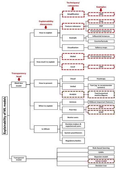
Figure 1.
Explainability taxonomy in ML.
- 1
- How to explain. This dimension is concerned with the approach used to explain how a predictive model derives its predictions based on the given inputs. Corresponding approaches have been categorised along different perspectives including design goals and evaluation measures, transparency of the explained model and explanation scope [14,15], granularity [16], and relation to the black-box model [17]. For example, a group of approaches tend to generate an explanation by simplification. These approaches simplify a complex model by using a more interpretable model called a surrogate or proxy model. The simplified model is supposed to generate understandable predictions that achieve an accuracy level comparable to the black-box one. Another group of approaches study feature relevance. They aim to trace back the importance of a feature for deriving a prediction. Another family of approaches tend to explain by example. Approaches from this category tend to select representative samples that allow for insights into the model’s internal reasoning [14,16]. The final category in this dimension explains through visualisation, i.e., intermediate representations and layers of a predictive model are visualised with the aim to qualitatively determine what a model has learned [16].Approaches belonging to this XAI dimension are further categorised into model-agnostic or model-specific methods. Model-agnostic approaches are able to explain any type of ML predictive models, whereas model-specific approaches can only be used on top of specific models.
- 2
- How much to explain. An explanation may be generated at various levels of granularity. An explanation effort can be localised to a specific instance, i.e., local explanation, and it can provide global insights into which factors contributed to the decision of a predictive model, i.e., to generate global explanations. The scope of an explanation and, subsequently, the chosen technique depend on several factors. One of these factors is the purpose of the explanation, e.g., whether it shall allow debugging the model or gaining trust into its predictions. Target stakeholders constitute another deterministic factor. For example, an ML engineer prefers gaining a holistic overview of the factors driving the reasoning process of a predictive model, whereas an end user is only interested in why a model made a certain prediction for a given instance.
- 3
- How to present. Choosing the form according to which an explanation is presented is determined by the way the explanation is generated, the characteristics of the end user (e.g., level of expertise), the scope of the explanation, and the purpose of generating an explanation (e.g., to visualise effects of feature interactions on decisions of the respective predictive model). Three categories of presentation forms were introduced in [15]. The first category comprises visual explanations that use visual elements like saliency maps [10] and charts to describe deterministic factors of a decision in accordance with the respective perspective to be explained of a model. Verbal explanation provides another way of presenting explanations where natural language is used to describe model reasoning (e.g., in recommender systems). The final form of presentation is analytic explanation where a combination of numerical metrics and visualisations are used to reveal model structure or parameters, e.g., using heatmaps and hierarchical decision trees.
- 4
- When to explain. This dimension of an explainability approach is concerned with the point in time an explanation shall be provided. Agreeing on explainability being a subjective topic and depending on the receiver’s understanding and needs, we may regard explainability provisioning from two perspectives. The first perspective considers explainability as gaining an understanding of decisions of a predictive model, being bounded by model characteristics. Adopting this perspective imposes explainability through mechanisms put in place while constructing the model to obtain a white-box predictive model, i.e., intrinsic explanation. On the other hand, using an explanation method to understand the reasoning process of a model in terms of its outcomes is called post-hoc explanation. The latter provides an understanding in terms of the whole reasons behind the mapping process between inputs and outputs. Moreover, it provides a holistic view of input characteristics which led to predictive model decisions.
- 5
- Explain to Whom. Studying the target group of each explainability solution becomes necessary to tailor the explanations and to present them in a way that maximizes the interpretability of a predictive model, forming a mental model of it. The receivers of an explanation should be at the center of attention when designing an explainability solution. These receivers can be further categorised into different user groups including novice users, decision makers and experienced users, system practitioners, and regulatory bodies [14,15]. Targeting each user group with suitable explanations contributes to achieve the explanation process purpose. The purpose of an explanation may be to understand how a predictive model works or how it makes decisions, or which patterns are formed in the learning process. Therefore, it is crucial to understand each user group, identify its relevant needs, and define design goals accordingly.
The various dimensions of explainability are tightly interrelated, i.e., a particular choice in one dimension might affect the choices made in other dimensions. Making choices on the different dimensions of the presented taxonomy is guided by several factors, which include the following: (1) enhancing understandability and simplicity of the explainability solution; (2) the availability of software implementations of explainability methods and whether these implementations are model-agnostic or specific; (3) the type of output of each explanation method and the subsequent choice of a suitable presentation type which suits the target group. When facing explanations that serve different user groups with different explainability goals, putting explainability evaluation techniques in place becomes a necessity.
3. Research Questions
The goal of this research is to study how explanations are affected by underlying PPM workflow-related choices. It is crucial to study the different characteristics of XAI methods that influence the final outcome of explanation process. Overall, this leads to the following research questions (RQ)s:
RQ: How can different XAI methods be compared? Conducting a benchmark study that allows comparing all available explainability approaches is not likely to be possible [18]. This is due to the varying characteristics of these approaches in terms of the dimensions (cf. Section 2.2). However, as many techniques have been proposed for evaluating explanations [18,19], a constrained study would be useful to compare the relative performance of explainability methods that have been applied in the context of PPM approaches. In addition, the consistency of explainability methods applied to PPM results needs to be studied in order to shed light on one of the potential vulnerabilities of XAI methods, namely sensitivity of explanations, i.e., how several conditions can affect the ability of XAI methods to generate the same explanations again under the same settings. An example of the conditions affecting the reproduction of explanations is the inability to regenerate the same neighborhood of the process instance to be explained in presence of high-dimensionality data. To this end, we subdivide RQ into the following sub-research questions:
RQ1: To what extent are explanations consistent when executing an explanation method several times using the same underlying settings?.
RQ2: How are the explanations generated by an XAI method affected by predictive model choices?
Explainability methods vary by the extent to which an explanation can be generalised over several data samples that belong to the same vicinity (i.e., the same neighborhood which defines underlying similarities unifying data samples belonging to it). Explainability methods also vary in the granularity of the explanations they provide and their suitability to explain a number of data samples independent of whether they are small or large, i.e., independent of whether the explainability method is local or global. However, the number of explained data samples comes with computational costs. Therefore, we add another sub-research question to compare explainability methods with respect to their execution time:
RQ3: How do explainability methods differ in terms of execution time? How does needed time differ with respect to different dataset characteristics, preprocessing choices, and chosen predictive models?
4. XAI Comparison Framework
This section describes dimensions of the framework we propose and use to compare basic XAI methods. For the basic infrastructure of a PPM outcome prediction task, we are inspired by the work of Teinemaa et al. [3,20]. We preserve the settings used in [3] to observe their impact given the reported performance of studied predictive models and preprocessing techniques from an explainability perspective.
Figure 2 shows the components of our framework organized under dimensions resembling an ML model creation pipeline aligned with the PPM offline workflow, and incorporating an explainability-related dimension. These dimensions provide means to categorise our experiments with the aim of answering the research questions introduced in Section 3. These dimensions are further discussed in this section. We apply all available combinations in each dimension, in a dedicated experiment, while fixing other options from other dimensions.
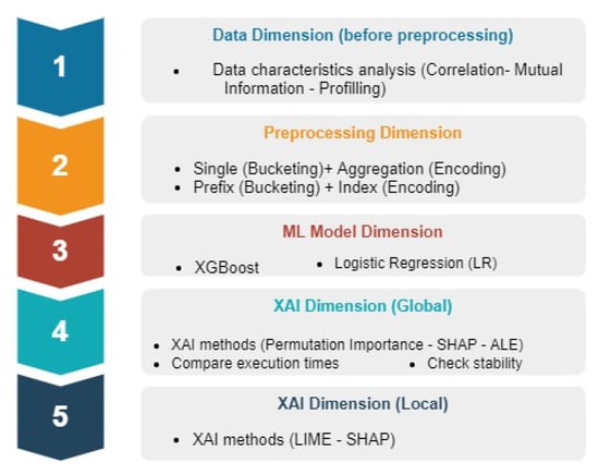
Figure 2.
XAI Comparison Framework Components.
4.1. Framework Composition
In this subsection, we describe the building blocks of our comparison framework, including data, chosen preprocessing techniques, selected predictive models, and XAI algorithms. Categorising our setups and the techniques we use (cf. Figure 2) is accomplished with the aim of studying the impact of modifying different parameters at each dimension on the resulting explanations.
4.1.1. Data Dimension
This dimension involves studying the complete characteristics of the data to be used in the experiments whose outcomes shall highlight potential implications on the reasoning process of an ML model. The complete set of experiments in this dimension include constructing data profiles of the used event logs, studying Mutual Information (MI) between input features and the target, and studying correlations between the features. The complete outcomes of the analyses are made available in a complementary study we conducted [21]. The data perspective in our experiments on the proposed framework build on using three real-life event logs that are publicly available from the 4TU Centre for Research Data [22]. The chosen event logs vary in the considered domain (healthcare, government and banking), the number of traces (representing process instances), and the number of events per trace. The event logs further vary in the number of static and dynamic attributes, the number of categorical attributes and, as a result, the number of categorical levels available through each categorical attribute. The three basic event logs we used are as follows:
- Sepsis. This event log belongs to the healthcare domain and reports cases of Sepsis as a life threatening condition.
- Traffic fines. This event log is governmental and is extracted from an Italian information system for managing road traffic fines.
- BPIC2017. This event log documents load application process in a Dutch financial institution.
Several labelling functions allow classifying each process instance into one of two classes, i.e., a binary classification task [3]. Applying different labelling functions results in sub-versions for some of the event logs. These labelling variations result in three extracted logs from the Sepsis event log (Sepsis 1, 2, 3), and three logs extracted from the BPIC2017 event log (BPIC2017_(Refused, Accepted, Cancelled)). These different labelling functions increased the number of used event logs from three to seven event logs. Table 1 shows basic statistics of the event logs used in our experiments. These event logs are cleaned, transformed, and labelled according to the rules defined by the framework available in [3].

Table 1.
Event logs statistics.
4.1.2. Preprocessing Dimension
We make two choices about bucketing and encoding preprocessing techniques. To bucket the traces of chosen event logs, we apply single bucketing and prefix-length bucketing, with a gap of 5 events. Moreover, we apply aggregation and index-based encoding techniques. Usually both encoding techniques are coupled with static encoding to transform static attributes into a form in which they can serve as input to a predictive model. As a result, we obtain two combinations of bucketing and encoding techniques i.e., single-aggregation and prefix-index. As index encoding leads to dimensionality explosion due to the need to encode each categorical level of each feature as a separate column, we apply this encoding on certain event logs, i.e., Sepsis (the three derived event logs), Traffic_fines and BPIC2017_Refused.
4.1.3. Ml Model Dimension
In this work, we include two predictive models, i.e., XGBoost-based and a Logistic regression (LR) that extends the transparency properties of linear regression. In LR, to each predictor, i.e., feature, a weight is assigned. These weights can be used to indicate how the predictive model has utilized relevant features during its reasoning process. XGBoost is an ensemble-based boosting algorithm that has proven to be efficient in the context of several PPM tasks [2,3]. XGboost is supported by a mechanism to query the model and retrieve a ranked list of important features upon which the model has based its reasoning process.
4.1.4. XAI Dimension
We choose certain explainability methods (how), at both explainability levels (how much), presented in a certain form (presentation) at a certain stage of the predictive model lifetime (when). The XAI methods chosen in this work all fall under the model-agnostic category. In turn, we conduct a complementary study [21] using model-specific methods. To address the research questions of this study (cf. Section 3), we consider only model-agnostic XAI methods. Making choices in this dimension are impacted by certain factors:
- Ability of the explainability method to overcome the shortcomings of other methods that explain the same aspects of the reasoning process of a predictive model. For example, Accumulated Local Effects (ALE) [12] adopts the same approach as in Partial Dependence Plots (PDP) method [6]. Unlike PDP however, ALE takes the effects of certain data characteristics (e.g., correlations) into account when studying features effects [4].
- Comprehensiveness regarding the explanation coverage when using both local and global explainability methods. Through local explanations the influence of certain features can be observed. In turn, through global explanations the reasoning process a predictive model has followed can be inspected. This approach allows reaching conclusions that may provide a holistic view of both the data and the model applied on the data. It is hard to find a single explainability method that provides explanations at both levels. However, one of the applied methods (i.e., SHAP [5]) starts at the local level by calculating contributions of the features on a prediction. SHAP aggregates these contributions at a global level to give an impression of the impact a feature has on the whole predictions based on a given dataset.
- Availability of a reliable implementation of the explainability method. This implementation should enable the integration of the explainability method with the chosen predictive model as well as in the underlying PPM workflow.
Table 2 categorizes each explainability method we apply in the experiments according to the dimensions of an explanation (cf. Section 2.2). The information in the whom column which corresponds to the user groups dimension of the explanations, is case-dependent. Information given in this column is initial and is highly flexible according to several factors including users expertise, application domain and the purpose of the explainability experiment.
Table 2.
Explainability dimensions applied on inspected XAI methods.
XAI dimension constitutes two levels, which are realized using global and local experiments, based on the coverage of the explainability method applied, and the type of XAI method used. After executing each group of experiments, we compare the results of the different XAI methods at the level they are applied on.
Global Explainability Analysis
In this set of experiments, we aim to understand how a predictive model learns patterns from the training subset of the event log to which it is fitted. We use training subsets in order to understand how much the model relies on each feature for making predictions. This can be achieved by studying the change in model accuracy after modifying a certain feature value. To this end, training subsets are more qualified to provide insights into this aspect.
As aforementioned, Permutation Feature Importance (PFI), ALE and SHAP (the global form) are the model-agnostic methods we used. To check stability of the executions, we run the whole comparison framework with different settings twice. Stability checks following this definition are expensive to run, due to expensive computational costs. These costs are affected by the number of datasets with different sizes and the number of explainability methods applied. Note that some of the datasets experience dimensionality explosion after the preprocessing phase which complicates subsequent explainability steps. As a result, running the complete framework in the context of stability checks could not be accomplished more than twice. Using smaller event logs in future research might enable more systematic stability check over higher number of runs.
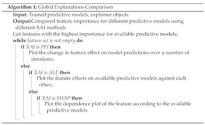
To compare the outcomes of all XAI methods we followed the steps illustrated in Algorithm 1. For PFI and SHAP methods, we study highly correlated features and their importance according to the XAI methods. In addition, we study how the applied model-agnostic XAI methods analyse the importance of features denoted as important to the predictive models through their model-specific explanations, i.e., coefficients in case of LR and features importance in case of XGBoost. In addition to the aforementioned comparisons, we compare the execution times for all applied XAI methods, including time for initiating the explainer and computing features importance as well. We included the training time of the predictive model as the execution time for model-specific methods.
Local Explainability Analysis
In this set of experiments, we apply two model-agnostic XAI methods, namely LIME [11] and SHAP [5], and analyse their outcomes separately. We apply variable and coefficient stability analysis [19] on LIME to study the stability of important feature sets and their coefficients across several runs.
5. Results and Observations
To validate our framework, we conducted experiments that use combinations of all choices available in each dimension. All experiments were run using Python 3.6 and the scikit-learn library [23] on a 96 core of a Intel(R) Xeon(R) Platinum 8268 @2.90 GHz with 768 GB of RAM. The code of executed experiments is available through our Github repository (https://github.com/GhadaElkhawaga/PPM_XAI_Comparison (accessed on 6 June 2022)) to enable open access for interested practitioners. It is important to view explanations in the light of all contributing factors, e.g., input characteristics, the effect of preprocessing inputs, and the way how certain predictive model characteristics affect its reasoning process. In [21], we study the effect of different input characteristics, preprocessing choices, and ML models characteristics and sensitivities on the resulting explanations. This section illustrates the observations we made during the experiments set out in Section 4. Due to lack of space, we focus on the most remarkable outputs illustrated by figures and tables. Further results can be generated by running the code of the experiments, which can be accessed via our Github repository. We believe that code publicity enables experiments replication and code reusability to introduce further improvements.
5.1. Global Methods Comparability
This subsection presents an analysis of PFI, ALE, and SHAP results. We execute two runs of each XAI method to query LR and XGBoost models trained over the event logs preprocessed with single aggregation and prefix index combination. Results are compared to get insights into their stability. Then, we follow the steps in Algorithm 1 to compare how each method highlighted the influence of the most important features (according to each predictive model) on predictions generation.
Permutation Feature Importance (PFI). The basic idea of PFI is to measure the average between the prediction error after and before permuting the values of a feature [4]. Each of the two PFI execution runs included 10 permutation iterations. The mean importance of each feature is computed. PFI execution led to the following observation:
Observation 1:In single-aggregated event logs, the results of the two runs are consistent with respect to feature sets and the weights of these features. In prefix-indexed event logs, the two runs are consistent in all event logs with exceptions in logs with longer prefixes.
An exception is present in prefix-indexed event logs derived from BPIC2017_Refused. In the latter event logs, the dissimilarity between the feature sets across the two runs increases with increasing length of the prefixes. This observation can be attributed to the effect of the increased dimensionality in the event logs with longer prefixes. For prefix-indexed event log, weights of important features change with increasing prefix length.
Accumulated Local Effects (ALE). ALE [12] calculates the change of the predictions as a result of changing the values of a feature, while taking features interactions into account [4]. This implies dividing feature values into quantiles [24] and calculating the differences in the predictions for feature values with a little shift above and below the feature value within a quantile. The described mechanism complicates calculating ALE effects for categorical features, especially one-hot encoded features. However, recently the common Python implementation of ALE was modified to compute ALE effects for one-hot encoded features using small values around 0 and 1 [24]. Despite the workaround, computing ALE effects for categorical attributes can be criticised for being inaccurate, as the values of these features do not maintain order [4,24], i.e., they are nominal features. As another issue, after running ALE over a given event log, effects of each feature are not in a form that yields a rank directly. Therefore, we ranked features based on the entropy of their computed effects.
While comparing two execution runs of ALE over the analysed event logs, we make the following observation:
Observation 2:The encoding technique applied plays a critical role with respect to (dis)similarity between feature ranks in the two execution runs. As an overall observation, ALE tends to be unstable over two runs.
In single-aggregated event logs, there is no similarity between the most influencing features in two execution runs. In contrast, in prefix-indexed event logs, this observation is not valid in all cases. For example, in prefix-indexed versions of all Sepsis logs, there is no similarity between features ranks in both execution runs. In turn, in Traffic_fines and BPIC_Refused encoded with the same combination, the top ranked features are categories derived from the same categorical attributes. Due to the inefficiency of ALE to compute effects of categorical attributes, we lean towards a conclusion that a rank, where categories derived from categorical attributes dominate, tends to be highly affected by collinearity between categories of such features. This conclusion is valid especially in event logs encoded with a technique that increases the number of categorical attributes exponentially, i.e., index encoding. In aggregation encoding, where results from two runs disagree, ranks tend to be more reliable. Aggregation encoding tends to increase the number of ordinal categorical attributes and preserve the existence of numerical attributes. Therefore, feature ranks of a single run tend to be less affected by collinearity. These observations are valid regardless of the underlying predictive model, which enables neutralising the effect of characteristics of the used predictive model.
SHapley Additive exPlanations (SHAP). SHAP is an explanation method belonging to the class of feature additive attribution methods [5]. These methods use a linear explanation model to compute the contribution of each feature to a change in the prediction outcome with respect to a baseline prediction. Afterwards, a summation of the contributions of all features approximates the prediction of the original model. To maintain comparability of the global XAI methods used in our experiments, we constructed a SHAP explainer model on training event logs independently of another SHAP explainer model constructed on relevant testing event logs. The concluded observations made in this section are drawn based on the training SHAP explainer model, whereas the observations based on the testing SHAP explainer model are discussed in Section 5.1.1 along with other observations concerning local XAI methods.
Observation 3:While comparing the two execution runs, results did not depend on the preprocessing technique used, but differed depending on the predictive model being explained.
When explaining predictions of the LR model, performing two executions of the SHAP method did neither result in different feature sets nor different ranks based on SHAP values, regardless the used preprocessing combination. In turn, explaining predictions of XGBoost model reveals the first most contributing feature as being the same across both execution runs, while the rest of the feature set is the same, but differs with respect to features’ ranks. An exception is present in the feature set of the three Sepsis event logs, where feature ranks are the same across both runs.
5.1.1. Comparability
Our study on how PFI, ALE and SHAP analysed the effects or contributions of the most important feature for each predictive model, led to some interesting observations:
Observation 4:The cardinality of categorical features has an effect on the explanations generated by permutation-based methods, which depend on measuring the prediction errors after changing a feature value. The effect of the used preprocessing combination depends on the used predictive model.
For features with lower number of categories, PFI is unable to capture the effect of shuffling feature values on predictions. The effect of shuffling a feature value is static in predictions generated using LR on most event logs, approaching zero in most cases. However, a slight change across PFI iterations can be observed in event logs preprocessed with single aggregation techniques. This observation indicates an effect of the encoding technique along with the interactions between the features. Shuffling values in PFI aims to break dependencies between the features [4]. However, with a low cardinality of a feature, the chances of reducing dependencies decreases over a few number of iterations.
PFI over XGBoost is presenting slightly higher shuffling effects in prefix-indexed event logs than in LR. This effect is slightly changing over shuffling iterations in the same event logs. However, the increase of changes in XGBoost predictions over iterations of shuffled feature values are observed in prefix-indexed event logs to be higher than in single-aggregated ones. Figure 3 shows PFI scores for the Traffic_fines event log, which was preprocessed with single aggregation (Figure 3(1-a),(2-a)) and prefix index (Figure 3(1-b),(2-b)). Figure 3(1-a),(1-b) represent change in prediction errors for both predictive models while changing the top important features to XGBoost. Finally, Figure 3(2-a),(2-b) represent the same for the top two important features to LR.
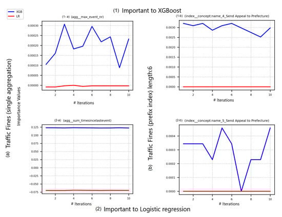
Figure 3.
PFI scores over Traffic_fines event log.
Dependence plots in SHAP represent an illustrative way presenting the effect of low cardinality in some features. These plots offer analyses of the effect of changing a feature’s values on SHAP values while taking the interaction effect of another feature into account. As opposed to PFI, this facility enables us to acquire more information from categorical features. For example, Figure 4 shows SHAP values of a feature CreditScore_other according to both XGBoost and LR predicting outcomes over BPIC2017_Refused event log preprocessed with single aggregation combination. Note that this feature is indicated as the most important one according to LR coefficients and as one of the top five important features based on the XGBoost gain criterion. This feature is a binary feature. However, it has multiple categorical levels due to being encoded based on its frequency of occurrence in a process instance. SHAP values of the feature form a nonlinear curve in XGBoost, and a linear one in LR. In both sub-figures, a point corresponds to a process instance. A point is colored according to its value of an interacting feature, which in this case is std_event_nr. According to LR, shap values increase linearly with increasing CreditScore_other values. The interacting feature values are increasing, as well. However, as a result of having all points of the same CreditScore_other value with identical shap value, it is unclear whether all points of the same CreditScore_other have the same std_event_nr value. In turn according to XGBoost, there is an interaction between both features resulting in having points with the same CreditScore_other value to obtain different shap values. These shap values decrease as the values of std_event_nr increase for points with the same CreditScore_other value.
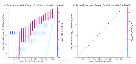
Figure 4.
SHAP Dependence plots of BPIC2017_Refused (single aggregation) event log.
Observation 5:In all event logs, ALE plots for LR are linear themselves.
An exception to this observation is present in the Traffic_fines event logs preprocessed with single aggregation. In Figure 5a, the importance of the feature sum_timesincelastevent, as indicated by LR coefficients, is confirmed by the change in ALE scores with a sudden decrease with increasing feature values. Although Figure 5 also shows a drecrease in XGBoost predictions, the expected decrease is stable and not steep after sum_timesincelastevent is reaching a value of (0.5 × 10⁶) unlike the case with LR model. However, in both cases ALE plot is interpolating as a result of the big gap in feature distribution. Note that the deciles on the x-axis represent interval edges at which ALE scores are calculated. In turn, in between the deciles are parts in which the ALE plot is interpolating. Absence of data might be an issue in non-linear models, where the ALE plot is interpolating and hence results might be unreliable in such regions.
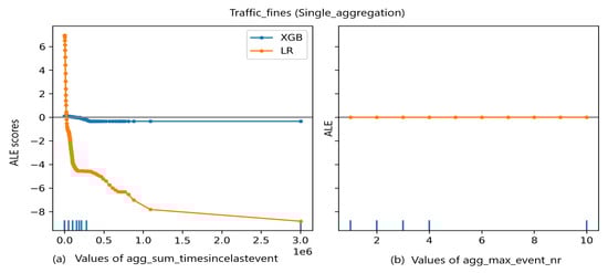
Figure 5.
ALE plot of Traffic_fines event log.
Observation 6:As expected, explaining how a predictive model uses a feature in predicting outcomes of an event log with class imbalance does not reveal a lot of information.
This observation is confirmed in results of the three XAI methods, especially when explaining LR reliance on important features. Results of event log Sepsis1 shown in Figure 6, Figure 7 and Figure 8 represent an example of this observation.
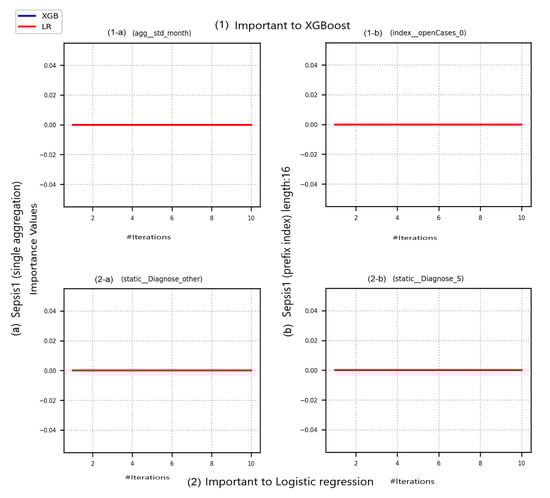
Figure 6.
PFI scores over Sepsis1 event log.
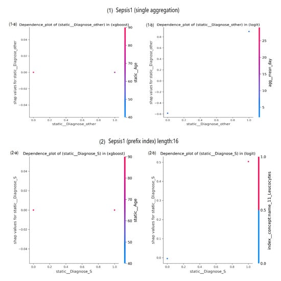
Figure 7.
SHAP Dependence plots of Sepsis1 event log.
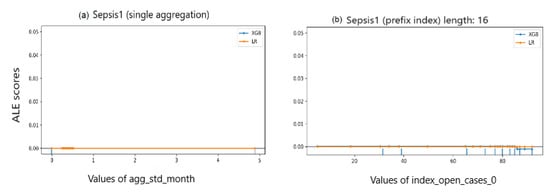
Figure 8.
ALE scores of Sepsis1 event log.
In Figure 6, despite the plotted features are indicated as important to the predictive models, after shuffling feature values over 10 iterations, there is no observed effect on the prediction error. In turn, in Figure 7(1-a),(2-a), the feature is showing no contribution to change in XGBoost predictions. This observation is represented by the zero SHAP values scored by the categorical features Diagnose_other (Figure 7(1-b)) and Diagnose_S (Figure 7(2-b)) in single-aggregated and prefix-indexed versions of Sepsis1, respectively. While a change is observed in LR predictions as a contribution of Diagnose_other in the single aggregation-encoded Sepsis1, without effect of the interaction with the feature mean_day. However, in Figure 7(2-b), there is an effect of the interaction between Diagnose_S and concept:name_11_Leucocytes. It is unclear whether this is the main affecting interaction, as all points with the same value of Diagnose_S provide the same contribution in terms of same SHAP values. ALE, as PFI and SHAP, is unable to reveal more information about Sepsis1. In Figure 8, both predictive models are not affected by changes in analysed features values, despite being highlighted as the most important features. In both sub-figures, the ALE plot is linearly interpolating in between available data. However, in both sub-figures ALE scores are nearly zero.
As an example, consider the global analysis of BPIC2017_Accepted event log, which is shown in Figure 9, Figure 10 and Figure 11. The high cardinality of the analysed features along with the high number of process instances expose the effect of value change on LR predictions, especially using PFI as shown in Figure 9. The same factors are affecting important features to XGBoost using SHAP and ALE as shown in Figure 10 and Figure 11, especially with ALE where the plot is less interpolating with more dispersion of data. In SHAP dependence plots, SHAP values are following a non-linear form, while the interaction effect is clear even in std_MonthlyCost feature which is more important to LR than XGBoost.
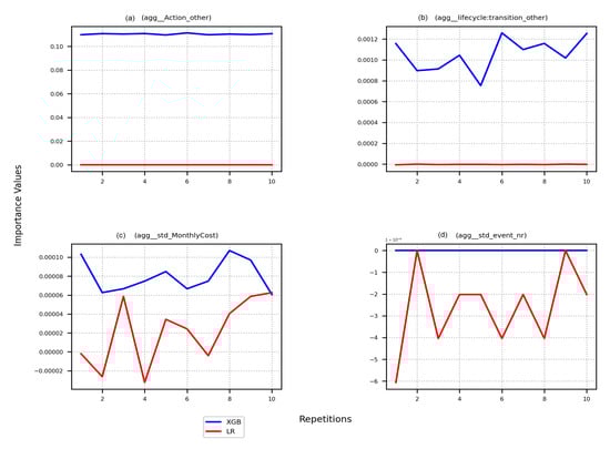
Figure 9.
PFI scores of BPIC2017_Accepted event log.
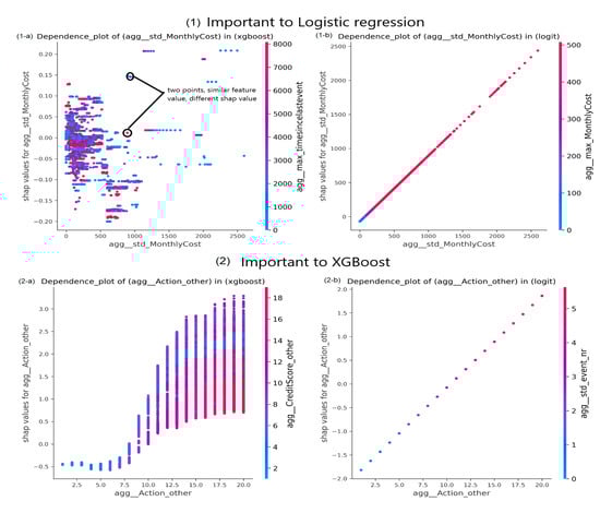
Figure 10.
SHAP Dependence plots of BPIC2017_Accepted event log.
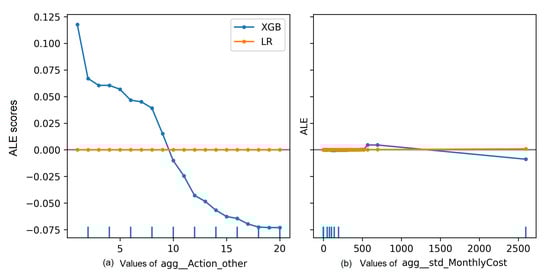
Figure 11.
ALE scores of BPIC2017_Accepted event log.
5.1.2. Execution Times
For applied XAI methods, the execution times are computed for SHAP, ALE and PFI over the training event logs. Prediction times of LR and XGBoost are included as the time for computing the importance of the features to the predictive models. Execution times are presented in Table 3 and Table 4. More precisely, the execution times of event logs preprocessed with single aggregation and prefix index combination respectively are displayed. Note that in the event log column in Table 4, each event log is augmented with the length of its prefixes.
Table 3.
Execution times (in seconds) of XAI methods on event logs preprocessed using single aggregation combination.
Table 4.
Execution times (in seconds) of XAI methods on event logs preprocessed using prefix index combination.
In terms of the underlying preprocessing technique, the overall numbers across all XAI methods show that event logs preprocessed with prefix index combination are faster to be explained than those preprocessed with single aggregation.
Observation 7:We conclude that the chosen bucketing technique is a determinant factor affecting execution duration of global explanations generation.
As illustrated by [2,3], in index encoding, with increasing prefix length, the number of features increases, while the number of process instances decreases in an event log. The reduced number of process instances in a prefix index-preprocessed event log compared to a single-aggregated event log can justify the faster execution times on the former logs. Despite enabling faster executions, as expected, prefix-indexed event logs with longer prefixes show longer execution times over all XAI methods than event logs with shorter prefixes.
Observation 8:The overall numbers show that explaining decisions of a LR model takes less time compared to the use of an XGBoost-based model.
This observation has provedn to be true when regarding the results across different event log sizes and preprocessing settings as well as over different XAI methods. A justification of this observation may be that all studied global XAI methods involve querying the underlying model. The boosting mechanism employed in XGBoost complicates the prediction process, and hence it demands more time to produce predictions or, subsequently, explanations.
Observation 9:When regarding execution times of different XAI methods, it can be observed that SHAP has the fastest executions over almost all event logs, regardless the used preprocessing techniques (with few exceptions).
An exception to this observation is the execution time of SHAP over the shortest prefix version of Traffic_fines event log being preprocessed with prefix index combination and having an XGBoost model trained over its process instances. SHAP values for this event log are the slowest among all XAI methods.
Observation 10:The slowest XAI method differs based on the preprocessing techniques used, with ALE performing worst in most cases.
In prefix-indexed event logs, PFI achieves the worst performance for most event logs when combining it with LR, and ALE shown the worst performance in combination with XGBoost. In turn, in single aggregation-based event logs, ALE provides the least efficient XAI method to be combined with either predictive models. PFI performs worst in smaller event logs with relevant small numbers of features compared to other logs, e.g., in the three Sepsis event logs. Figure A1 and Figure A2 in Appendix A provide a visualisation of the execution times of XAI methods on event logs using prefix index and single aggregation preprocessing combinations, respectively.
5.2. Local Methods Comparability
LIME and SHAP, which are the two local XAI methods used in this study, share the underlying mechanism. Both are feature additive attribution methods [5]. LIME is looking for the weights of features in order to indicate their importance, While SHAP calculates contributions of features to shifting the current process instance prediction towards or apart from a base prediction. To gain insights into how LIME and SHAP results can differ while explaining the same process instances, we compared their explanations of both predictive models reasoning, i.e., LR and XGBoost, over a selected set of process instances from each event log preprocessed with both preprocessing combinations. After analysing the resulting explanations, the following observations can be made:
Observation 11:It could be rarely observed when both methods match in their attributions to important features or in the strength and direction of the effect features have on driving the current prediction towards or away from the base prediction.
It is supposed that whenever both XAI methods explain the prediction generated by the same predictive model for the same process instance, a similarity between the explanations exists. However, the former observation is valid across all event logs regardless the preprocessing combinations used. If both methods agree on a subset of features, they do not have the same importance ranks. Note that in LIME the goal is to identify a set of features which are important in confirming the current prediction or driving the prediction towards the other class in case of binary classification tasks. In turn in SHAP the purpose is to order features descending based on their SHAP values, i.e., their contributions in driving the current prediction away or towards the base prediction over the whole event log. As example consider the two explanations from Figure 12, which shows the LIME explanation (cf. Figure 12a) and the SHAP decision plot (cf. Figure 12b) of prediction made by LR of the same process instance of Traffic_fines event log preprocessed with prefix index. In Figure 12a, important features are listed in descending order along with their values in the event log based on the coefficients of these features in the approximating model created by LIME. On the bottom of Figure 12a, again these features are listed with the percentage of their contributions. Note that the color code of these features represents whether a feature is driving the prediction towards the currently predicted class or towards the other class. In this case, the currently predicted class is “deviant”.
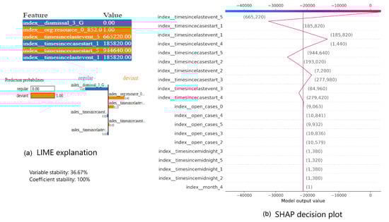
Figure 12.
LIME vs. SHAP explanations of LR prediction for one instance in Traffic_fines preprocessed with prefix index combination.
Figure 12b shows the decision plot highlighting the features with the highest shap values in descending order. The line at the center represents the base prediction or model output. The zigzag line represents the current prediction and stricks the top at exactly the current prediction value. Prediction units are in log odds. The pattern at which the zigzag line is going towards and outwards from the line at the center represents contributions of features at the y-axis to reducing/increasing the difference between the base and current predictions. In addition, feature values are stated in brackets over the zigzag line at the point where the line intersects with the horizontal line. It can be observed that the decision plot is indicating that the current prediction of the LR model is highly affected by collinear features.
Observation 12:In explanations of both methods, dynamic attributes are dominating feature sets.
This observation about the explanations can be justified by having all event logs, except for the three dervied from Sepsis event log, with a larger number of static attributes and a relatively lower number of dynamic ones (cf. Table 1). Therefore as expected, dynamic attributes are dominating feature sets provided by local explanations. This observation may be justified by the fact that both employed encoding techniques are able to increase the number of features derived from dynamic ones, especially in event logs for which the dynamic features dominate.
Another example of an explanation is presented in Figure 13. It shows LIME (Figure 13a) and SHAP (cf. Figure 13b) explanations of a prediction generated by an XGBoost model for a process instance of the BPIC2017_Cancelled event log while being preprocessed with single aggregation combination. In both explanations, CreditScore_other is the most or second important feature. In LIME, this feature is the only one driving the prediction towards the currently predicted class. Meanwhile in SHAP, the same feature has the highest SHAP value that drives the current prediction away from the base prediction. This means that this feature has the highest impact according to both explanations.
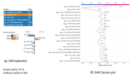
Figure 13.
LIME vs. SHAP explanations of XGBoost prediction for one process instance in BPIC2017_Cancelled preprocessed with single aggregation combination.
As mentioned in Section 4.1, stability measures, namely Variable Stability Index (VSI) and Coefficient Stability Index (CSI), are applied on LIME explanations. VSI [19] measures to what extent the same set of important features will be generated if LIME is executed several times over the same event log under the same conditions. In turn, CSI [19] measures the stability in coefficients of features within the important feature set over several runs of LIME.
Observation 13.1:For the randomly selected process instances from different event logs, as expected, Variable Stability Index (VSI) shows high instability in LIME explanations over several runs.
This observation can be justified by the high dimensionality of the analysed event logs. According to [19], the underlying approximating model used by LIME, fits the generated dataset based on multivariate distribution of features in the original dataset. The original model is queried for labels of the newly generated dataset. Afterwards, the distance between the newly generated data points and the sample to be explained is measured. In case of high dimensionality, it is not possible to distinguish between distant and near points. The latter phenomena will result in generating a dataset that will differ greatly from the explained sample. As a result, the approximating model is expected to be locally inaccurate compared to the original model [5,19], besides having a different approximating model at each LIME run. Consequently, different feature sets will result whenever querying the approximating model.
Observation 13.2:The VSI of LIME explanations of XGBoost predictions is higher in balanced event logs. In case of LIME explanations of LR predictions, it is higher in imbalanced event logs.
For example, the VSI of the explanation of the instance in Figure 13 is 93.7%.
Observation 13.3:CSI measures are high for LIME explanations of XGBoost predictions for all event logs, whereas the same measures are zeros for the explanations of the predictions by LR on almost all imbalanced event logs.
This observation can be justified by the underlying collinearity of data and sensitivity of linear models (in this case the approximating linear model) to such phenomena. Consequently, the approximating model is expected to assign unstable coefficients to collinear features at each run of LIME. Therefore, CSI measures are unstable.
6. Discussion
Explaining ML-based predictions becomes necessity to gain user acceptance and trust in the predictions of any predictive models. We need to consider explainability as a continuous process that should be integrated throughout the entire ML pipeline. A first step towards such integration would be a study of the effect of different pipeline decisions on the resulting explanations. Our main concern in this research is to study the ability of an explanation to reflect how a predictive model is affected by different settings in the ML pipeline. The experimental results described and analysed in Section 5 confirm the following conclusions:
- Both studied encoding techniques load the event log with a large number of derived features. However, the situation becomes worse in index-based encoding, as the number of resulting features is increasing proportionally to the number of dynamic attributes, especially the number of categorical levels of a dynamic categorical attribute. Dimensionality explosion has an effect on the explanations generated in the same way it has on predictions generation. On one hand, explaining high-dimensional event logs becomes expensive in terms of computational resources, especially in XAI methods that run multiple iterations to rank features based on their importance, for example in case of PFI. We denote this as the horizontal effect of dimensionality. Furthermore, other XAI methods can not work on lower cardinality features, (e.g., ALE), or can work on it but will not yield useful insights. A high dimensional event log may hold non-useful features that may have been used by the predictive model. However, it cannot be used to explain the prediction generated. We denote this as the vertical effect of dimensionality. However, SHAP is the only XAI method among the compared ones that is able to mitigate the effect of lower cardinality and to produce meaningful explanations while highlighting the effect of interactions between analysed features in dependency plots. These effects are observed in explanations of process instances from the preprocessed event logs using index encoding more than aggregation-based preprocessed event logs.
- Increased collinearity in the underlying data is another problem resulting from encoding techniques with varying degrees. The effect of collinearity can be observed in index-based preprocessed event logs, while not being completely absent in aggregation-based event logs. This collinearity is reflected through explanations of predictions on process instances from prefix-indexed event logs as the length of a prefix increases. Another effect of collinearity is the instability of LIME explanations. This instability is due to the approximating model affected by collinear features (in terms of unstable feature coefficients) and high dimensionality (in terms of unstable feature sets).
- PFI showed to be more stable and consistent along two execution runs, while SHAP stability is affected by the underlying predictive model while may be (in)sensitive to the underlying data characteristics. ALE is mostly unstable and affected by its inability to accurately analyse effects of changes in categorical attributes on predictions generated.
Observations made in the context of this study raise potential opportunities for further research. Setting criteria for evaluating XAI methods is a demanding need to ensure acceptance and trustworthiness of the XAI methods themselves. Measurements should be put in place to ensure stability and replicability of results across several runs of an XAI method. Sensitivity of an XAI method to changes in underlying data or underlying predictive model should be measured and an XAI method should be evaluated for. This issue highlights the need to regard an explainability method as an optimisation problem where different underlying choices affect the final outcome, as proven by the results of our study.
7. Related Work
Some work available from related research areas is considered complementary to the work we present in this paper. These research efforts enabled us to gain a solid understanding of how different aspects of predictions explainability are studied in the context of PPM, besides shedding light on possible research gaps.
7.1. Leveraging PPM with Explanations
The authors of [25] propose an approach that integrates Layer-wise Relevance Propagation (LRP) to explain the next activity predicted with an LSTM predictive model. This approach tends to propagate relevance scores backwards through the model to indicate which previous activities were crucial to obtaining the resulting prediction. This approach provides explanations for single predictions, i.e, local explanations.
Another approach explaining an LSTM decisions is present in [26]. However, in [26], the authors claim that the approach is model-agnostic and independent from the chosen predictive model. This approach predicts the execution of certain activities, besides predicting remaining time and cost of a running process instance. The total number of process instances where a certain feature is contributing either positively or negatively to a prediction is identified at each timestamp for the whole dataset. This identification is directed by SHAP values. The authors of [26] use the same approach in providing local explanations for running process instances.
Explanations can be also used to leverage a predictive model performance as proposed by [27]. Using LIME as a post-hoc explanation technique to explain the predictions generated with Random Forest, In [27], the authors identify feature sets that contributed to produce wrong predictions. After identifying these feature sets, their values are randomised, provided that they do not contribute to generating right predictions for other process instances. The resulting randomised dataset is then used to retrain the model again till its perceived accuracy becomes improved.
7.2. Using Transparent Models in PPM Tasks
The proposals by [28,29] represent attempts to provide a transparent PPM approach, supported by explanation techniques with the aim of providing a transparent predictive model. In [29], the authors conduct experiments on three different predictive models to predict the next activity only using control-flow information, the next activity supported with dynamic attributes, and the next activity along with remaining time. The authors of [29] use LSTM with attention mechanisms to provide attention values indicating attention weights used to direct the attention of the predictive model to certain features. According to [30,31], there is a lot of work in the field of Natural Language processing (NLP) about whether to use attention weights as explanations, as attention weights are not always correlated to feature importance [30].
In [28], the authors propose a process-aware PPM approach to predict the remaining time of a running process instance, while providing a transparent model. However, the authors of [28] could not prove that the proposed approach provides comprehensible explanations from the user perspective. In turn, the proposed approach includes discovering a process model, training a set of classifiers to provide probabilities of gates in the discovered process model, and training a set of regressors to perform the main prediction task. These procedures are a source of computation overhead, which is not confirmed or disproved by [28].
8. Conclusions
In this research, a framework has been proposed that enables comparing explanations generated by a selected number of currently available XAI methods. The XAI methods under analysis explain decisions of ML models generating predictions in the context of PPM. Our study includes a comparison of the XAI methods at different granularity levels (global and local XAI), given different underlying PPM workflow decisions with respect to data, preprocessing, and chosen models. A study of how an XAI method is able to reflect the sensitivity of a predictive model towards underlying data characteristics is provided. In turn, different XAI methods are compared according to different criteria including stability and execution duration, over different granularities, i.e., globally and locally.
This study has revealed how explanations can highlight data problems through analysing the model reasoning process. For example, we have uncovered issues resulting from collinearity between features, while having this collinearity being the product of characteristics of the chosen preprocessing combination of techniques. It has further emphasized based on experiments, the importance of feature selection after preprocessing an event log. We have emphasized the effect of an XAI method vulnerabilities on the quality of information provided by its relevant generated explanations, e.g., in the case of ALE. Using our comparative framework, we highlighted the power of SHAP to unleash important information about relation between features and also their impact on the target. This conclusion is highlighted using experiments on SHAP in comparison to other XAI methods, using its global and local method versions. Based on our experiments and results, the phrase “garbage-in garbage-out” is not just valid in the case of predicting using machine learning models, but also applies to explaining these predictions. It was proved whenever predictions on imbalanced data are explained. Our study has highlighted situations where data problems might not affect the accuracy of predictions, but do affect usefulness and meaningfulness of explanations. Explainability should be seamlessly integrated into PPM workflow stages as an inherent task not as a follow up effort.
Author Contributions
G.E.-k. drafted and revised the manuscript. G.E.-k. was responsible for conceptualizing this work. G.E.-k. was responsible for the formal analysis, methodology, and writing the original draft. M.R. was responsible for reviewing and editing this article. M.A.-E. and M.R. validated and supervised this work. M.R. was responsible for funding acquisition. All authors have read and agreed to the published version of the manuscript.
Funding
This study is carried out through fund provided as part of the cognitive computing in socio-technical systems program granted to the last author as the supervisor of the first author as a PhD candidate.
Institutional Review Board Statement
Not applicable.
Informed Consent Statement
Not applicable.
Data Availability Statement
Datasets used in the context of our experiments are available at 4TU Centre for Research Data: https://data.4tu.nl/Eindhoven_University_of_Technology (accessed on 6 June 2022) and the code is accessible through https://github.com/GhadaElkhawaga/PPM_XAI_Comparison (accessed on 6 June 2022).
Conflicts of Interest
The authors declare no conflict of interests.
Abbreviations
The following abbreviations are used in this manuscript:
| ML | Machine Learning |
| PPM | Predictive Process Monitoring |
| XAI | eXplainable Artificial Intelligence |
| GAM | General Additive Model |
| RQ | Research Question |
| MI | Mutual Information |
| LR | Logistic Regression |
| PFI | Permutation Feature Importance |
| PDP | Partial Dependence Plots |
| ALE | Accumulated Local Effects |
| SHAP | SHapley Additive exPlanations |
| VSI | Variable Stability Index |
| CSI | Coefficient Stability Index |
| LRP | Layer-wise Relevance Propagation |
Appendix A
This appendix reports the following:
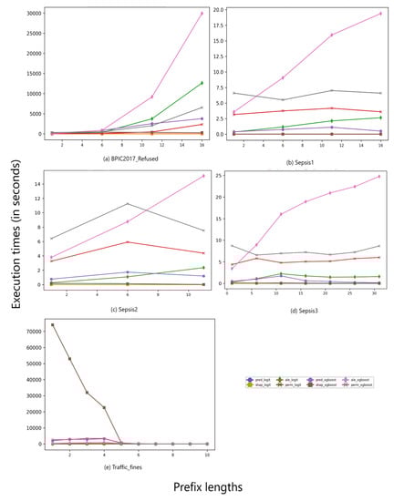
Figure A1.
Execution times (in seconds) of XAI methods on event logs preprocessed using prefix index combination.
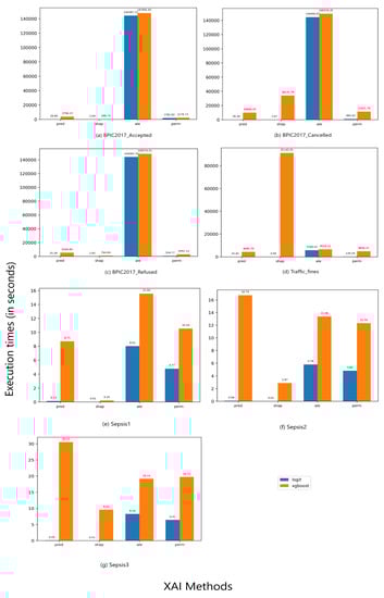
Figure A2.
Execution times (in seconds) of XAI methods on event logs preprocessed using single aggregation combination.
References
- Van der Aalst, W. Process Mining: Data Science in Action, 2nd ed.; Springer: Berlin/Heidelberg, Germany, 2016. [Google Scholar]
- Verenich, I.; Dumas, M.; Rosa, M.L.; Maggi, F.M.; Teinemaa, I. Survey and Cross-benchmark Comparison of Remaining Time Prediction Methods in Business Process Monitoring. ACM Trans. Intell. Syst. Technol. 2019, 10, 34. [Google Scholar] [CrossRef] [Green Version]
- Teinemaa, I.; Dumas, M.; Rosa, M.L.; Maggi, F.M. Outcome-Oriented Predictive Process Monitoring: Review and Benchmark. ACM Trans. Knowl. Discov. Data 2019, 13, 57. [Google Scholar] [CrossRef]
- Molnar, Christoph: Interpretable Machine Learning: A Guide for Making Black Box Models Explainable. 2019. Available online: https://christophm.github.io/interpretable-ml-book/ (accessed on 6 June 2022).
- Lundberg, S.; Lee, S. A unified approach to interpreting model predictions. In Proceedings of the 31st International Conference on Neural Information Processing Systems, Long Beach, CA, USA, 4–9 December 2017; pp. 4768–4777. [Google Scholar]
- Friedman, J.H. Greedy function approximation: A gradient boosting machine. Ann. Statist. 2001, 29, 1189–1232. [Google Scholar] [CrossRef]
- Shrikumar, A.; Greenside, P.; Kundaje, A. Learning important features through propagating activation differences. In Proceedings of the 34th International Conference on Machine Learning, Sydney, Australia, 6–11 August 2017; pp. 145–3153. [Google Scholar]
- Binder, A.; Montavon, G.; Lapuschkin, S.; Müller, K.R.; Samek, W. Layer-Wise Relevance Propagation for Neural Networks with Local Renormalization Layers. In Artificial Neural Networks and Machine Learning—ICANN; Villa, A., Masulli, P., Rivero, A.J.P., Eds.; Springer: Cham, Switzerland, 2016; Volume 9887, pp. 63–71. [Google Scholar]
- Wachter, S.; Mittelstadt, B.; Russell, C. Counterfactual Explanations without Opening the Black Box: Automated Decisions and the GDPR. Harv. J. Law Technol. 2018, 31, 841. [Google Scholar] [CrossRef] [Green Version]
- Kindermans, P.J.; Hooker, S.; Adebayo, J.; Alber, M.; Schütt, K.T.; Dähne, S.; Erhan, D.; Kim, B. The (Un)reliability of Saliency Methods. In Explainable AI: Interpreting, Explaining and Visualizing Deep Learning; Samek, W., Montavon, G., Vedaldi, A., Hansen, L.K., Müller, K., Eds.; Springer: Cham, Switzerland, 2019; Volume 11700, pp. 267–280. [Google Scholar]
- Ribeiro, M.T.; Singh, S.; Guestrin, C. Why Should I Trust You? In Proceedings of the 22nd ACM SIGKDD International Conference on Knowledge Discovery and Data Mining, San Francisco, CA, USA, 13–17 August 2016; pp. 1135–1144. [Google Scholar]
- Apley, D.W.; Zhu, J. Visualizing the effects of predictor variables in black box supervised learning models. J. R. Stat. Soc. 2020, 82, 1059–1086. [Google Scholar] [CrossRef]
- Doshi-Velez, F.; Kortz, M. Accountability of AI under the Law: The Role of Explanation, Berkman Klein Center Working Group on Explanation and the Law, Berkman Klein Center for Internet & Society Working Paper. 2017. Available online: http://nrs.harvard.edu/urn-3:HUL.InstRepos:34372584 (accessed on 6 June 2022).
- Arrieta, A.B.; Díaz-Rodriguez, N.; Del Ser, J.; Bennetot, A.; Tabik, S.; Barbado, A.; Garcia, S.; Gil-López, S.; Molina, D.; Benjamins, R.; et al. Explainable Artificial Intelligence (XAI): Concepts, taxonomies, opportunities and challenges toward responsible AI. Inf. Fusion 2020, 58, 82–115. [Google Scholar] [CrossRef] [Green Version]
- Mohseni, S.; Zarei, N.; Ragan, E.D. A Multidisciplinary Survey and Framework for Design and Evaluation of Explainable AI Systems. ACM Trans. Interact. Intell. Syst. 2021, 11, 1–45. [Google Scholar] [CrossRef]
- Zhou, J.; Gandomi, A.H.; Chen, F.; Holzinger, A. Evaluating the Quality of Machine Learning Explanations: A Survey on Methods and Metrics. Electronics 2021, 10, 593. [Google Scholar] [CrossRef]
- Guidotti, R.; Monreale, A.; Ruggieri, S.; Turini, F.; Giannotti, F.; Pedreschi, D. A Survey of Methods for Explaining Black Box Models. ACM Comput. Surv. 2019, 51, 1–42. [Google Scholar] [CrossRef] [Green Version]
- Nguyen, A.; Martínez, M.R. On Quantitative Aspects of Model Interpretability. 2020. Available online: http://arxiv.org/pdf/2007.07584v1 (accessed on 6 June 2022).
- Visani, G.; Bagli, E.; Chesani, F.; Poluzzi, A.; Capuzzo, D. Statistical stability indices for LIME: Obtaining reliable explanations for machine learning models. J. Oper. Res. Soc. 2021, 12, 1–11. [Google Scholar] [CrossRef]
- Outcome-Oriented Predictive Process Monitoring Benchmark- Github. Available online: https://github.com/irhete/predictive-monitoring-benchmark (accessed on 26 April 2022).
- Elkhawaga, G.; Abuelkheir, M.; Reichert, M. Explainability of Predictive Process Monitoring Results: Can You See My Data Issues? arXiv 2022, arXiv:2202.08041. [Google Scholar]
- 4TU Centre for Research Data. Available online: https://data.4tu.nl/Eindhoven_University_of_Technology (accessed on 26 April 2022).
- Pedregosa, F.; Varoquaux, G.; Gramfort, A.; Michel, V.; Thirion, B.; Grisel, O.; Blondel, M.; Prettenhofer, P.; Weiss, R.; Dubourg, V.; et al. Scikit-learn: Machine Learning in Python. J. Mach. Learn. Res. 2011, 12, 2825–2830. [Google Scholar]
- Alibi Explain. Available online: https://github.com/SeldonIO/alibi (accessed on 26 April 2022).
- Weinzierl, S.; Zilker, S.; Brunk, J.; Revoredo, K.; Matzner, M.; Becker, J. XNAP: Making LSTM-Based Next Activity Predictions Explainable by Using LRP. In Business Process Management Workshops: International Publishing (Lecture Notes in Business Information Processing); Ortega, A.D.R., Leopold, H., Santoro, F.M., Eds.; Springer: Cham, Switzerland, 2020; Volume 397, pp. 129–141. [Google Scholar]
- Galanti, R.; Coma-Puig, B.; de Leoni, M.; Carmona, J.; Navarin, N. Explainable Predictive Process Monitoring. In Proceedings of the 2nd International Conference on Process Mining (ICPM), Padua, Italy, 4–9 October 2020; pp. 1–8. [Google Scholar]
- Rizzi, W.; Di Francescomarino, C.; Maggi, F.M. Explainability in Predictive Process Monitoring: When Understanding Helps Improving. In Business Process Management Forum: Lecture Notes in Business Information Processing; Fahland, D., Ghidini, C., Becker, J., Dumas, M., Eds.; Springer: Cham, Switzerland, 2020; Volume 392, pp. 141–158. [Google Scholar]
- Verenich, I.; Dumas, M.; La Rosa, M.; Nguyen, H. Predicting process performance: A white-box approach based on process models. J. Softw. Evol. Proc. 2019, 31, 26. [Google Scholar] [CrossRef] [Green Version]
- Sindhgatta, R.; Moreira, C.; Ouyang, C.; Barros, A. Exploring Interpretable Predictive Models for Business Processes. In Business Process Management, LNCS; Fahland, D., Ghidini, C., Becker, J., Dumas, M., Eds.; Springer: Cham, Switzerland, 2020; Volume 12168, pp. 257–272. [Google Scholar]
- Jain, S.; Wallace, B.C. Attention is not explanation. In Proceedings of the 2019 Conference of the North American Chapter of the Association for Computational Linguistics: Human Language Technologies, Minneapolis, MN, USA, 3–5 June 2019; pp. 3543–3556. [Google Scholar]
- Wiegreffe, S.; Pinter, Y. Attention is not not Explanation. In Proceedings of the 2019 Conference on Empirical Methods in Natural Language Processing and the 9th International Joint Conference on Natural Language Processing, Hong Kong, China, 3–7 November 2019; pp. 11–20. [Google Scholar]
Publisher’s Note: MDPI stays neutral with regard to jurisdictional claims in published maps and institutional affiliations. |
© 2022 by the authors. Licensee MDPI, Basel, Switzerland. This article is an open access article distributed under the terms and conditions of the Creative Commons Attribution (CC BY) license (https://creativecommons.org/licenses/by/4.0/).