Abstract
The group sparse representation (GSR) model combines local sparsity and nonlocal similarity in image processing, and achieves excellent results. However, the traditional GSR model and all subsequent improved GSR models convert the RGB space of the image to YCbCr space, and only extract the Y (luminance) channel of YCbCr space to change the color image to a gray image for processing. As a result, the image processing process cannot be loyal to each color channel, so the repair effect is not ideal. A new group sparse representation model based on multi-color channels is proposed in this paper. The model processes R, G and B color channels simultaneously when processing color images rather than processing a single color channel and then combining the results of different channels. The proposed multi-color-channels-based GSR model is compared with state-of-the-art methods. The experimental contrast results show that the proposed model is an effective method and can obtain good results in terms of objective quantitative metrics and subjective visual effects.
1. Introduction
Image restoration is one of the fundamental tasks in image processing and computer vision, and it aims to recover the original image from the observed degraded image . Image restoration is an ill-posed inverse problem and can be chartered by the following Formula (1):
Here, and represent the original image and the degraded image respectively, denotes the degenerate operator, and denotes additive Gaussian noise. is modeled according to different image processing tasks. When is a unit matrix, Formula (1) represents an image denoising task [1,2]. When is a blurring operator, Formula (1) represents an image deblurring task [3]. When is a mask, Formula (1) represents image restoration [4,5]. When is a random projection matrix, Formula (1) represents image compressive sensing applications [6,7].
The image restoration task is studied in this paper. In order to overcome the ill-posed characteristic and recover a satisfied copy of the original image, image priors are used to regularize the minimal problem,
where the first term represent the data fidelity term, represents the regularization term of the image a priori, and is a regularization parameter. Image priors play an important role in image restoration, and many relevant algorithms are proposed, such as total-variation-based methods [8,9,10], sparse-representation-based methods [11,12,13,14], nonlocal self-similarity-based methods [1,2,15] and deep-convolutional-neural-network-based methods [16,17,18].
Sparse representation is an effective technique in image processing. Sparse-representation-based algorithms can be divided into two categories, i.e., patch sparse representation (PSR) [11,19] and group sparse representation (GSR) [12,13,15]. In the PSR model, the basic sparse representation unit is the image block. PSR assumes that each block of the image to be repaired can be perfectly modeled by a sparse linear combination of some fixed or learnable basic elements. These basic elements are called atoms and constitute a set called a dictionary. The PSR model not only does well in image denoising [20], but also can be applied to various other image processing and computer vision tasks [21]. However, the PSR model with an over-complete dictionary usually produces visual artifacts which are not expected in image restoration [22]. In addition, the PSR model assumes that the coded image blocks using sparse representation are independent and ignores the correlation among similar image blocks [13,23], which results in image degradation. To solve the above problems, the GSR model uses an image group as its basic processing unit to integrate the local sparsity with the nonlocal self-similarity of images. GSR shows great potential in various image processing tasks, and many literatures are provided. Zhang et al. [13] proposed the traditional GSR model for image restoration, which is essentially equal to the low rank minimization model [24]. Dong et al. [25] proposed an effective Gaussian scale mixing-based image restoration model under the GSR framework. Zha et al. [26] proposed a group-based adaptive dictionary, which connects the GSR model with the low rank minimization model. Zha et al. [14] combined the PSR and GSR models to reduce their shortcomings, respectively. Zha et al. [27] introduced the group sparse residual constraints to the GSR model to further define and simplify the problem of image restoration.
The traditional GSR model and the improved GSR models usually transform the RGB space of the image into YCbCr space and extract the Y (luminance) component for image processing. The Y channel in YCbCr space contains much valuable information about edge, shadow, object, texture and others. Moreover, human vision is sensitive to the change of the Y channel. These good characteristics make the GSR model and its improved models very successful in various image processing tasks. However, these methods only extract the Y channel, and cannot be loyal to each color channel of the color image. In this paper, the color channels refer to red (R), green (G), and blue (B) channels in RGB space. In order to exploit all the three channels, we propose a new GSR model based on multi-color channels. Compared with the traditional GSR model, which only extracts the Y channel in YCbCr space, the proposed model preserves as much image information as possible.
The main contribution of the paper is to propose the multi-color-channels-based GSR model for image restoration. In this proposed model, three channels are exploited simultaneously, and hence as much image color information as possible is retained. The paper is organized as follows. Section 1 introduces briefly the image restoration models and the development of the sparse-representation-based methods. Section 2 describes the traditional GSR model. The proposed multi-color-channels-based GSR model is provided in Section 3. Section 4 provides the visual and quantitative experimental results. Finally, conclusions are given in Section 5.
2. GSP Model
Compared with the patch sparse representation (PSR) model, the traditional group sparse representation (GSR) model uses the image group instead of a single image block as the basic unit of sparse representation, which produces satisfactory results in image processing tasks [13,28,29]. The model proposed in this paper is based on the traditional GSR model, which is briefly introduced here.
2.1. Image Group Construction
The construction of the image group in GSR model is illustrated in Figure 1. The image with the size of is divided into overlapped patches with the size of . The overlapped patches are denoted by where . For each , its similar matched patches are constructed using the Euclidean distance as the similarity metric in a training window with the size of . The similar matched patches form a set denoted by . All the similar patches in form a matrix with the size of , denoted by . Each element in is a column of the matrix , i.e., . The column denotes the jth similar patch of the ith image group corresponding to . The matrix includes all the similar patches as columns, and hence is referred to as a group.
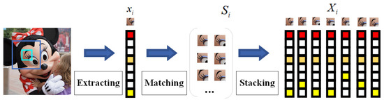
Figure 1.
The construction diagram of the image group.
2.2. Sparse Representation Model
After constructing the image group, a sparse representation model is established in the image group. In order to obtain the sparse representation model of the image group, a dictionary, denoted by is given, which is usually learned from the image group, such as the graph-based dictionary [30] and principal component analysis (PCA) dictionary [31]. The aim of the sparse representation is to present the image group using as few atoms of the dictionary as possible. That is, the task is to code the dictionary sparsely using a sufficiently sparse vector. Each sparse representation, denoted by , corresponding to the image group , is obtained via minimizing the norm using the following Formula (3).
Here, denotes the group sparse coefficient corresponding to the ith image group . is the fitting term used to measure the similarity between the image to be repaired via the sparse representation model and the original image. is a regularization parameter, and denotes the norm used to calculate the no-zero terms of each column in . Since norm minimization is NP-hard, norm minimization is used instead of norm minimization via the following Formula (4).
The original image is not available in the image restoration task, and the image groups are from the degraded image . The image is segmented into overlapped patches with the same size of , i.e., a vector with the length of . The similar matched patches are found to generate the image groups corresponding to the overlapped patches. Each image group denoted by is a matrix with the size of , which also can be written as . Now, the image restoration task is to restore from using the GSR model via the following Formula (5).
After obtaining , , the restored whole image can be represented by a set of sparse codes .
2.3. Learning a Dictionary
Sparse representation aims to obtain the sparsest representation of the original signal on the learned dictionary, and the signal is represented as a linear combination of a small number of dictionary atoms [32]. Therefore, in the framework of sparse representation, the construction of the dictionary is the key step of image restoration. However, in image restoration tasks, the original image is unknown, and the original image group cannot be obtained directly. The dictionary is only constructed according to the degraded image . The image is first initialized using the bilinear interpolation algorithm. The following operations are similar to the procedures depicted in Section 2.1. Specifically, the estimated image group corresponding to the original image group is extracted from the initialized image . Then the singular value decomposition is performed on the estimation group via the following Equation (6).
Here, denotes , denotes a diagonal matrix, denotes the main diagonal elements of , represents each atom of the dictionary , and is defined as the minimum of and . and denotes the column vectors of the matrixes and , respectively. Each atom of the adaptive dictionary is defined as follows,
In this way, the adaptive dictionary , corresponding to each image group can be represented as follows:
The singular value decomposition is only needed to be performed on each group once to learn the adaptive dictionary corresponding to the image group. After the dictionary is learned, the sparse representation model is updated and then the norm minimization is solved. Finally, the split Bregman iteration (SBI) algorithm [13] is used for iterative optimization to obtain the final restoration result.
3. Proposed Multi-Color Channels Based GSR Model
The image restoration algorithm based on the GSR model has achieved good results in applications. However, most image restoration algorithms based on the GSR model transform the image into YCbCr space when processing color images, and only process the Y channel. Finally, the processed Y channel image is combined with other unprocessed channels to obtain the final restoration image. Although the Y channel of the image is formed by the integration of the three channels of a RGB color image in a certain proportion, it cannot preserve the maximum fidelity of the original R, G and B channels. This paper proposes a new GSR model based on multi-color channels, which processes three color channels of a RGB color image at the same time.
3.1. Construction of the Proposed Model
3.1.1. Construction of Image Groups
For an input degraded image , the image group , , is constructed based on the multi-color channel image, where , and denote the corresponding image channels. The construction of each channel image group is the same as that of in Section 2.2. Given a RGB image, in each channel, similar patches of the repairing patch with the size of are found in the training window with the size of . , , and denote the image groups corresponding to the , and channels, respectively. The three image groups form the total image group as Formula (9).
The above Formula (10) denotes the image group constructed using the Y channel in a traditional GSR model. The traditional GSR model and its improved models transform the RGB space into YCbCr space and extract the Y component for processing. The advantage of traditional GSR model is that human vision is sensitive to the change of the Y component in YCbCr space, and the Y component requires fewer storage units than the three color channels in RGB space, which is conducive to transmission and processing. However, the Y component cannot be loyal to each color channel in image processing. In this paper, as shown in Equation (9), stacking the image groups of three different color channels R, G and B in a matrix make it possible to tackle the three channels simultaneously. The total image group standing for the three color channels can be directly decomposed by singular value decomposition to obtain an adaptive dictionary and the sparse representation model. In the proposed model, the total image group is processed at the same time to avoid the loss of information caused by the transformation from RGB space to YCbCr space. Moreover, the rich information between different color channels can make up for each other [33]. On the other hand, there is no need to set and adjust the parameters of each color channel respectively when processing three color channels simultaneously, compared with separately processing the image group of each color channel to fuse different results to form the final combination results. Therefore, the proposed construction of image groups is more accurate that of the traditional GSR model. The advantages of the proposed multi-color-channels-based GSR model are low computational cost, low time cost and high efficiency.
3.1.2. Proposed Sparse Representation Model
After constructing a multi-color channel image group , a sparse representation model can be established based on the image group. By taking the traditional model Formula (5) and in Formula (9) in the regularization framework of Formula (2), the group sparse representation model based on multi-color channels of the proposed model in this paper is obtained.
Here, denotes all the adaptive dictionaries obtained via performing singular value decomposition on , i.e., . represents the sparse coefficient of all multi-color channel image groups , i.e., . It can be seen from Formula (11) that the proposed model simultaneously processes the image groups of multi-color channels.
3.1.3. Adaptive Dictionaries
An important problem of the proposed multi-color-channels-based GSR model is the selection of the dictionary. The dictionary is usually learned from natural images. Compared with the dictionaries of traditional analysis and design [33], such as wavelet, curvelet curve and discrete cosine transform, the dictionary directly learned from images can better adapt to the local structure of images, enhance the sparsity, and hence obtain higher performance. For example, the well-known K-SVD over-complete dictionary not only preserves the local structure of images, but also provides excellent denoising results [20]. However, the sparse representation on the over-complete dictionary is very computationally expensive and easily leads to artifacts in the image restoration [34]. In order to better adapt to the local structure of images, an adaptive dictionary is learned for each group . The learning procedures of the adaptive dictionary are similar to those depicted in Section 2.3. Firstly, the bilinear interpolation algorithm is used to initialize the degraded image , and the estimation group as in Formula (12) is obtained from the initialized image. Then singular value decomposition is performed on the estimation group, and the adaptive dictionary of each group is learned through the estimation group .
3.2. Implementation of the Proposed Method
3.2.1. Solution of the Coefficients
In this paper, an alternating minimization algorithm [15] is used to solve the minimization problem of Equation (11). Solving the GSR model based on multi-color channels is to solve the minimization problem in Equation (11). This subsection provides implementation details of solving the minimization problem. Before solving the model proposed in this paper, the following theorem [13] is introduced.
Theorem 1.
Let , and . is the error vector, i.e., . is the jth element of the error vector. Suppose that is independent and comes from a Gaussian distribution with zero mean and variance . Then for any , we have the following property to describe the relation between and , that is
where represents the probability and . (The proof is referred to in [13]).
Based on Theorem 1, Formula (11) is transformed into the following formul:
where , and . Formula (14) may be tackled as the solution to the traditional GSR model, where the problem is divided into n sub-problems corresponding to each . In order to adapt to the local structure of the images, each corresponds to a learning adaptive dictionary . Formula (14) is transformed into
where and . The minimization problem of the Formula (14) is simplified to the solution to the problem of Formula (15). Different from the traditional GSR model, the proposed method obtains the coefficients via a soft threshold [35] as Formula (16).
3.2.2. Adaptive Parameters
In general, is set to a fixed value empirically. However, a fixed value cannot guarantee the stability of the whole algorithm. In order to overcome this challenge, an adaptive parameter-setting scheme is used to make the proposed multi-color-channels-based GSR model more stable and practical. Using spatially adaptive Laplacian priors, the regularization parameters adaptively update in each iteration [36]:
Here is the ith local estimated variance, and is a sufficiently small constant to guarantee a no-zero denominator. The likelihood estimation [36] of can be represented as
where denotes the singular value of the estimation , and is the number of similar patches. The proposed method adopts an iterative regularization strategy [8] to alternatively update the estimation of the noise variance and the signal variance .
Here is the scale factor controlling the noise variance, and is the number of iterations. The complete description of the proposed GSR model based on multi-color channels is shown in the following Algorithm 1.
| Algorithm 1 The proposed multi-color-channels-based GSR model |
| Procedures of multi-color-channels-based GSR model |
| Initialization: set , ; For k = 1, …, Iter do Construct image group . For Each group do Construct via SVD Update via (17) Update via (16) Update end for end for Output: the final restored image |
4. Experimental Results
This section provides lots of experimental results to verify the effectiveness of the proposed GSR model based on multi-color channels. In the restoration experiments, four types of corrupted images corresponding to different pixel missing rates are used as examples. The selected four pixel missing rates are 80%, 70%, 60%, and 50%. The pixels are lost randomly under different missing rates. The size of image block, , is set to , the overlap width between adjacent blocks is set to 1 pixel, the size of search window, , is set to , the number of similar blocks, , is set to , and the constant, , is set to .
The quality of the restored images is evaluated according to objective quantitative metrics and subjective visual effects. Peak signal-to-noise ratio (PSNR) and structural similarity (SSIM) [37] are used as objective metrics. The PSNR is calculated as shown in Formulas (21) and (22),
Here, and denote the original image and the repaired image, respectively. and denote the height and the width of the of the image, respectively. Formula (21) is used to calculate the mean square variance (MSE) of the original image and the repaired image. Formula (22) is used for calculating PSNR, where is the number of bits per pixel. The larger the value of PSNR, the smaller the distortion. The calculation of SSIM is shown in Formulas (23)–(27),
SSIM is measured according to brightness, , contrast, , and image structure, , in Formula (23). and denote the height and the width of the original image and the repaired image . and denote the mean value of and . and denote the variance of and , respectively, and denotes the covariance of and . , and are constants to be introduced to avoid the denominator being zero. The range of SSIM is . The SSIM metric is closer to a human’s subjective feelings. The larger SSIM value indicates that the two images are more similar and the restoration effect is better.
In this paper, 10 images as shown in Figure 2 below are selected as test images. The quantitative experimental results and visual restoration effects given in the subsection are obtained on these images. The names of the images are Bahoon, Butterfly, Cowboy, Flower, Girl, Lake, Lena, Mickey, Mural, and Nanna, respectively.
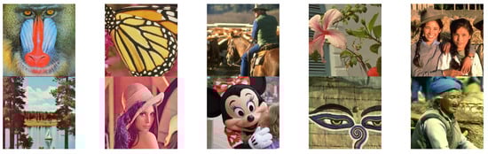
Figure 2.
Test images.
4.1. Objective Assessment
The proposed model in this paper is compared with 11 state-of-the-art models. These models used for comparison include SALSA [38], BPFA [4], GSR [13], NGS [39], TSLRA [40], JPG-SR [14], GSRC-NLP [27], MAR-LOW [41], HSSE [42], IR-CNN [17], and IDBP [43]. Among the comparison models, GSR [13], JPG-SR [14], GSRC-NLP [27], and HSSE [42] are based on traditional GSR or improved GSR models, which are the same type as the proposed multi-color-channels-based GSR model in this paper. In order to comprehensively evaluate the performance of the proposed model for image restoration, the proposed model is also compared with non-GSR-based image restoration models. The BPFA [4] model uses the nonparametric Bayesian dictionary learning method for image sparse representation. The SALSA [38] model proposes an algorithm belonging to the extended Lagrangian method family to deal with constrained problems. The NGS [39] model proposes a new gradient regularization framework using nonlocal similarity. The TSLRA [40] and MAR-LOW [41] are the type of low rank minimization methods. The MAR-LOW [41] combines spatial autoregression with low rank minimization methods and achieves excellent results. The IR-CNN [17] and IDBP [43] are deep-learning-based methods.
Table 1 and Table 2 show the PSNR values of the restoration results on different images under the four pixels missing rates of 80%, 70%, 60% and 50% of the proposed model and the comparison models. In the tables, the best results are highlighted in bold. Table 3 shows the SSIM values of the results on different images under the four pixel missing rates of the proposed model and the comparison models, and the best results are highlighted in bold. Table 1 and Table 2 show the comparison results between the proposed model and the traditional models, and Table 3 shows the comparison results between the proposed model and the deep-learning-based models. In order to reduce the burden of experiments, the result data of NGS [39], TSLRA [40], and HSSE [42], provided in HSSE [42], are used here directly to avoid repetitive implementations. The experimental data of the deep learning methods IR-CNN [17] and IDBP [43] are directly from JPG-SR [14] and GSRC-NLP [27].

Table 1.
PSNR values of the proposed method and some state-of-the-art methods with pixel missing rates 80% and 70%.
Table 2.
PSNR values of the proposed method and some state-of-the-art methods with pixel missing rates 60% and 50%.
Table 3.
PSNR and SSIM values of the proposed method and two deep-learning-based methods with four different pixel missing rates.
In addition to PSNR and SSIM values of each test image, the average PSNR and SSIM values of all test images under different pixel missing rates corresponding to different models are calculated for overall comparison. It can be seen from Table 1, Table 2 and Table 3 that the proposed multi-color-channels-based GSR model in this paper obtains better results than other competitive models. Firstly, the proposed model is compared with the non-GSR-based image restoration models. In terms of the average metric values, the proposed model is 7.20 dB higher than the SALSA model, 7.77 dB higher than the BPFA model, 6.00 dB higher than the NGS model, 4.94 dB higher than the TSLRA model, and 0.06 dB higher than the MAR-LOW model. Among the GSR based models, the JPG-SR method combines the PSR model with the GSR model, and it not only preserves the advantages of the two models, but also reduces their disadvantages, and therefore the sparse representation model is unified. The GSRC-NLP method introduces group sparse residual constraints to the traditional GSR model to approximate the group sparsity of the original group and improve the quality of image restoration. The HSSR model combines the external GSR model with the internal GSR model using the NSS prior knowledge of degraded images and external data sets to optimize the image. However, the above three GSR-based-models and many other improved models not compared in this paper transform the color image into YCbCr space, and only extract the Y channel for processing. In this way, image processing cannot be loyal to each color channel of the original color image, which makes the effect of image restoration poor. The proposed method utilizes three color channels in image restoration to obtain better results, and Table 1 and Table 2 prove this conclusion. Compared with the aforementioned three GSR-based models in terms of average PSNR metric values, the proposed model is 4.15 dB higher than the traditional GSR model, 3.99 dB higher than the JPG-SR model, 3.77 dB higher than the GSRC-NLP model, and 3.70 dB higher than the HSSE model. It can be concluded from Table 1 and Table 2 that the PSNR of the proposed model in this paper on the images with 80%, 70%, 60%, and 50% pixel missing rates are higher than the nine state-of-the-art comparison methods.
Table 3 provides the comparison results of the proposed model with deep-learning-based IR-CNN and ISBP models. In terms of average metric values, the PSNR and SSIM values of the proposed model are 4.1 dB and 0.049 higher than those of the IR-CNN model, and 4.72 dB and 0.067 higher than those of the IDBP model, respectively. It can be seen from the PSNR and SSIM values in Table 3 that the proposed model based on multi-color channels is better than the IR-CNN and IDBP models. The experimental results in Table 1, Table 2 and Table 3 show that the model proposed in this paper is effective and can obtain good restoration results compared with the state-of-the-art models.
4.2. Subjective Assessment
In order to further demonstrate the effectiveness of the proposed multi-color-channels-based GSR model, Figure 3 and Figure 4 respectively show the visual butterfly and girl restoration results of the proposed model and some state-of-the-art models with an 80% pixel missing rate. As can be seen from Figure 3 and Figure 4, the SALSA model cannot restore sharp edges and fine details. The BPFA model can have better visual effects than the salsa model, but it still has undesirable visual artifacts, such as ringing artifacts in Figure 4d. The GSR, JPG-SR and GSRC-NLP models produce over-smoothing effects. Compared with the model proposed in this paper, the MAR-LOW has a similar visual effect, which is not easy to distinguish with the naked eye. However, according to the experimental results in Table 1, Table 2 and Table 3, the proposed model has better objective evaluation results. In general, the visual effects of Figure 3 and Figure 4 show that the GSR model based on multi-color channels proposed in this paper performs best in image restoration. It not only preserves fine details, but also effectively removes visual artifacts.
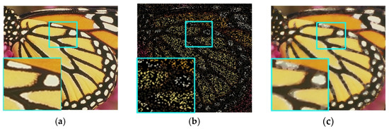
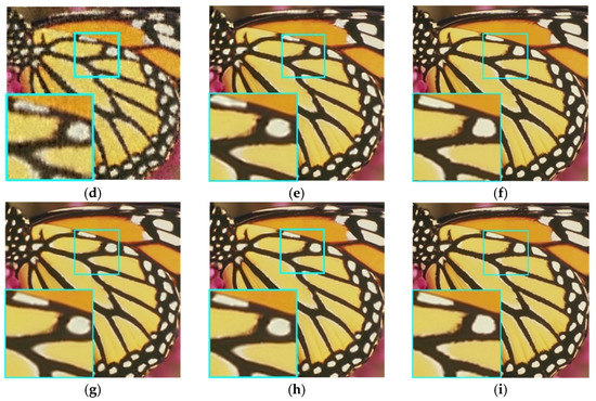
Figure 3.
The restoration results of butterfly with pixel missing rate of 80%. (a) Butterfly, (b) butterfly with pixels missing rate 80%, (c) SALSA [38] (PSNR = 22.85), (d) BPFA [4] (PSNR = 21.06), (e) GSR [13] (PSNR = 26.03), (f) MAR-LOW [41] (PSNR = 30.86), (g) JPG-SR [14] (PSNR = 26.58), (h) GSRC-NLP [27] (PSNR = 26.78), (i) our model (PSNR = 30.90).
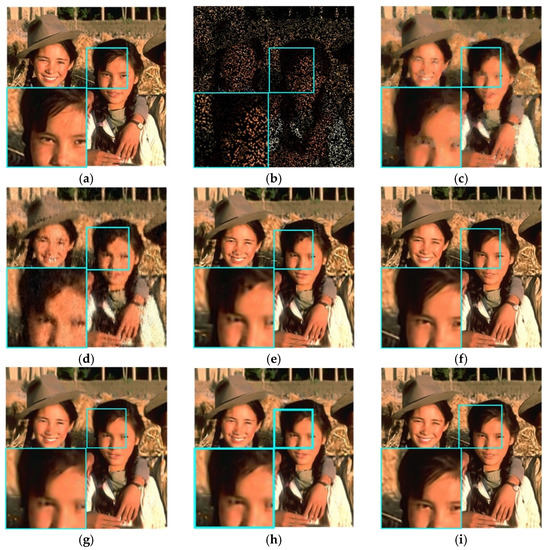
Figure 4.
The restoration result of girl with pixel missing rate of 80%. (a) Girl, (b) girl with pixels missing rate 80%, (c) SALSA [38] (PSNR = 23.79), (d) BPFA [4] (PSNR = 22.47), (e) GSR [13] (PSNR = 25.50), (f) MAR-LOW [41] (PSNR = 29.21), (g) JPG-SR [14] (PSNR = 25.55), (h) GSRC-NLP [27] (PSNR = 26.02), (i) our model (PSNR = 29.28).
5. Conclusions
In order to improve the performance of the traditional GSR model in image restoration, the paper extends the GSR model to a new multi-color-channels-based case, and process R, G, and B color channels of an image simultaneously. The problem of image restoration is transformed into how to use multi-color channels for sparse representation. The alternating minimization method with an adaptive parameter setting strategy is used to solve the proposed multi-color-channels-based model. The proposed method is compared with state-of-the-art methods. The experimental results show that the proposed model can obtain good results in terms of visual effects and quantitative metrics.
Author Contributions
Conceptualization, Y.K., C.Z. (Caiyue Zhou) and C.Z. (Chongbo Zhou); methodology, C.Z. (Chongbo Zhou); software, C.Z. (Caiyue Zhou); validation, Y.K. and C.Z. (Chongbo Zhou); formal analysis, L.S.; investigation, C.Z. (Chuanyong Zhang) and C.Z. (Chongbo Zhou); resources, C.Z. (Chongbo Zhou); data curation, L.S.; writing—original draft preparation, C.Z. (Caiyue Zhou); writing—review and editing, C.Z. (Chongbo Zhou); visualization, L.S.; supervision, C.Z. (Chongbo Zhou); project administration, C.Z. (Chongbo Zhou); funding acquisition, L.S. All authors have read and agreed to the published version of the manuscript.
Funding
The research of this paper was Funded by Ship Control Engineering and Intelligent Systems Engineering Technology Research Center of Shandong Province (Grant Number: SSCC20220003).
Institutional Review Board Statement
Not applicable.
Informed Consent Statement
Not applicable.
Data Availability Statement
Not applicable.
Conflicts of Interest
The authors declare no conflict of interest.
References
- Buades, A.; Coll, B.; Morel, J.M. A Non-Local Algorithm for Image Denoising. In Proceedings of the 2005 IEEE Computer Society Conference on Computer Vision and Pattern Recognition (CVPR’05), San Diego, CA, USA, 20–25 June 2005; pp. 60–65. [Google Scholar]
- Dabov, K.; Foi, A.; Egiazarian, K. Video Denoising by Sparse 3D Transform-Domain Collaborative Filtering. In Proceedings of the 2007 15th European Signal Processing Conference, Poznan, Poland, 3–7 September 2007; pp. 145–149. [Google Scholar]
- Pan, J.; Sun, D.; Pfister, H.; Yang, M.H. Blind Image Deblurring Using Dark Channel Prior. In Proceedings of the 2016 IEEE Conference on Computer Vision and Pattern Recognition, Las Vegas, NV, USA, 27–30 June 2016; pp. 1628–1636. [Google Scholar]
- Zhou, M.; Chen, H.; Paisley, J.; Ren, L.; Li, L.; Xing, Z.; Dunson, D.; Sapiro, G.; Carin, L. Nonparametric Bayesian dictionary learning for analysis of noisy and incomplete images. IEEE Trans. Image Process. 2012, 21, 130–144. [Google Scholar] [CrossRef] [PubMed] [Green Version]
- Jin, K.H.; Ye, J.C. Annihilating filter-based low-rank hankel matrix approach for image inpainting. IEEE Trans. Image Process. A Publ. IEEE Signal Process. Soc. 2015, 24, 3498–3511. [Google Scholar]
- Zhang, J.; Zhao, D.; Zhao, C.; Xiong, R.; Ma, S.; Gao, W. Compressed Sensing Recovery via Collaborative Sparsity. In Proceedings of the 2012 Data Compression Conference, Snowbird, UT, USA, 10–12 April 2012; pp. 287–296. [Google Scholar]
- Yuan, X.; Huang, G.; Jiang, H.; Wilford, P.A. Block-Wise Lensless Compressive Camera. In Proceedings of the 2017 IEEE International Conference on Image Processing, Beijing, China, 17–20 September 2017; pp. 31–35. [Google Scholar]
- Osher, S.; Burger, M.; Goldfarb, D.; Xu, J.; Yin, W. An iterative regularization method for total variation-based image restoration. Siam J. Multiscale Model. Simul. 2005, 4, 460–489. [Google Scholar] [CrossRef]
- Yuan, X. Generalized Alternating Projection Based Total Variation Minimization for Compressive Sensing. In Proceedings of the IEEE International Conference on Image Processing, Phoenix, AZ, USA, 25–28 September 2016; pp. 2539–2543. [Google Scholar]
- Rudin, L. Nonlinear total variation based noise removal algorithms. Phys. D Nonlinear Phenom. 1992, 60, 259–268. [Google Scholar] [CrossRef]
- Li, H.; Liu, F. Image Denoising via Sparse and Redundant Representations over Learned Dictionaries in Wavelet Domain. In Proceedings of the 2009 Fifth International Conference on Image and Graphics, Xi’an, China, 20–23 September 2009; pp. 754–758. [Google Scholar]
- Mairal, J.; Bach, F.; Ponce, J.; Sapiro, G.; Zisserman, A. Non-Local Sparse Models for Image Restoration. In Proceedings of the 2009 IEEE 12th International Conference on Computer Vision, Kyoto, Japan, 29 September–2 October 2009; pp. 2272–2279. [Google Scholar]
- Zhang, J.; Zhao, D.; Gao, W. Group-based sparse representation for image restoration. IEEE Trans. Image Process. A Publ. IEEE Signal Process. Soc. 2014, 23, 3336. [Google Scholar] [CrossRef] [PubMed] [Green Version]
- Zha, Z.; Yuan, X.; Wen, B.; Zhang, J.; Zhou, J.; Zhu, C. Image Restoration Using Joint Patch-Group Based Sparse Representation. IEEE Trans. Image Process. 2020, 29, 7735–7750. [Google Scholar] [CrossRef]
- Liu, Y.; Yuan, X.; Suo, J.; Brady, D.J.; Dai, Q. Rank Minimization for Snapshot Compressive Imaging. IEEE Trans. Pattern Anal. Mach. Intell. 2019, 41, 2990–3006. [Google Scholar] [CrossRef] [Green Version]
- Zhang, J.; Ghanem, B. ISTA-Net: Interpretable Optimization-Inspired Deep Network for Image Compressive Sensing. In Proceedings of the 2018 IEEE/CVF Conference on Computer Vision and Pattern Recognition, Salt Lake City, UT, USA, 18–23 June 2018; pp. 1828–1837. [Google Scholar]
- Zhang, K.; Zuo, W.; Gu, S.; Zhang, L. Learning Deep CNN Denoiser Prior for Image Restoration. In Proceedings of the 2017 IEEE Conference on Computer Vision and Pattern Recognition, Honolulu, HI, USA, 21–26 July 2017; pp. 2808–2817. [Google Scholar]
- Dong, W.; Wang, P.; Yin, W.; Shi, G.; Wu, F.; Lu, X. Denoising prior driven deep neural network for image restoration. IEEE Trans. Pattern Anal. Mach. Intell. 2019, 41, 2305–2318. [Google Scholar] [CrossRef] [Green Version]
- Yang, J.; Wright, J.; Huang, T.S.; Ma, Y. Image super-resolution via sparse representation. IEEE Trans. Image Process. 2010, 19, 2861–2873. [Google Scholar] [CrossRef]
- Aharon, M.; Elad, M.; Bruckstein, A. K-SVD: An algorithm for designing overcomplete dictionaries for sparse representation. IEEE Trans. Signal Process. 2006, 54, 4311–4322. [Google Scholar] [CrossRef]
- Lun, D.P.K. Robust fringe projection profilometry via sparse representation. IEEE Trans. Image Process. 2016, 25, 1726–1739. [Google Scholar]
- Dong, W.; Zhang, L.; Shi, G.; Wu, X. Image deblurring and super-resolution by adaptive sparse domain selection and adaptive regularization. IEEE Trans. Image Process. 2011, 20, 1838–1857. [Google Scholar] [CrossRef] [PubMed] [Green Version]
- Wang, Q.; Zhang, X.; Wu, Y.; Tang, L.; Zha, Z. Nonconvex weighted lp minimization based group sparse representation framework for image denoising. IEEE Signal Process. Lett. 2017, 24, 1686–1690. [Google Scholar] [CrossRef]
- Dong, W.; Shi, G.; Li, X. Nonlocal image restoration with bilateral variance estimation: A low-rank approach. IEEE Trans. Image Process. A Publ. IEEE Signal Process. Soc. 2013, 22, 700–711. [Google Scholar] [CrossRef] [PubMed]
- Dong, W.; Shi, G.; Ma, Y.; Li, X. Image restoration via simultaneous sparse coding: Where structured sparsity meets gaussian scale mixture. Int. J. Comput. Vis. 2015, 114, 217–232. [Google Scholar] [CrossRef]
- Zha, Z.; Yuan, X.; Wen, B.; Zhou, J.; Zhang, J.; Zhu, C. A Benchmark for Sparse Coding: When Group Sparsity Meets Rank Minimization. IEEE Trans. Image Process. 2020, 29, 5094–5109. [Google Scholar] [CrossRef] [Green Version]
- Zha, Z.; Yuan, X.; Wen, B.; Zhou, J.; Zhu, C. Group sparsity residual constraint with non-local priors for image restoration. IEEE Trans. Image Process. 2020, 29, 8960–8975. [Google Scholar] [CrossRef]
- Xu, J.; Zhang, L.; Zuo, W.; Zhang, D.; Feng, X. Patch Group Based Nonlocal Self-Similarity Prior Learning for Image Denoising. In Proceedings of the 2015 IEEE International Conference on Computer Vision, Santiago, Chile, 7–13 December 2015; pp. 244–252. [Google Scholar]
- Zha, Z.; Liu, X.; Huang, X.; Shi, H.; Xu, Y.; Wang, Q.; Tang, L.; Zhang, X. Analyzing the Group Sparsity Based on the Rank Minimization Methods. In Proceedings of the 2017 IEEE International Conference on Multimedia and Expo, Hong Kong, China, 10–14 July 2017; pp. 883–888. [Google Scholar]
- Hu, W.; Li, X.; Cheung, G.; Au, O. Depth Map Denoising Using Graph-Based Transform and Group Sparsity. In Proceedings of the 2013 IEEE 15th International Workshop on Multimedia Signal Processing, Pula, Italy, 30 September–2 October 2013; pp. 1–6. [Google Scholar]
- Routray, S.; Ray, A.K.; Mishra, C. An efficient image denoising method based on principal component analysis with learned patch groups. Signal Image Video Process. 2019, 13, 1405–1412. [Google Scholar] [CrossRef]
- Mo, J.; Zhou, Y. The research of image inpainting algorithm using self-adaptive group structure and sparse representation. Clust. Comput. 2018, 22, 7593–7601. [Google Scholar] [CrossRef]
- Wen, B.; Ravishankar, S.; Bresler, Y. Structured overcomplete sparsifying transform learning with convergence guarantees and applications. Int. J. Comput. Vis. 2015, 114, 137–167. [Google Scholar] [CrossRef]
- Elad, M.; Yavneh, I. A plurality of sparse representations is better than the sparsest one alone. IEEE Trans. Inf. Theory 2009, 55, 4701–4714. [Google Scholar] [CrossRef]
- Daubechies, I.; Defrise, M.; Mol, C.D. An iterative thresholding algorithm for linear inverse problems with a sparsity constraint. Commun. Pure Appl. Math. 2010, 57, 1413–1457. [Google Scholar] [CrossRef] [Green Version]
- Chang, S.G.; Yu, B. Adaptive wavelet thresholding for image denoising and compression. IEEE Trans. Image Process. A Publ. IEEE Signal Process. Soc. 2000, 9, 1532. [Google Scholar] [CrossRef] [PubMed] [Green Version]
- Wang, Z.; Bovik, A.C.; Sheikh, H.R.; Simoncelli, E.P. Image quality assessment: From error visibility to structural similarity. IEEE Trans. Image Process. 2004, 13, 600–612. [Google Scholar] [CrossRef] [PubMed] [Green Version]
- Afonso, M.V.; Bioucas-Dias, J.M.; Figueiredo, M.A. An augmented Lagrangian approach to the constrained optimization formulation of imaging inverse problems. IEEE Trans. Image Process. 2011, 20, 681–695. [Google Scholar] [CrossRef] [PubMed] [Green Version]
- Liu, H.; Xiong, R.; Zhang, X.; Zhang, Y.; Ma, S.; Gao, W. Nonlocal gradient sparsity regularization for image restoration. IEEE Trans. Circuits Syst. Video Technol. 2017, 27, 1909–1921. [Google Scholar] [CrossRef]
- Guo, Q.; Gao, S.; Zhang, X.; Yin, Y.; Zhang, C. Patch-based image inpainting via two-stage low rank approximation. IEEE Trans. Vis. Comput. Graph. 2017, 24, 2023–2036. [Google Scholar] [CrossRef]
- Li, M.; Liu, J.; Xiong, Z.; Sun, X.; Guo, Z. MARLow: A Joint Multiplanar Autoregressive and Low-Rank Approach for Image Completion. In Proceedings of the European Conference on Computer Vision, Amsterdam, The Netherlands, 8–16 October 2016; pp. 819–834. [Google Scholar]
- Zha, Z.; Wen, B.; Yuan, X.; Zhou, J.; Zhu, C.; Kot, A.C. A hybrid structural sparsification error model for image restoration. IEEE Trans. Neural Netw. Learn. Syst. 2021. [Google Scholar] [CrossRef]
- Tirer, T.; Giryes, R. Image restoration by iterative denoising and backward projections. IEEE Trans. Image Process. 2019, 28, 1220–1234. [Google Scholar] [CrossRef]
Publisher’s Note: MDPI stays neutral with regard to jurisdictional claims in published maps and institutional affiliations. |
© 2022 by the authors. Licensee MDPI, Basel, Switzerland. This article is an open access article distributed under the terms and conditions of the Creative Commons Attribution (CC BY) license (https://creativecommons.org/licenses/by/4.0/).