Abstract
The human immunodeficiency virus (HIV) mainly attacks CD4+ T cells in the host. Chronic HIV infection gradually depletes the CD4+ T cell pool, compromising the host’s immunological reaction to invasive infections and ultimately leading to acquired immunodeficiency syndrome (AIDS). The goal of this study is not to provide a qualitative description of the rich dynamic characteristics of the HIV infection model of CD4+ T cells, but to produce accurate analytical solutions to the model using the modified iterative approach. In this research, a new efficient method using the new iterative method (NIM), the coupling of the standard NIM and Laplace transform, called the modified new iterative method (MNIM), has been introduced to resolve the HIV infection model as a class of system of ordinary differential equations (ODEs). A nonlinear HIV infection dynamics model is adopted as an instance to elucidate the identification process and the solution process of MNIM, only two iterations lead to ideal results. In addition, the model has also been solved using NIM and the fourth order Runge–Kutta (RK4) method. The results indicate that the solutions by MNIM match with those of RK4 method to a minimum of eight decimal places, whereas NIM solutions are not accurate enough. Numerical comparisons between the MNIM, NIM, the classical RK4 and other methods reveal that the modified technique has potential as a tool for the nonlinear systems of ODEs.
1. Introduction
Differential equations are the foundation of many scientific and engineering problems [1]. Differential equations are equations that express a relationship between certain variables and their derivatives. Variables are changing entities in mathematics, and the rate of change of one variable with respect to another is called a derivative [2].
In addition, an ordinary differential equation (ODE) is an equation that involves some ordinary derivatives of a function. In general, physical systems in nature consist of complicated phenomena for which accurate solutions can be difficult to compute. Numerical or semi-analytical methods may be preferable in such instances. In this context, there are numerous standard books [3,4,5,6,7] on the solution of ordinary differential equations (ODEs). A first attempt at classifying ODE systems is with respect to the initial or boundary conditions connected with them, both mathematically and computationally [8]. It should be mentioned that the numerical solution of ordinary differential equations is a very active and ongoing topic of research [9].
Infectious diseases frequently affect a huge number of people spread across vast geographical regions. Mathematical models of ordinary differential equations have significance in studying the dynamic behavior of infectious diseases. In recent times, many mathematical models including mumps virus [10], ebola virus disease [11], dengue fever disease [12], rubella disease [13], influenza transmission [14], zika virus transmission [15], COVID-19 pandemic [16,17,18] and many others have been formulated using differential equations.
In the present study, the HIV infection model of CD4+ T cells has been investigated mathematically. HIV infection targets CD4+ T cells, the immune system’s biggest white blood cells. HIV infection has a severe devastating impact on CD4+ T cells, killing them and weakening the immune system. When the number of CD4+ T cells falls below a particular threshold, the cell-mediated immune system vanishes, the immune system weakens, and the body is more likely to be infected [19]. The HIV infection model is represented by the standard three-compartmental system [20], such as susceptible CD4+ T cell concentration, CD4+ T cell infection and free HIV viral substance in the blood. They are denoted by time dependent variables such as and . A system of nonlinear differential equations characterizes this model are as follows:
Let us assume the initial conditions are as follows:
Several typical approaches to numerically address the HIV infection of the CD4+ T cells model have recently been introduced in the literature. For instance, Ongun [21] used the Laplace–Adomian decomposition method (LADM) to solve the HIV infection model. Merdan et al. [22] had developed the multi-stage variational iteration approach (MSVIM). In order to solve the HIV infection model, Yüzbaş [23] introduced the Bessel collocation approach. Doğan [24] solved the model using the multi-step Laplace–Adomian decomposition method (MSLADM). Merdan [25] employed the homotopy perturbation method (HPM) on the determined system. Merdan et al. [26] recently used the modified variational iteration technique (MVIM) to get the approximate solutions of (1)–(3). Goreishi et al. [27] used the homotopy analysis method (HAM) to resolve the variation of the noted model. To acquire the numeric solution of the HIV model, the stochastic global search approach known as genetic algorithm (GA) is combined with two local search optimizers known as interior point algorithm (IPA) and active set algorithm (ASA) in [28]. Very recently, Attaullah and Sohaib [29] used continuous Galerkin–Petrov (cGP) and the Legendre wavelet collocation method (LWCM) for the approximate solution to the selected mathematical model.
For the general nonlinear problem, the new iterative method (NIM) has received a lot of attention since it requires no multiplier or polynomials for nonlinear terms of the problems. The NIM algorithm was developed by Daftardar-Gejji and Jafari [30] to solve stochastic and deterministic problems. Recently, Adwan et al. [31] used NIM to identify analytical and numerical solutions for linear and nonlinear multidimensional problems. The approximate solutions for second order nonlinear ordinary differential equations (ODEs) have been provided by Al-Jawary et al. [32] using NIM. By using semi analytic NIM, the nonlinear problem of Jeffery–Hamel flow has been solved analytically and numerically by AL-Jawary et al. [33]. Alderremy et al. [34] have extended the applications of NIM to find the solutions of Klein–Gordon equations (KGEs), which have been applied in the modeling of spin wave, quantum field theory, kink dynamics, astrophysics, cosmology and classical mechanics. First, they reduced the level of calculation by using the Elzaki transform method and then solved the corresponding equations with the help of NIM. Recently, the technique has been applied widely to several dynamical systems (see [35,36,37,38,39]).
The design of semi-analytical methods such as the Adomian decomposition, homotopy perturbation, variational iteration approaches and new iterative method (NIM) differ from each other. Although these methods provide some helpful solutions that are frequently represented in terms of polynomials and the region of convergences (ROCs) is relatively small in certain nonlinear problems such as the HIV infection model. Both perturbation techniques and non-perturbative approaches cannot provide a straightforward procedure for adjusting or controlling the convergence region and rate of a given approximation series [27]. So it is occasionally essential to improve them. Also, the recent results provided in the literature of Attaullah and Sohaib [21], used continuous Galerkin–Petrov (cGP) and the Legendre wavelet collocation method (LWCM) to match at least four decimal places with RK4, which is considered to be more accurate than all previous results published, so there could be the scope for further investigation to attain more accuracy.
The goal of this research is to modify the new iterative method (NIM) by implementing the modified new iterative method (MNIM), i.e., the combination of Laplace transformation and NIM to solve the class of nonlinear HIV infection model and achieve higher accuracy than previous methods.
The rest of the present study is presented as: the solution procedure of NIM and modified NIM are interpreted in Section 2. The applications of both NIM and MNIM for the considered HIV infection model are introduced in Section 3. The results and discussion of the present methods are illustrated in Section 4, and then the concluding remarks of the research has been given in Section 5.
2. Solution Procedure
2.1. Basic Idea of NIM
In this section we have discussed the new iterative method (NIM) as follows. Consider a general equation:
where is a linear operator and is a nonlinear operator from a Banach space and is a given analytic function. The solution for Equation (5) having in the series form,
Since is linear,
The nonlinear operator can be decomposed as follows:
Thus, according to NIM,
Therefore,
Therefore, we define the recursive relation:
Then series solution becomes
Therefore,
2.2. The Modified New Iterative Method (MNIM)
In this section we have proposed a modification of NIM using the combination of Laplace transform with the new iterative method to solve system of differential equations. Let us consider a system of differential equations in the operator form:
subjected to the initial conditions
where is an invertible linear differential operator, and are remaining linear operators order less than and are nonlinear operators and are inhomogeneous terms. For the first order , second order and so on.
The technique consists first of applying Laplace transformation (which is denoted by ℑ) to both sides of systems (22)–(24), hence,
Applying the formulas for Laplace transforms, we obtain
where ‘’ is called a Laplace domain function.
Using the initial conditions (25), we have,
applying the inverse Laplace transform to the equations in (32)–(34), we get
Let the approximate solutions of system be expressed as
For the NIM, the nonlinear operators can be decomposed by,
Since are linear,
The NIM admits the use of the recursive relations in the following way:
where is the term arising after inverse Laplace transformation of the source term all of which are assumed to be prescribed.
Thus,
By a similar manner, we have
and
2.3. Convergence Analysis of MNIM
Let, be the elements in a Banach space , and is nonlinear contraction from such that . Then according to the principle of Banach fixed-point theorem, converges if .
Proof.
In general, let us take
where is the initial approximation, is a known function in Banach space , is an arbitrary constant and . We can write
Hence, the series , (where and ) absolutely and uniformly converges, which is unique in view of the Banach contraction principle. □
3. Application
3.1. NIM for HIV Infection Model
Here we introduce numerical outline of NIM for the approximate solution of the HIV infection model. Let the integration on the system (1)–(3), using initial conditions (4) and parameters of Table 1.

Table 1.
List of parameters used in the HIV infection model.
In view of (14)–(18) and according to the solution procedure of NIM for system of differential equations, we find the approximations as follows:
The next successive iterations can be obtained in a similar manner.
Therefore,
For the computation purpose we have taken the 5-iterations of NIM solutions.
3.2. MNIM for the HIV Infection Model
Let us first apply the Laplace transform on both sides of Equations (1)–(3) and using the initial conditions (4) and model parameters discussed in Table 1.
Again, applying the inverse Laplace transform on both sides of Equations (76)–(78), we get
In view of (47)–(58), solutions are obtained by using MNIM, as follows
The next successive iterations can be obtained in a similar manner.
Therefore,
For the computation purpose we have taken the 2-iterations of MNIM solutions.
4. Results and Discussions
We take a scenario of Attaullah et al. [29], where the initial conditions are , with parameter values . All our calculations as well as our graphs are carried out by Maple 2020. The Maple built-in programme has been used for RK4 solutions with step size . The new iterative method (NIM) and modified new iterative method’s (MNIM) simulation results are illustrated graphically and numerically. We displayed the graphical outcomes of both NIM and MNIM strategies related to the RK4 method in Figure 1. The figure depicts that the 5-iterations of NIM solutions fail to provide suitable accuracy as time increases and solutions are only valid till , whereas the 2-iterations of modified NIM precisions agree well with those of RK4 precisions. Additionally, we contrasted the absolute errors of the proposed MNIM scheme to those of other conventional methods, such as cGP(2) and LWCM [29], GA-IPA and GA-ASA [28], LADM-Padé [21], MVIM [26], HPM [25], Bessel collocation [23] and NIM relative to RK4 method, as shown in Table 2, Table 3 and Table 4 for , respectively. The recent results via cGP(2) and LWCM [29] match to at least four decimal places with RK4. Further, the numeric solutions via NIM matched at least one decimal place with RK4. In contrast, the results show that the solutions by 2-iterations of MNIM match with those of RK4 at least eight decimal places. The comparisons with other methods used for the model clearly indicate that the MNIM scheme outperformed all the pre-existing solutions. Therefore, it suggests the high accuracy and validity of the proposed MNIM scheme with fewer iterative steps.
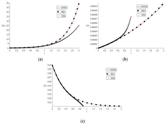
Figure 1.
Graphical Comparison between the results of 2-Iterations MNIM, 5-Iterations NIM and RK4 method for (a) , (b) , (c) of HIV Infection Model.
Table 2.
Comparison of Absolute Errors for of MNIM Scheme and LWCM, cGP(2), GA-IPA, GA-ASA, LADM-Padé, MVIM, HPM, Bessel collocation, NIM relative to RK4 Method for HIV Infection Model.
Table 3.
Comparison of Absolute Errors for of MNIM Scheme and LWCM, cGP(2), GA-IPA, GA-ASA, LADM-Padé, MVIM, HPM, Bessel collocation, NIM relative to RK4 Method for HIV Infection Model.
Table 4.
Comparison of Absolute Errors for of MNIM Scheme and LWCM, cGP(2), GA-IPA, GA-ASA, LADM-Padé, MVIM, HPM, Bessel collocation, NIM relative to RK4 Method for HIV Infection Model.
5. Conclusions
In this paper, we propose an improvement to the existing new iterative method and prove that the improved method is more accurate than the new iterative method for solving a system of nonlinear differential equations that describes HIV infection in CD4+ T cells. The MNIM helps us to reduce the number of terms as well as iterations steps. The modified NIM solutions are more accurate than other numeric solutions of the HIV infection model. The recent results provided in Ref. [29], matches to at least four decimal places with RK4, in contrast, MNIM matches to at least eight decimal places. Furthermore, based on our observations, the numerical solutions of 5-iterations of NIM for the HIV infection model were valid only in a short time span () and the modified NIM is used to extend the validity domains for selected disease model, calculating only 2-iteration steps. The modified method provides the solution in a rapid convergent series with computable terms. Analytic-numeric solutions were used to ensure that the MNIM technique is straightforward, reliable, and efficient. We hope that the modified iterative algorithm will be able to solve many types of interesting nonlinear problems. The implementation of this method in HIV infection dynamics may pave the way for a new horizon in the future. Future work should reapply these methods in developing a dynamic model for other diseases such as heart disease [40,41,42] and combine the proposed approach with the machine learning model to develop optimal solutions for infectious diseases such as COVID-19 and pneumonia [43,44,45].
Author Contributions
Conceptualization, I.G., M.M.R., S.M.; methodology, I.G., M.M.R.; validation, M.M.A., K.D.G., M.R.U.; formal analysis, M.M.A., K.D.G., M.R.U.; writing—original draft preparation, I.G., M.M.R., S.M.; writing—review and editing, I.G., M.M.R., S.M., R.R., M.M.A., K.D.G., M.R.U., P.G.; supervision, M.M.R. All authors have read and agreed to the published version of the manuscript.
Funding
This research received no external funding.
Institutional Review Board Statement
Not applicable.
Informed Consent Statement
Not applicable.
Data Availability Statement
Not applicable.
Conflicts of Interest
The authors declare no conflict of interest.
References
- Chakraverty, S.; Mahato, N.R.; Karunakar, P.; Rao, T.D. Advanced Numerical and Semi-Analytical Methods for Differential Equations; John Wiley & Sons, Inc.: Hoboken, NJ, USA, 2019; ISBN 9781119423423. [Google Scholar]
- Tenenbamn, M.; Pollard, H. Ordinary Differential Equations: An Elementary Textbook for Students of Mathematics, Engineering, and the Sciences; Dover publications Inc.: New York, NY, USA, 1963; ISBN 0486649407. [Google Scholar]
- Alexander, R. Solving Ordinary Differential Equations I: Nonstiff Problems (E. Hairer, SP Norsett, and G. Wanner). Siam Rev. 1990, 32, 485. [Google Scholar] [CrossRef]
- Hall, G.; Watt, J.M.; Hall, G.; Watt, J.W.; Watt, M. Modern Numerical Methods for Ordinary Differential Equations; Oxford University Press: Oxford, UK, 1976; ISBN 0198533489. [Google Scholar]
- Stetter, H.J. Analysis of Discretization Methods for Ordinary Differential Equations; Springer: Berlin/Heidelberg, Germany, 1973; Volume 23, ISBN 0387060081. [Google Scholar]
- Ortega, J.M.; Poole, W.G. An Introduction to Numerical Methods for Differential Equations; Pitman Publishing: London, UK, 1981; ISBN 0273016377. [Google Scholar]
- Polyanin, A.D.; Zaitsev, V.F. Handbook of Ordinary Differential Equations; Chapman and Hall/CRC: London, UK, 2017; ISBN 9781466569379. [Google Scholar]
- Ascher, U.M.; Petzold, L.R. Computer Methods for Ordinary Differential Equations and Differential-Algebraic Equations; SIAM: Philadelphia, PA, USA, 1997. [Google Scholar]
- Epperson, J.F. An Introduction to Numerical Methods and Analysis; John Wiley & Sons, Inc.: Hoboken, NJ, USA, 2013; ISBN 9781118367599. [Google Scholar]
- Mohammadi, H.; Kumar, S.; Rezapour, S.; Etemad, S. A Theoretical Study of the Caputo–Fabrizio Fractional Modeling for Hearing Loss Due to Mumps Virus with Optimal Control. Chaos Solitons Fractals 2021, 144, 110668. [Google Scholar] [CrossRef]
- Zhang, Z.; Jain, S. Mathematical Model of Ebola and Covid-19 with Fractional Differential Operators: Non-Markovian Process and Class for Virus Pathogen in the Environment. Chaos Solitons Fractals 2020, 140, 110175. [Google Scholar] [CrossRef] [PubMed]
- Shah, K.; Jarad, F.; Abdeljawad, T. On a Nonlinear Fractional Order Model of Dengue Fever Disease under Caputo-Fabrizio Derivative. Alexandria Eng. J. 2020, 59, 2305–2313. [Google Scholar] [CrossRef]
- Baleanu, D.; Mohammadi, H.; Rezapour, S. A Mathematical Theoretical Study of a Particular System of Caputo–Fabrizio Fractional Differential Equations for the Rubella Disease Model. Adv. Differ. Equ. 2020, 2020, 184. [Google Scholar] [CrossRef]
- Rezapour, S.; Mohammadi, H. A Study on the AH1N1/09 Influenza Transmission Model with the Fractional Caputo–Fabrizio Derivative. Adv. Differ. Equ. 2020, 2020, 488. [Google Scholar] [CrossRef]
- Rezapour, S.; Mohammadi, H.; Jajarmi, A. A New Mathematical Model for Zika Virus Transmission. Adv. Differ. Equ. 2020, 2020, 589. [Google Scholar] [CrossRef]
- Batistela, C.M.; Correa, D.P.F.; Bueno, Á.M.; Piqueira, J.R.C. SIRSi Compartmental Model for COVID-19 Pandemic with Immunity Loss. Chaos Solitons Fractals 2020, 2020, 110388. [Google Scholar] [CrossRef]
- Basnarkov, L. SEAIR Epidemic Spreading Model of COVID-19. Chaos Solitons Fractals 2021, 142, 110394. [Google Scholar] [CrossRef]
- Panwar, V.S.; Sheik Uduman, P.S.; Gómez-Aguilar, J.F. Mathematical Modeling of Coronavirus Disease COVID-19 Dynamics Using CF and ABC Non-Singular Fractional Derivatives. Chaos Solitons Fractals 2021, 2021, 110757. [Google Scholar] [CrossRef]
- Baleanu, D.; Mohammadi, H.; Rezapour, S. Analysis of the Model of HIV-1 Infection of CD4+ T-Cell with a New Approach of Fractional Derivative. Adv. Differ. Equ. 2020, 2020, 71. [Google Scholar] [CrossRef] [Green Version]
- Wang, L.; Li, M.Y. Mathematical Analysis of the Global Dynamics of a Model for HIV Infection of CD4+ T Cells. Math. Biosci. 2006, 200, 44–57. [Google Scholar] [CrossRef] [PubMed]
- Ongun, M.Y. The Laplace Adomian Decomposition Method for Solving a Model for HIV Infection of CD4+T Cells. Math. Comput. Model. 2011, 53, 597–603. [Google Scholar] [CrossRef]
- Merdan, M.; Gokdogan, A.; Erturk, V.S. An Approximate Solution of a Model for HIV Infection of CD4+ T Cells. Iran. J. Sci. Technol. Trans. A Sci. 2011, 35, 9–12. [Google Scholar]
- Yüzbaşi, Ş. A Numerical Approach to Solve the Model for HIV Infection of CD4+ T Cells. Appl. Math. Model. 2012, 36, 5876–5890. [Google Scholar] [CrossRef]
- Doǧan, N. Numerical Treatment of the Model for HIV Infection of CD4+ T Cells by Using Multistep Laplace Adomian Decomposition Method. Discret. Dyn. Nat. Soc. 2012, 2012, 976352. [Google Scholar] [CrossRef] [Green Version]
- Merdan, M. Homotopy Perturbation Method for Solving a Model for HIV Infection of CD4+ T Cells. İstanbul Ticaret Üniv. Fen Bilim. Derg. 2007, 6, 39–52. [Google Scholar]
- Merdan, M.; Gökdoǧan, A.; Yildirim, A. On the Numerical Solution of the Model for HIV Infection of CD4+ T Cells. Comput. Math. Appl. 2011, 62, 118–123. [Google Scholar] [CrossRef] [Green Version]
- Ghoreishi, M.; Ismail, A.I.B.M.; Alomari, A.K. Application of the Homotopy Analysis Method for Solving a Model for HIV Infection of CD4+ T-Cells. Math. Comput. Model. 2011, 54, 3007–3015. [Google Scholar] [CrossRef]
- Malik, S.A.; Qureshi, I.M.; Amir, M.; Malik, A.N. Nature Inspired Computational Approach to Solve the Model for HIV Infection of CD4+ T Cells. Res. J. Recent Sci. 2014, 3, 67–76. [Google Scholar]
- Attaullah; Sohaib, M. Mathematical Modeling and Numerical Simulation of HIV Infection Model. Results Appl. Math. 2020, 7, 100118. [Google Scholar] [CrossRef]
- Daftardar-Gejji, V.; Jafari, H. An Iterative Method for Solving Nonlinear Functional Equations. J. Math. Anal. Appl. 2006, 316, 753–763. [Google Scholar] [CrossRef] [Green Version]
- Adwan, M.I.; Al-Jawary, M.A.; Tibaut, J.; Ravnik, J. Analytic and Numerical Solutions for Linear and Nonlinear Multidimensional Wave Equations. Arab J. Basic Appl. Sci. 2020, 27, 166–182. [Google Scholar] [CrossRef] [Green Version]
- Al-Jawary, M.A.; Adwan, M.I.; Radhi, G.H. Three Iterative Methods for Solving Second Order Nonlinear ODEs Arising in Physics. J. King Saud Univ.-Sci. 2020, 32, 312–323. [Google Scholar] [CrossRef]
- AL-Jawary, M.A.; Abdul Nabi, A.Z.J. Three Iterative Methods for Solving Jeffery-Hamel Flow Problem. Kuwait J. Sci. 2020, 47, 1–13. [Google Scholar]
- Alderremy, A.A.; Elzaki, T.M.; Chamekh, M. New Transform Iterative Method for Solving Some Klein-Gordon Equations. Results Phys. 2018, 10, 655–659. [Google Scholar] [CrossRef]
- Ghosh, I.; Chowdhury, M.S.H.; Mt Aznam, S.; Rashid, M.M. Measuring the Pollutants in a System of Three Interconnecting Lakes by the Semianalytical Method. J. Appl. Math. 2021, 2021, 6664307. [Google Scholar] [CrossRef]
- Ghosh, I.; Chowdhury, M.S.H.; Mt Aznam, S.; Mawa, S. New Iterative Method for Solving Chemistry Problem. AIP Conf. Proc. 2021, 2365, 020012. [Google Scholar]
- Chowdhury, M.S.H.; Ghosh, I.; Aznam, S.M.; Mawa, S. A Novel Iterative Method for Solving Chemical Kinetics System. J. Low Freq. Noise Vib. Act. Control 2021, 40, 1731–1743. [Google Scholar] [CrossRef]
- Shah, Z.; Nawaz, R.; Kumam, P.; Farid, S. Application of New Iterative Method to Time Fractional Whitham–Broer–Kaup Equations. Front. Phys. 2020, 8, 104. [Google Scholar] [CrossRef]
- Ahsan, M.M.; Siddique, Z. Machine learning-based heart disease diagnosis: A systematic literature review. Artif. Intell. Med. 2022, 122, 102289. [Google Scholar] [CrossRef] [PubMed]
- Ahsan, M.M.; Luna, S.A.; Siddique, Z. Machine-Learning-Based Disease Diagnosis: A Comprehensive Review. Healthcare 2022, 10, 541. [Google Scholar] [CrossRef] [PubMed]
- Ahsan, M.M.; Mahmud, M.A.; Saha, P.K.; Gupta, K.D.; Siddique, Z. Effect of data scaling methods on machine learning algorithms and model performance. Technologies 2021, 9, 52. [Google Scholar] [CrossRef]
- Ahsan, M.M.; Nazim, R.; Siddique, Z.; Huebner, P. Detection of COVID-19 patients from CT scan and chest X-ray data using modified MobileNetV2 and LIME. Healthcare 2021, 9, 1099. [Google Scholar] [CrossRef]
- Ahsan, M.M.; Ahad, M.T.; Soma, F.A.; Paul, S.; Chowdhury, A.; Luna, S.A.; Yazdan, M.M.; Rahman, A.; Siddique, Z.; Huebner, P. Detecting SARS-CoV-2 from chest X-Ray using artificial intelligence. IEEE Access 2021, 9, 35501–35513. [Google Scholar] [CrossRef]
- Ahsan, M.M.; Gupta, K.D.; Islam, M.M.; Sen, S.; Rahman, M.; Shakhawat Hossain, M. COVID-19 symptoms detection based on nasnetmobile with explainable ai using various imaging modalities. Mach. Learn. Knowl. Extr. 2020, 2, 490–504. [Google Scholar] [CrossRef]
- Ahsan, M.M.; EAlam, T.; Trafalis, T.; Huebner, P. Deep MLP-CNN model using mixed-data to distinguish between COVID-19 and Non-COVID-19 patients. Symmetry 2020, 12, 1526. [Google Scholar] [CrossRef]
Publisher’s Note: MDPI stays neutral with regard to jurisdictional claims in published maps and institutional affiliations. |
© 2022 by the authors. Licensee MDPI, Basel, Switzerland. This article is an open access article distributed under the terms and conditions of the Creative Commons Attribution (CC BY) license (https://creativecommons.org/licenses/by/4.0/).