Accelerate Incremental TSP Algorithms on Time Evolving Graphs with Partitioning Methods

Abstract

In time-evolving graphs, the graph changes at each time interval, and the previously computed results become invalid. We addressed this issue for the traveling salesman problem (TSP) in our previous work and proposed an incremental algorithm where the TSP tour is computed from the previous result instead of the whole graph. In our current work, we have mapped the TSP problem to three partitioning methods named vertex size attribute, edge attribute, and k-means; then, we compared the TSP tour results. We have also examined the effect of increasing the number of partitions on the total computation time. Through our experiments, we have observed that the vertex size attribute performs the best because of a balanced number of vertices in each partition.

1. Introduction

A graph is a commonly used data structure used to represent data with relationships. In the real world, graphs are used in the transportation systems, biological networks, social media graphs, and so on. Time-evolving graphs (TEG) are the graphs that evolve with time. Generally, there can be the following update events on a graph: edge/vertex addition, deletion, and changes in weight. These update events change the structure of the TEG. Traditionally, these graphs are computed by building a set of graph snapshots of the data and applying the static graph techniques to them. However, the maintenance of graph snapshots is expensive when the volume and the velocity of update event increase and leads to wastage in terms of memory storage and computation power. Developing an efficient algorithm for TEG is a critical and, at the same time, a challenging task, too.

The traveling salesman problem (TSP) computes the shortest tour originating from a source vertex in a given graph by visiting each vertex exactly once. Solving TSP [1] is time consuming as well as computationally expensive because it is a NP-hard problem [2]. TSP is a commonly seen graph problem that can be applicable to a variety of applications in the field of robotics [3], trajectory planning for electromagnetic docking [4,5,6], and operation research [7]. The TSP problem can be mapped to various real-life applications and leads to an extended version of TSP such as Clustered TSP [8], Generalized TSP [9,10,11], and Multiple TSP [12,13]. Applying those algorithms to TEG leads to significant recomputation overhead whenever a graph change event occurs. Hence, traditional approaches will not be feasible on rapidly evolving graphs.

In our previous work, we have addressed the challenge of TEG by proposing an incremental algorithm [14]. The proposed incremental algorithms (I-TSP and Ig-TSP) minimized the number of recomputations on the graph by only computing the affected part of the graph and maintained the TSP tour across time intervals. We have further reduced the computation time of the I-TSP and Ig-TSP algorithms by defining a partitioning method [15] on top if it. The proposed partitioning algorithms (P-TSP and Pg-TSP) partition the graph in sub-graphs and compute sub-tours independently on each sub-graph. Then, these sub-tours are connected to form a tour through all the partitions. From our experimental results, we observed that the computation time can be significantly reduced for incremental algorithms (I-TSP and Ig-TSP) by using partitioning TSP algorithms (P-TSP and Pg-TSP), and the time reduction can be greater under a higher number of partitions.

In this work, we have mapped our TSP problem to three partitioning methods named (1) Vertex size attribute-based partitioning, (2) Edge size attribute-based partitioning, and (3) k-means clustering-based partitioning. We have compared the result in terms of total computation time taken and the number of messages sent in computation. We have also examined the effect of increasing the number of partitions on the total computation time. Through our experiments, we have observed that the vertex size attribute performs the best because of the balanced number of vertices in each partition. Apart from experiments, we have provided the complexity analysis of the proposed algorithm in terms of number of messages and number of paths.

The rest of the sections are structured as follows: Section 2 describes related works. The problem is defined in Section 3 along with the proposed algorithms. Section 4 discusses the complexity analysis. Section 5 presents the experiment results, and Section 6 concludes the paper.

2. Background and Related Work

This paper focuses on various domains, and hence, the related work is divided into four sub-sections: namely, time-evolving graphs, the traveling salesman problem, incremental algorithm, and graph partitioning. In the end, our paper is compared with some state-of-the-art research works in

Table 1. Comparing state-of-the-art algorithms on the basis of approach used in implementation for TEG with this research work. The approach used is marked by ✓ and approach not used is marked by X.

Algorithm	Changes, Allowed	Distributed	Incremental	Partitioning	Result	Boundedness
Fan et al. [16]	Insertions, Deletions	X	✓	X	Optimal	Unbounded
Kao et al. [17]	Insertions, Deletions	✓	✓	X	Optimal	Unbounded
Desikan et al. [18]	Insertions;Deletions	X	✓	✓	Optimal	Locally bounded
Bahmani et al. [19]	Insertions;Deletions	X	X	X	Approx.	Locally bounded
Anagnostopouloset al. [20]	Edge-Swapping	X	X	X	Approx.	Relatively bounded
Anagnostopouloset al. [20]	Edge-Swapping	X	X	X	Approx.	Relatively bounded
Sharma et al. [14] (Previous work 1)	Edge-weight	✓	✓	X	OptimalApprox.	Bounded (I-TSP)Unbounded (Ig-TSP)
Current work	Edge-weight	✓	✓	✓	Approx.	Unbounded

.

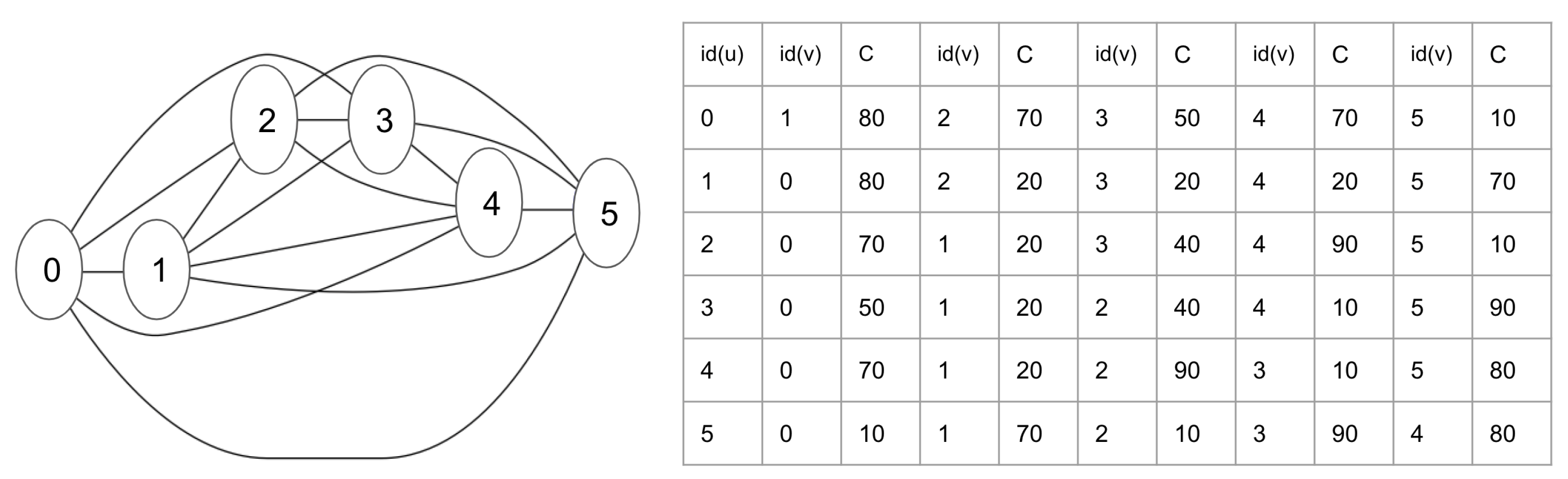
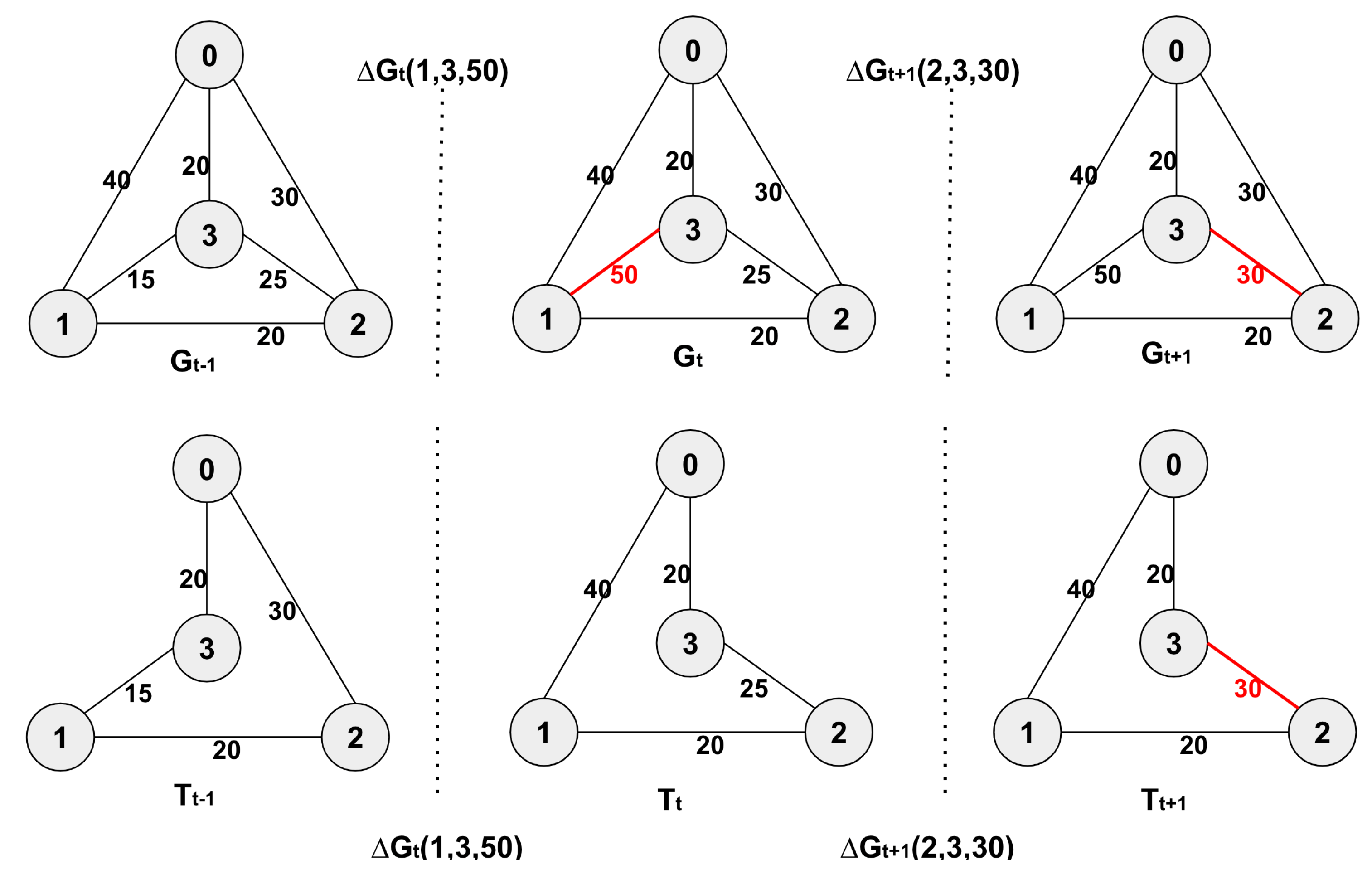
2.1. Time Evolving Graph

Processing time-evolving graphs is challenging due to the changing topology of the graphs. These challenges are discussed in a survey [21,22] where computation techniques on TEG are studied in three domains i.e., graph analytics, graph computing frameworks, and graph algorithms. As the changes in each graph happen frequently, not only the time taken to compute the graph will be expensive but it will even impact the performance of the underlying computing framework. Abdolrashidi et al. [23] have addressed this problem by proposing a partitioning algorithm for dynamic graphs in cluster computing frameworks. They have considered communication cost, the number of intra-node edges, and load distribution while determining the placement of the partitioned graph. However, it gets more challenging to determine a placement for newly arriving vertices in graph partitions. FENNEL [24] is a k-partitioning algorithm that takes decisions regarding the placement of newly arriving vertices in the graph. It uses a heuristic algorithm to place the new vertex in a partition that has either the largest number of neighbors or non-neighbors.

2.2. Traveling Salesman Problem

TSP is a well-studied problem in the field of graph computing. It has various applications in computer science and operation research. Hence, finding an optimal solution for TSP is challenging. In order to find a global optimal solution, various metaheuristic algorithms have been proposed. These algorithms are: $\left(1\right)$ Genetic algorithm [13,25], which finds fittest individuals that can generate new offspring in every generation, $\left(2\right)$ Simulated annealing [26], which finds approximate solution using the probabilistic technique, and several others such as $\left(3\right)$ Ant Colony Optimization [27], $\left(4\right)$ Particle Swam Optimization [28], and $\left(5\right)$ tabu search [29]. Hybrid algorithms [30] are even well studied in the literature, and they can further improve the accuracy and efficiency. There are many versions of the TSP algorithm. Three of them are Generalized TSP (G-TSP), Multiple TSP ( M-TSP), and Clustered TSP (C-TSP). In GTSP [9,10,11], the nodes of a complete undirected graph are partitioned into clusters, and the objective is to find a minimum cost tour passing through exactly one node from each cluster. Multiple TSP (MTSP) [12] consists of more than one salesman, and each salesman visits an exclusive set of vertices. In C-TSP [8], the group of cities must be visited contiguously in optimal and unspecified order. The real-world warehousing problem is an example that fits this problem definition. Many researchers [31] have also used the divide and conquer strategy to solve various applications of TSP. The main idea is to divide the solution space into sub-problems and then solve each sub-problem independently in parallel. In the current work, we have used the divide and conquer strategy to partition the graph and compute a TSP tour on only the affected partition.

2.3. Incremental Algorithms

In time-evolving graphs, incremental algorithms have been widely used for several graph problems such as pagerank, pattern matching, and the shortest path. Fan et al. [16] have designed incremental algorithms for various use cases in pattern matching such as sub-graph isomorphism, graph simulation, and bounded simulation. On the other hand, for the graph simulation model in pattern matching, Kao et al. [17] have proposed a distributed incremental algorithm. Desikan et al. [18] have used an incremental algorithm with a partitioning strategy to keep the changed and unchanged parts of the graph in separate partitions for the page rank problem. Bahmani et al. [19] used a probing approach to find the changed portion of the graph and compute the page rank. Anagnostopoulos et al. [20] have implemented an incremental algorithm for graph problems such as path connectivity (PC) and minimum spanning tree (MST), where the algorithm does not get notified about the changes. Similarly, Blelloch et al. [32] have designed an randomized incremental algorithm for the convex hull problem. Yuan et al. [33] have focused on a graph-coloring problem for an incremental approach, and it stores the intermediate results as the graph keeps on changing. Incremental algorithms have even been used for partitioning the graph incrementally [34].

2.4. Graph Partitioning

Partitioning algorithms aim to partition the graph in such a way that the majority of the computation can take place locally. The partitioning can be performed either on an edge (edge cut) or a vertex (vertex cut). An edge cut is a partitioning technique that evenly splits vertices to partitions such that the number of crossing edges is minimum. Another partitioning technique, vertex cut, mainly splits edges to partitions such that the number of crossing vertices is minimal. In real-world use cases, vertex cut is known to produce a more balanced partitioning result where the degree distribution in the graph follows a power law. While in vertex cut, the state of a vertex keeps on changing, edge cut is known to maintain data consistency [35]. Filippidou et al. [36] have designed a full TEG partitioning strategy where the systems process the changes simultaneously. They have even proposed an online node placement algorithm that heuristically places the incoming nodes on the fly. Furthermore, a Compressed Spanning Trees (CST) helps to fetch all the statistical analytics from the summary created by a compact summary structure. CST helps to do partition on the fly whenever required in real time. Therefore, it is important to note that the performance of the cluster directly depends on the way of the partitioning and placement strategy of the graph on computing nodes.

Another partitioning approach has been proposed by Abdolrashidi et al. [23] for dynamic graphs with a cost-sensitive strategy. In their strategy, they have considered several factors such as load distribution among computing nodes, the number of intra-node edges, and communication cost. In order to handle graph update events, they have proposed incremental algorithms based on cost heuristics. Tsourakakis et al. [24] have proposed an objective function for their graph portioning strategy that is composed of two costs: (i) cost of the edge cut and (ii) cost of the sizes of individual clusters. There are three orders of streaming techniques: random, BFS, and DFS. They have proposed a k-partitioning algorithm that aims to place new vertices, However, the location of the vertex cannot be changed again. Moreover, a greedy strategy is used to implement another kind of streaming algorithm, which is called the one-pass streaming algorithm. The vertex is assigned to a partition such that the objective function is maximized for a k-graph partitioning problem.

3. Algorithms

3.1. Problem Definition

In our problem definition, as explained in our previous works [14,15], G is a complete, undirected graph. In a TSP problem, the tour is computed on a graph $G(V,E)$, where V is the set of vertices and E is the set of edges. The goal is to compute a tour T where each vertex in the graph is visited exactly once such that the total traveling cost is minimum. The total traveling cost of a tour T is the sum of the weights of all the edges in tour T. Now, the problem definition for solving TSP on TEG is different. For every update event, we have to find the minimum TSP tour T in each time interval. The TEG instance at time t is denoted by $G_t=\{V,E\}$. The cost of an edge $(u,v)$ is defined as $C(u,v)$, where u and v are two vertices. We only consider one type of update event i.e., change in edge weight, and we have assumed there can be only one update event for each time interval. Therefore, the update event is denoted by $\Delta G_t(u,v,C(u,v))$, which means the weight of the edge $(u,v)$ is changed to $C(u,v)$ at time interval t.

To explain the above problem definition, we will use same Figure 1 as used in our previous works [14,15]. For example, the first row of images of Figure 1 illustrates an update event $\Delta G_t=(1,3,50)$ and $\Delta G_{t+1}=(2,3,30)$ at time interval t and $t+1$, respectively. This means that the weight of vertices 1 and 3 is updated to 50 at time interval t, and similarly, the weight between vertices 2 and 3 is changed to 30 at time $t+1$. The second row of images of Figure 1 shows the respective TSP tours of each graph. Our objective is to compute the minimum TSP tours {0, 3, 1, 2, 0}, {0, 3, 2, 1, 0} and {0, 3, 2, 1, 0} for every time interval. To achieve this objective, we have proposed an incremental algorithm, which is discussed in the next subsection.

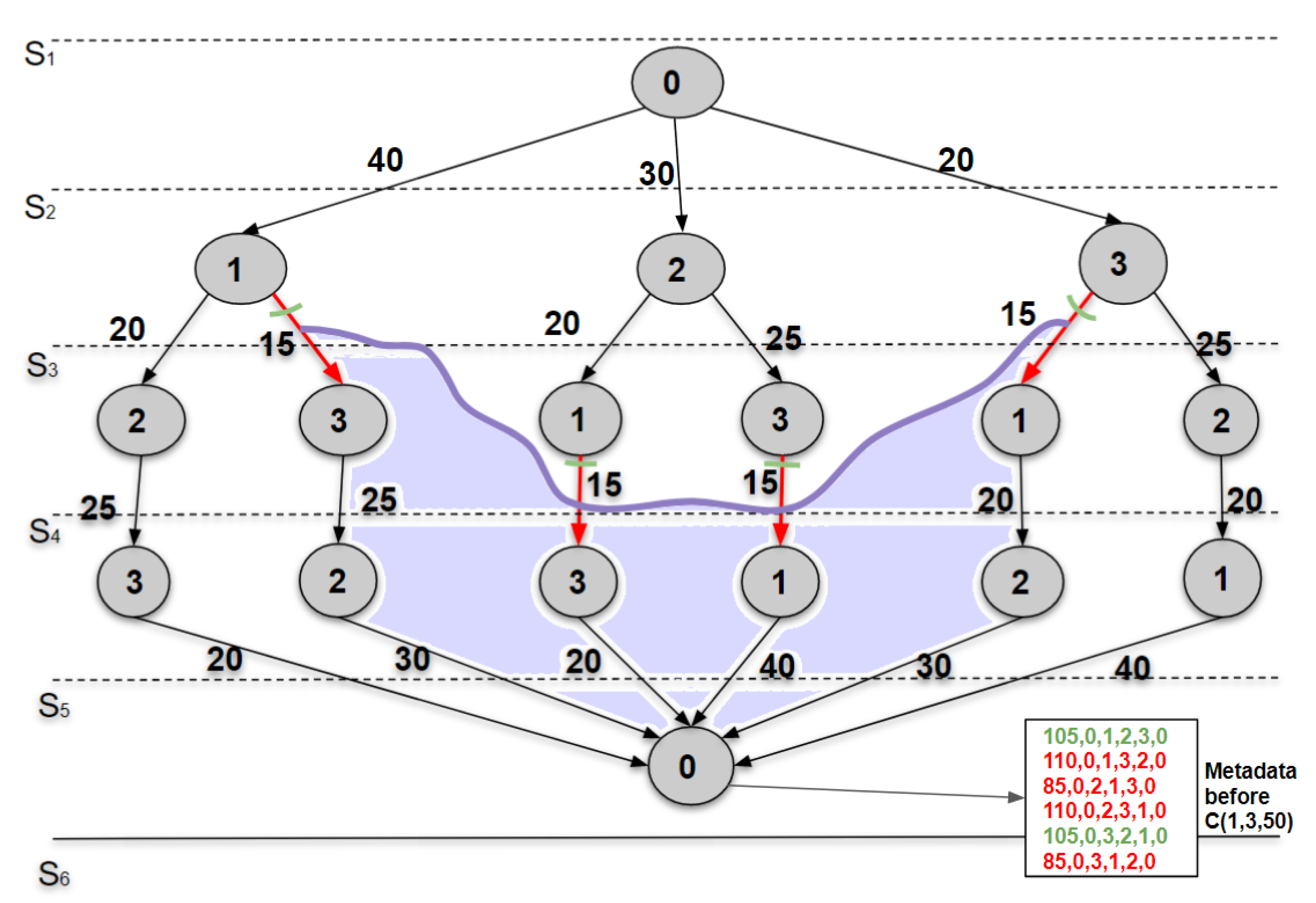
3.2. Incremental Algorithm

In our previous work, the inputs of an I-TSP and Ig-TSP algorithm include the complete graph, the results from the previous time interval, and the update event. The objective is to reduce the amount of recomputations in the updated graph for the current time interval. All the TSP tours of a graph are represented by a search tree [14], as shown in Figure 2. Each tour in a search tree will be a path. The intuition of I-TSP is to only recompute the paths that are affected by the update event. The pseudocode is shown in Algorithm 1. I-TSP and Ig-TSP differ from each other in their method of propagation. Where the I-TSP algorithm propagates messages to all the neighbors, Ig-TSP being a greedy algorithm that propagates only to the closest neighbor.

Algorithm 1: Incremental distributed TSP Algorithms: I-TSP and Ig-TSP [14].

Input:$\Delta G_t(u,v,C(u,v))$, pathList. Output: A TSP tour, T 1: preProcessing(pathList) 2: $id\left(source\right)⟶sendMessage(U,initialVertexMessage)$ 3: for vertex v do                                                ▹ Parallel for loop 4:     for message do 5:         if ($S\ne 1\&\&message.last\ne id\left(v\right)\&\&message.length\ne n+1\&\&message\left[path\right]\not\subset validPathList$) then 6:            if $id\left(v\right)\notin message$ then 7:                updateMessage(message) 8:            end if 9:            if (mode == brute) then 10:                propagateAll(message) 11:            else 12:                propagateGreedy(message) 13:            end if 14:         else 15:            sendMessage(id(source), message) 16:         end if 17:     end for 18:     computeTSPTour() 19: end for 20: function preProcessing(pathList) 21:     for path in pathList do 22:         for p in path do 23:            if $p\left[j\right]==id\left(v\right)\&\&\left(p\right[j-1\left]orp\right[j+1]==id(u\left)\right)$ then 24:                invalidPathList += path 25:            else 26:                validPathList += path 27:            end if 28:         end for 29:         for path in invalidPathList do 30:            for p in path do 31:                if (($p\left[j\right]==id\left(v^{\prime }\right)orid\left(u^{\prime }\right))\&\&j>1$) then 32:                    truncatedPathList += path.sublist(1,j) 33:                end if 34:            end for 35:         end for 36:     end for 37:     for Y in truncatedPathList do 38:         if (y.last = = id(v)) then 39:            initialVertexMessage += y 40:         end if 41:     end for 42: end function

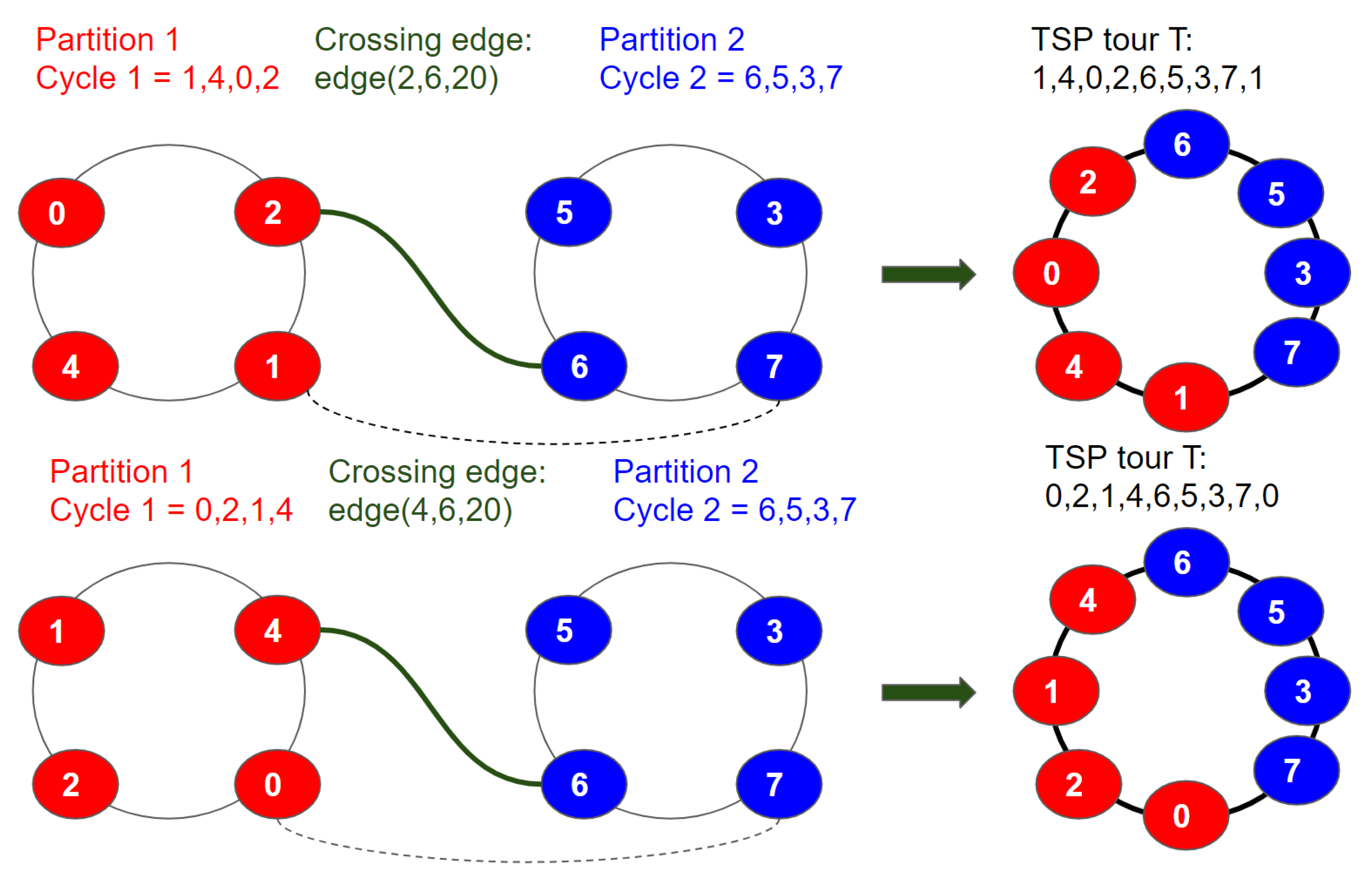
3.3. Graph Partitioning Algorithm

The intuition of a partitioning algorithm is to localize the computation on a partition where an update event has occurred. Hence, recomputing a partial TSP tour on an affected partition instead of recomputing the whole graph will significantly reduce the computation time and the messages sent. After P-TSP/Pg-TSP computes a partial TSP tour on each partition, these tours are connected to obtain a full-length TSP tour. To implement this intuition, we have three main steps: (1) partition the graph, (2) recompute a partial TSP tour, and (3) connect the partial tours of each partition. The graph that will be used as reference is shown in Figure 3. The connecting process is shown in Figure 4. Finally the resultant graph for all partitioning strategies is shown in Figure 5

Step 1: Graph Partitioning: The input graph is partitioned to sub-graphs to reduce the communication cost in the distributed environment. In our problem definition, update event affects only one edge, and hence, the total computation time is reduced because recomputation will take place in at most one partition. A graph can be partitioned based on various constraints. We will discuss these constraints in detail in the next section.

Step 2: Recompute TSP tour: Whenever an update event occurs, it will affect only two vertices of the partition. These two vertices can either be present in the same partition or in a different partition. If the affected vertices are in the same partition, then I-TSP or Ig-TSP will be used to compute the TSP tour on that partition. The recomputed tour is later connected with a partial tour of other partitions. If the vertices affected by the update event are in different partitions, we do not need to recompute at all and connect previously computed tours with a new minimum edge across partitions, which is explained in the next paragraph.

Step 3: Connecting partial TSP tours: The changed edge will affect a maximum of two partitions of the graph. Therefore, the connecting process will also take place between two partitions. After step 2, we will have two recomputed partial tours of affected partitions. We propose an algorithm to connect n tours into one tour. The intuition of the algorithm is to cut each tour in a linear sequence and then connect them to construct a new tour. So, the first step is to find the cutting point, and the second step is to construct the tour. Figure 4 illustrates the connecting algorithm for a graph with two partitions.

The pseudocode for both of our partitioning algorithms is shown in Algorithm 2. I-TSP and Ig-TSP are the underlying algorithms for partitioning algorithms. The propagation of I-TSP and Ig-TSP is shown in  [14]. The input to the algorithm is an update event and a pathList from previous iterations. The graph is partitioned in line 1. If u and v of $\Delta G_t(u,v,C(u,v))$ are present in the same partition (line 2), then depending on the mode, I-TSP (line 4) and Ig-TSP (line 6) are used to recompute the TSP tour on that partition. If both u and v are in different partitions, then the minimum edge is chosen (line 9) to connect the partitions (line 11).

Algorithm 2: Partitioned TSP Algorithms: P-TSP (Based on I-TSP) and Pg-TSP (Based on Ig-TSP).

Input:$\Delta G_t(u,v,C(u,v))$, pathList. Output: A TSP tour, T 1: Partition the graph using edge attribute, node size attribute, or k-means method. 2: if u and v are in the same partition then 3:     if mode == brute then 4:         compute T using the I-TSP algorithm                ▹ P-TSP algorithm 5:     else 6:         compute T using the Ig-TSP algorithm                ▹ Pg-TSP algorithm 7:     end if 8: else 9:     Pick minimum weight edge across partitions CE(u${}^{\prime }$,v${}^{\prime }$). 10: end if 11: Connect tours of each partition by connecting CE(u${}^{\prime }$,v${}^{\prime }$).

3.4. Graph Partitioning Constraints

In this paper, we have mapped different partitioning methods to our problem definition and implemented them to compare which method can give better results for the TSP algorithm on TEG. To better understand our partitioning methods, we have considered Figure 3 as our example, which is a fully connected graph comprising of six vertices. The adjacency list for the graph is also shown. The three partitioning constraints used in this paper are as follows:

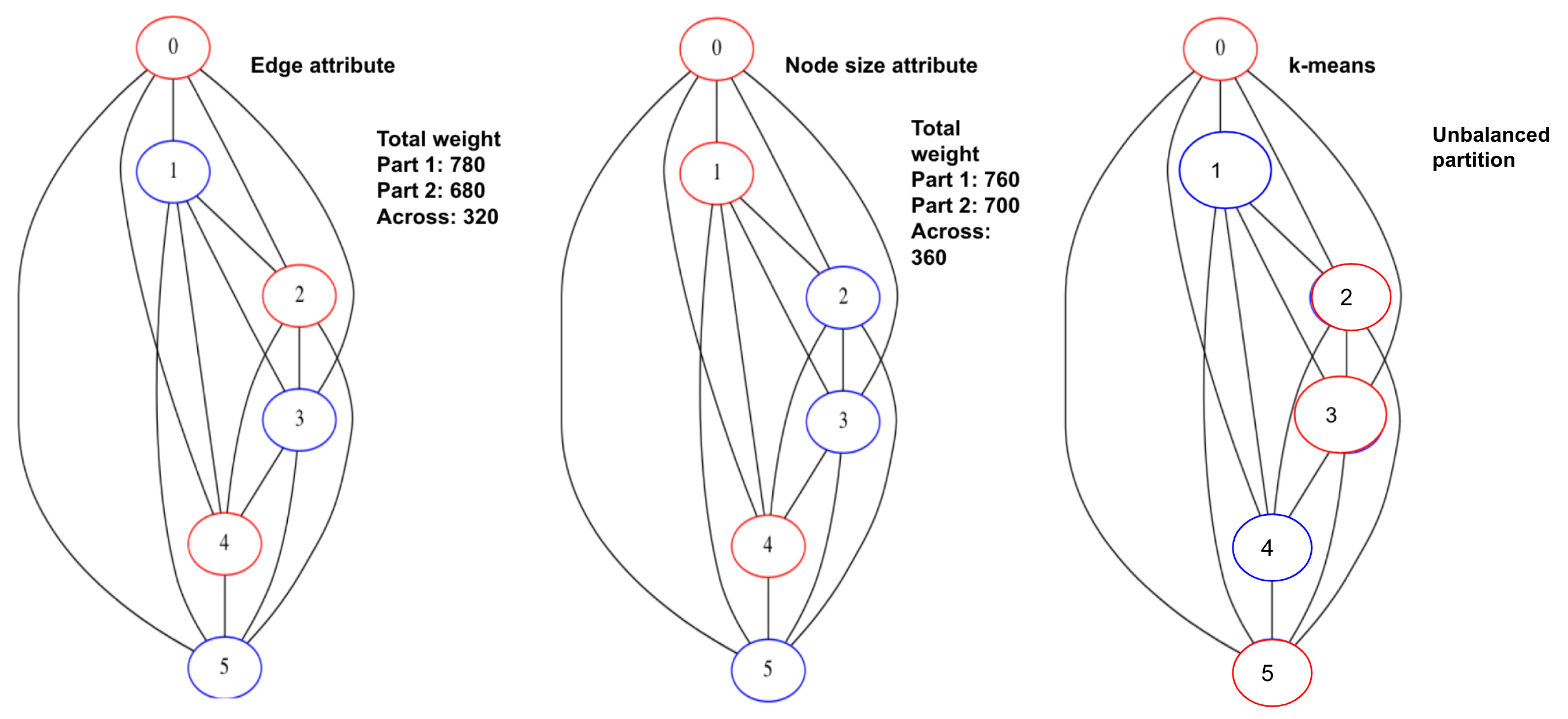
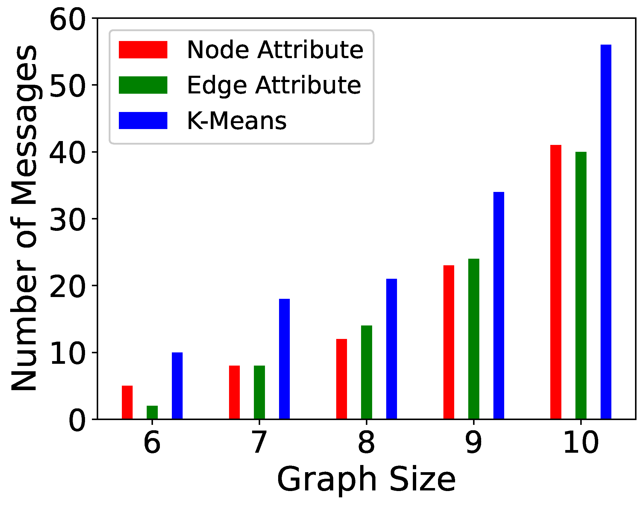
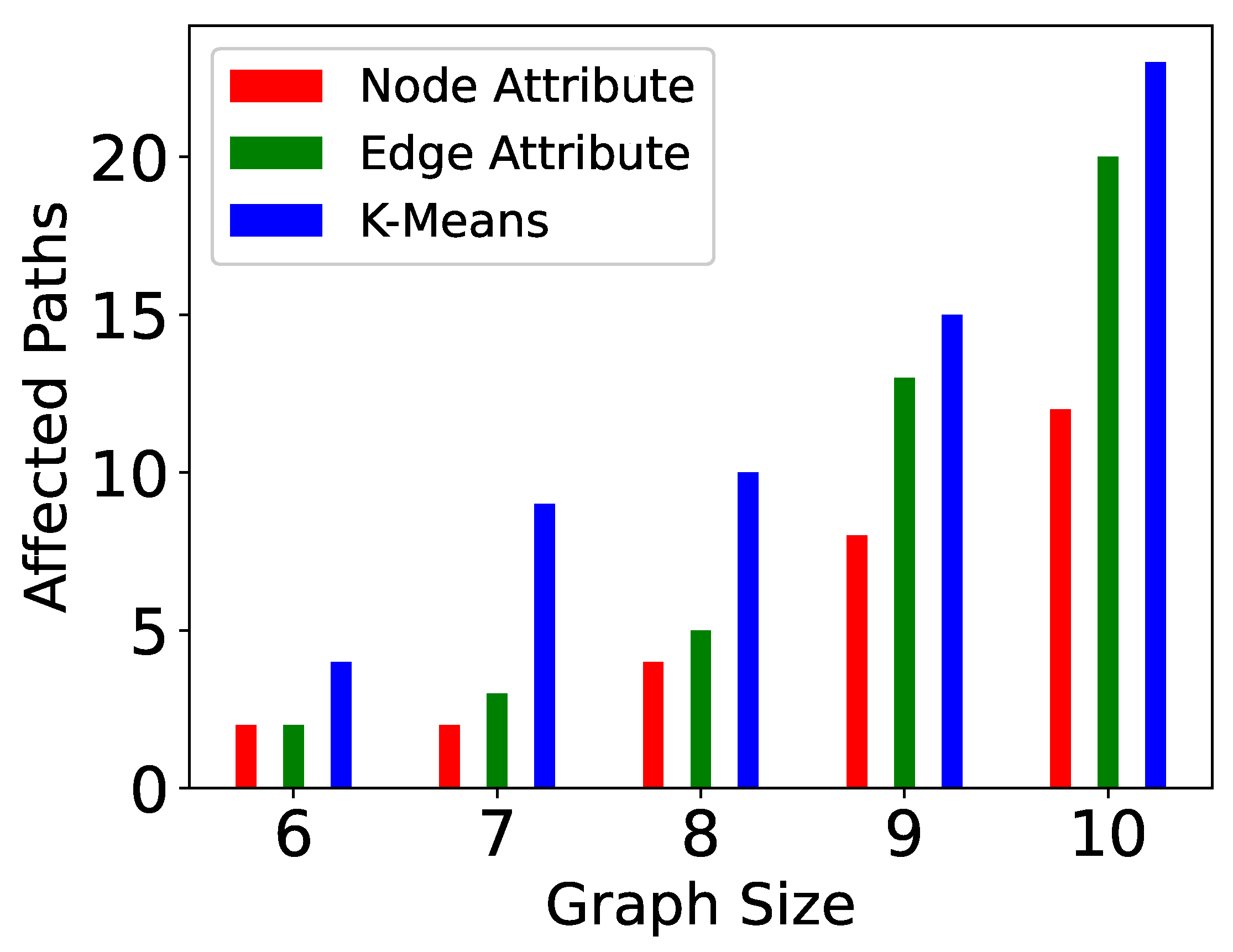
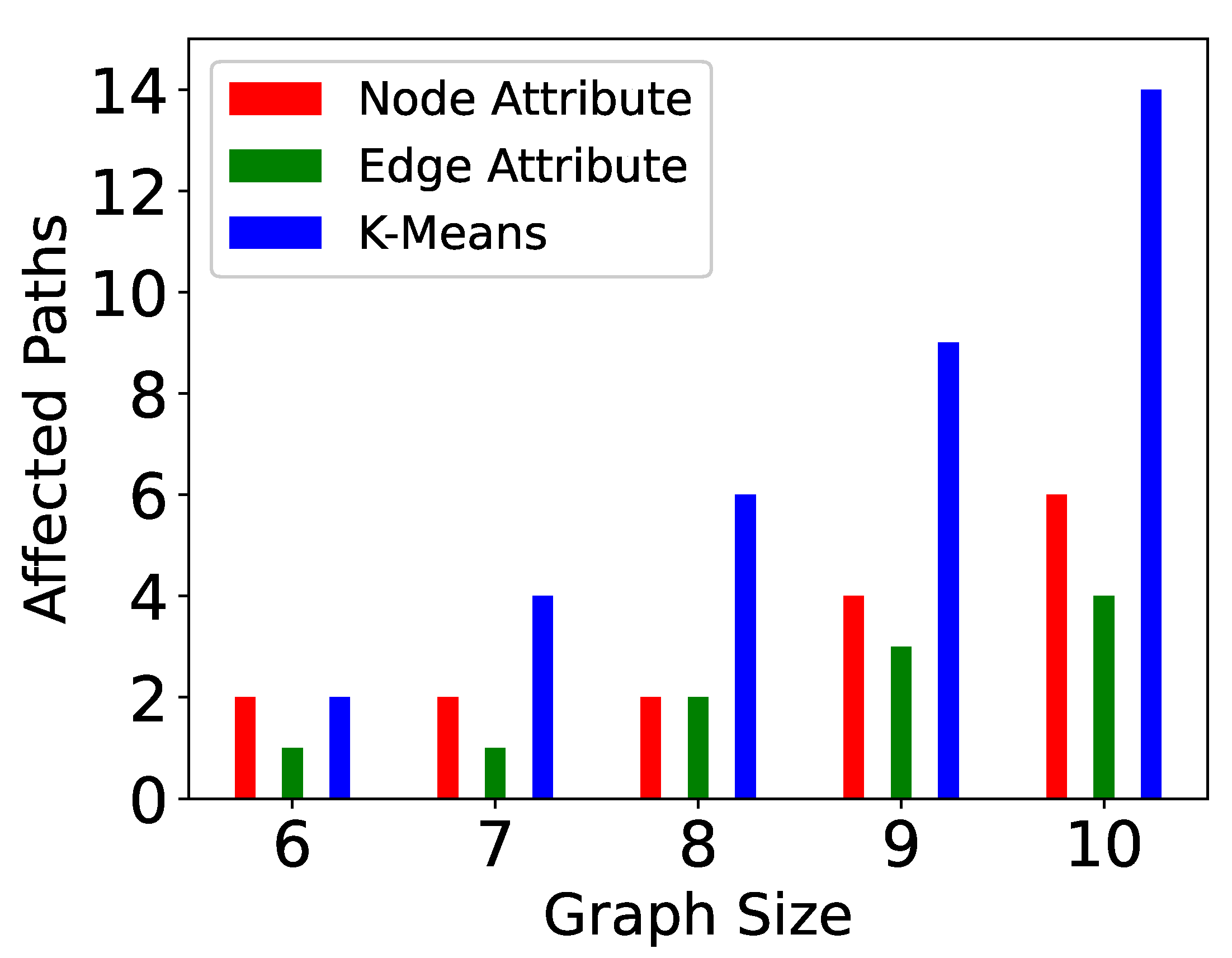
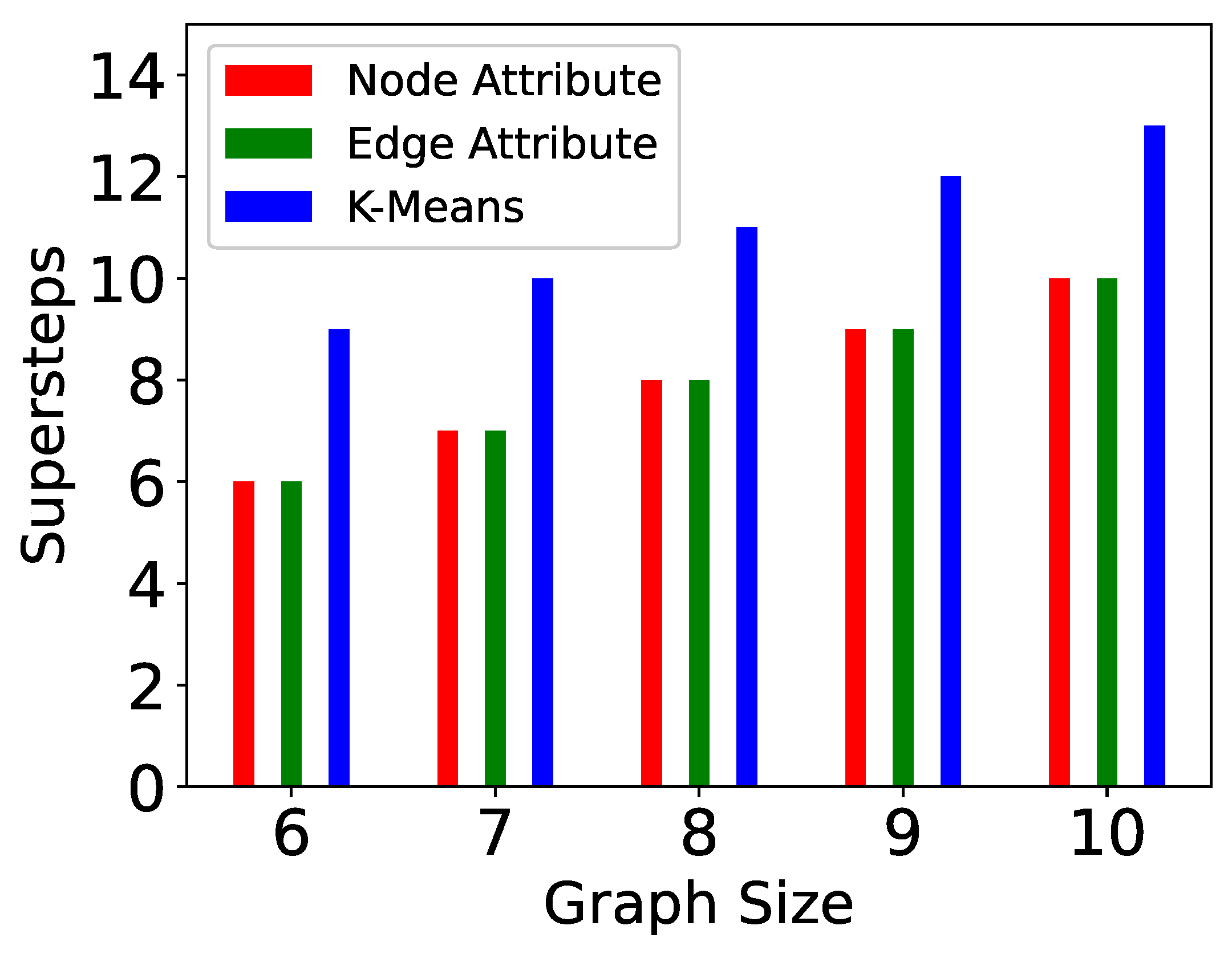
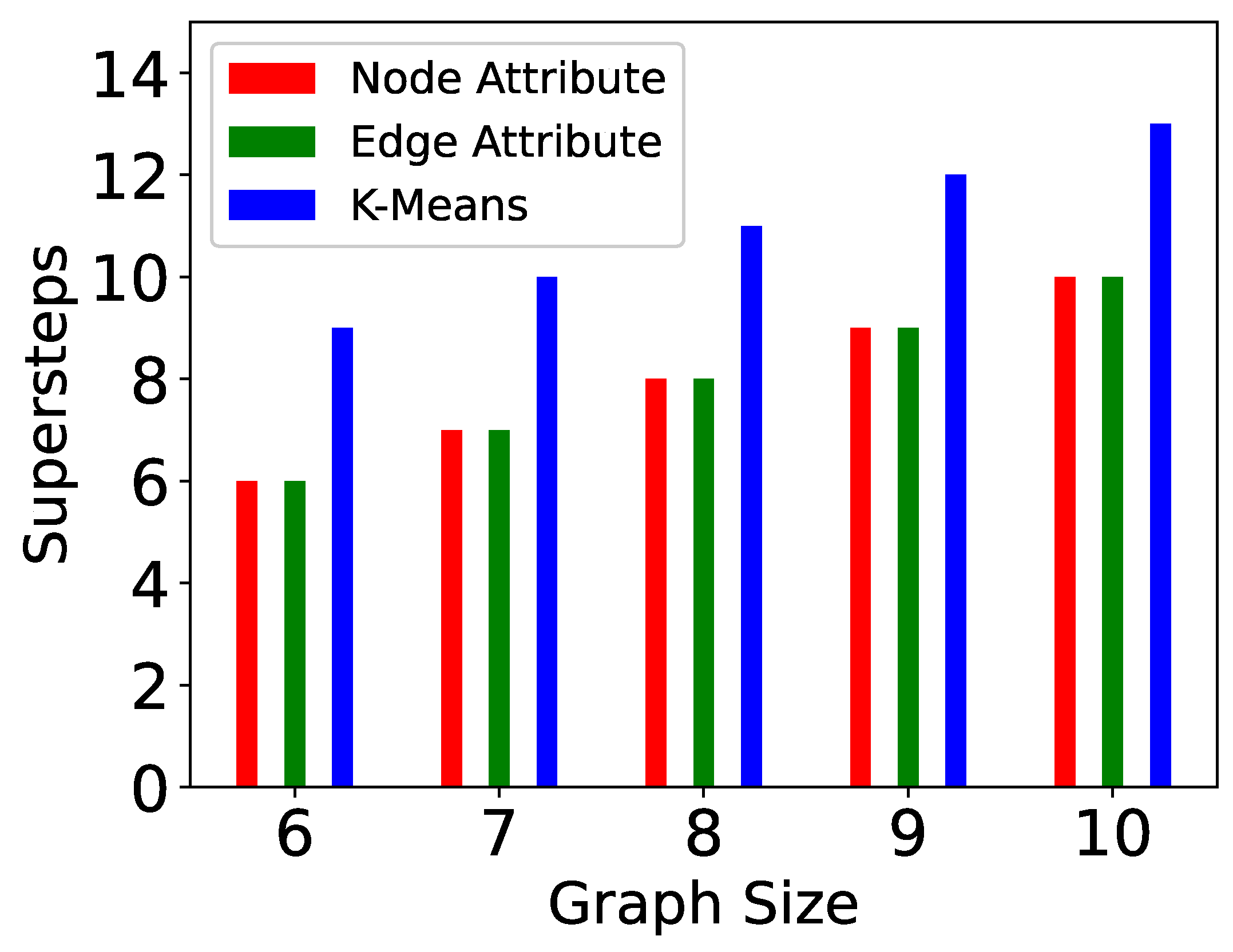
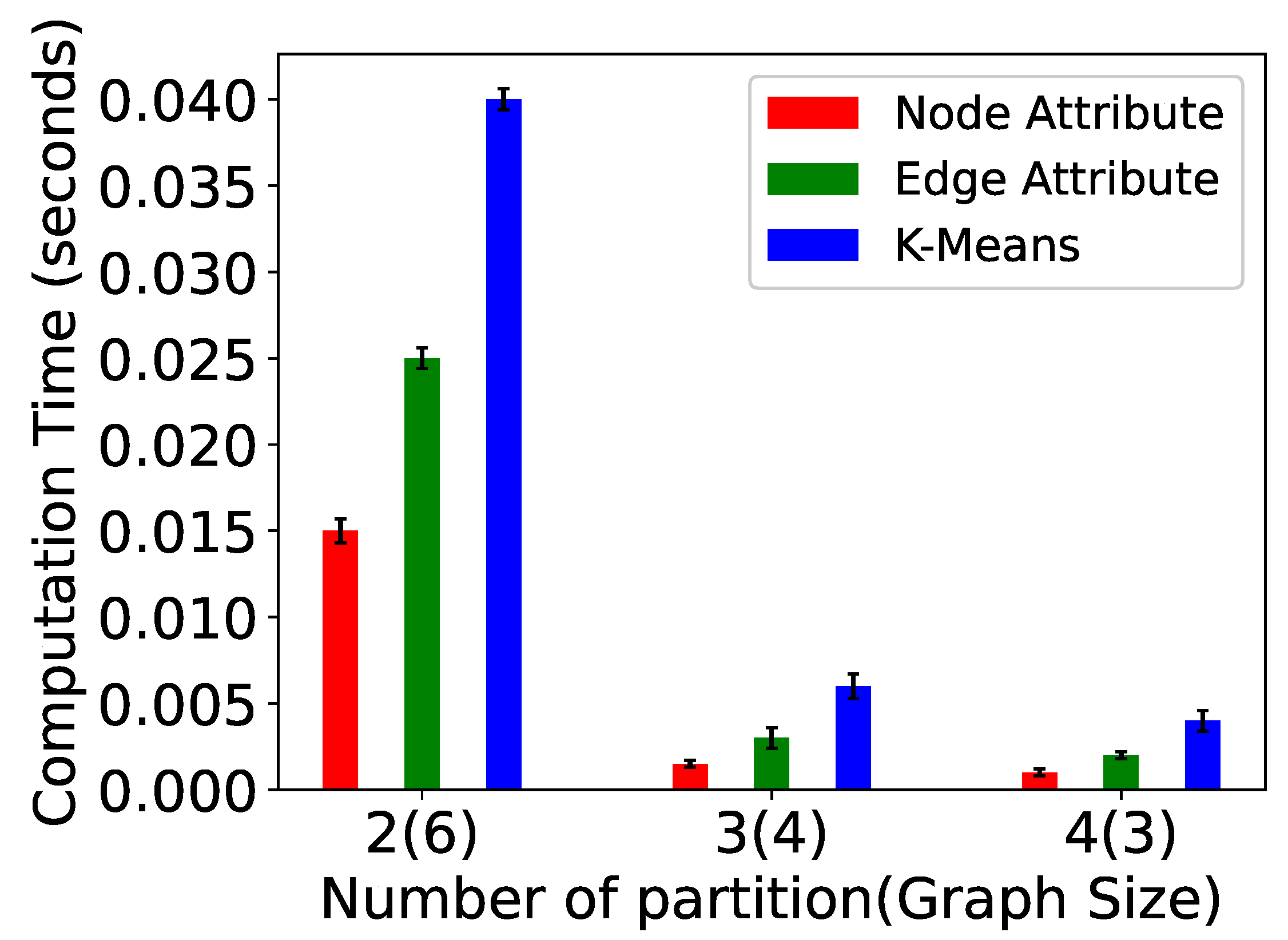
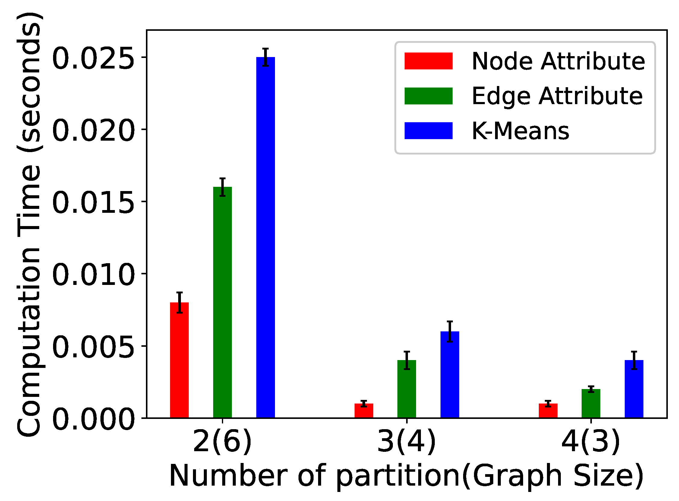
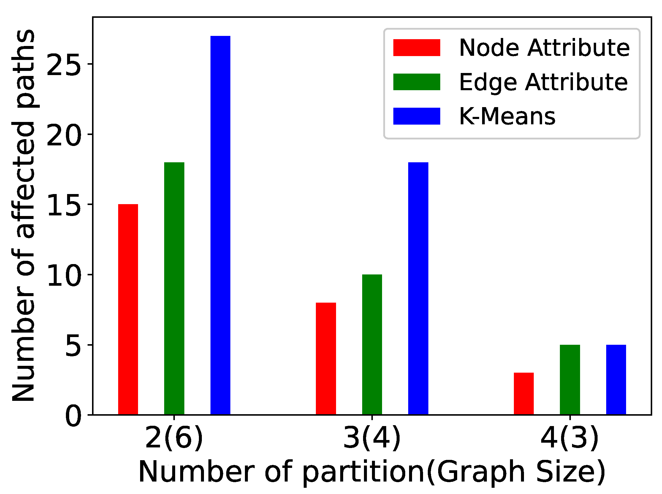
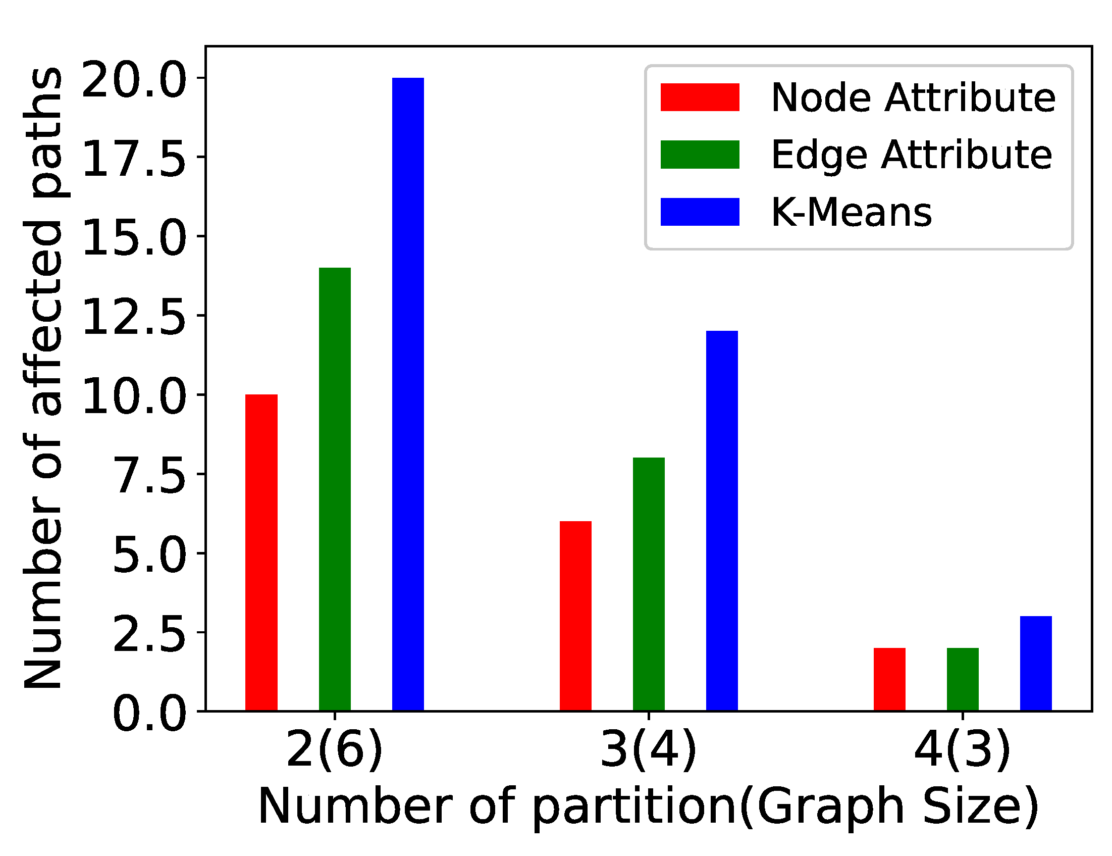
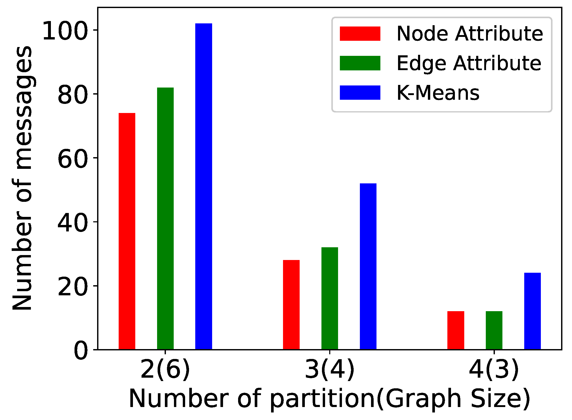
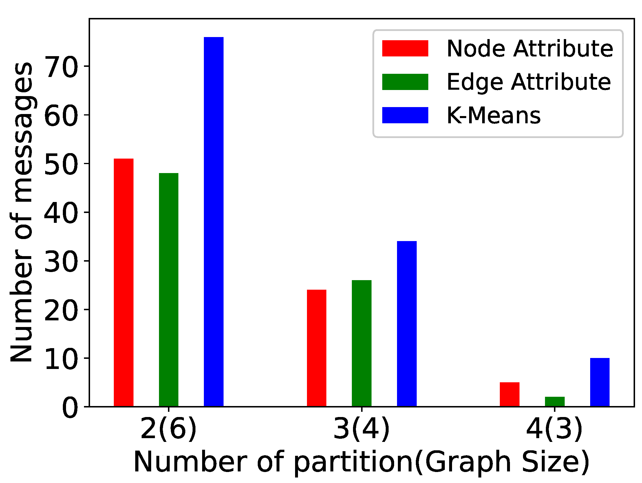
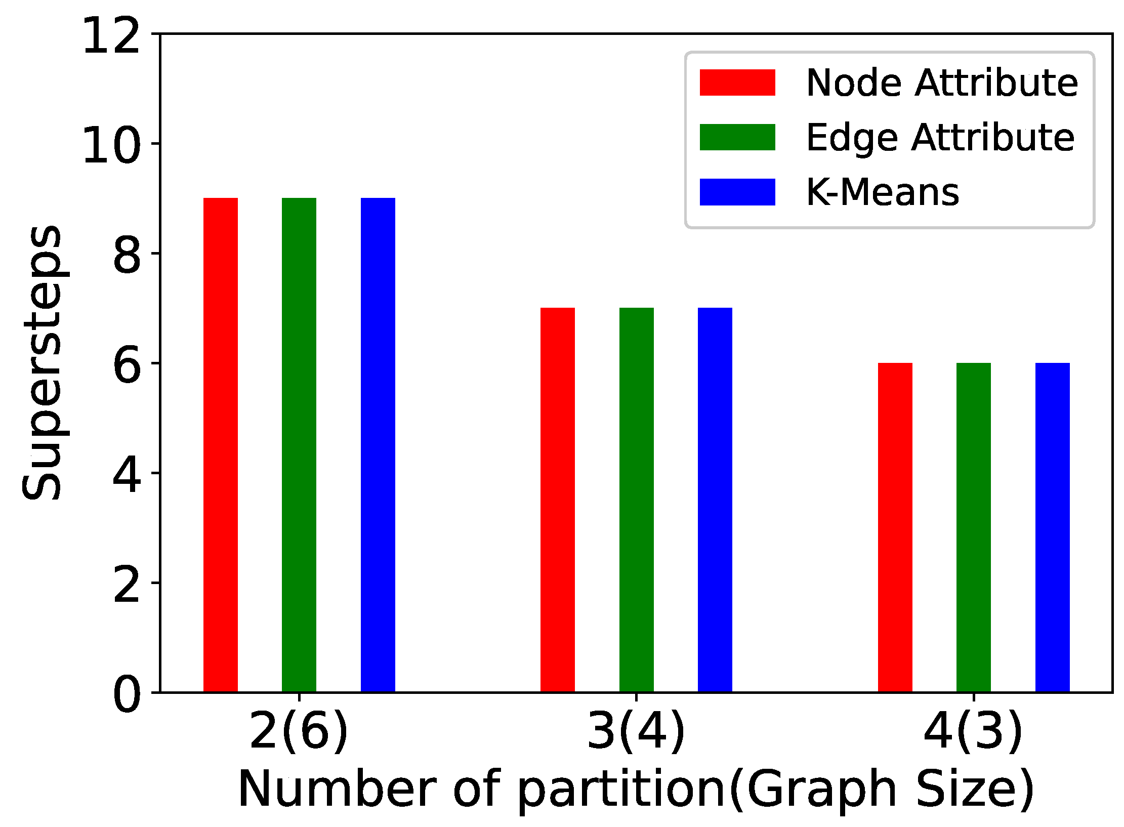
• Vertex size attribute partitioning (NP-TSP): The vertex size is defined as the total weight of outgoing edges from a vertex. This method focuses on balancing the partitions. The vertices in a partition are added in such a way that the difference between the total weight of each partition is minimum. For example, in Figure 5, the total difference between both the partitions is less than the edge attribute method. This is the baseline partitioning method without any constraint.
• Edge attribute partitioning (EP-TSP): In this method, the graph is partitioned in such a way that the total weight of edges across the partitions will be minimum. The intuition behind this method is to minimize the cost of connecting the sub-tours when the number of partitions is higher. For example, in Figure 5, the total weight of edges across the partition is 320. Therefore, this method can save computation cost for graphs with a higher number of partitions because if the weight across the partition is already minimized, then the probability of getting a nearly optimal tour increases. This partitioning strategy avoids a higher cost edge in the partition.
• k-means partitioning (KP-TSP): The k-means method is an iterative partitioning algorithm where k random vertices are placed as a centroid in different partitions. In each partition, the vertices close to centroids are added iteratively. The intuition behind this method is to keep closer vertices together. This method is also useful for a larger graph with a higher number of partitions. In Figure 4, the centroids for both partitions are randomly chosen as 1 and 4, respectively. Partition 1 contains vertices 2 and 5 because they are closer to vertex 1, and partition 2 contains vertices 0 and 3 because they are closer to vertex 4.

4. Complexity Analysis

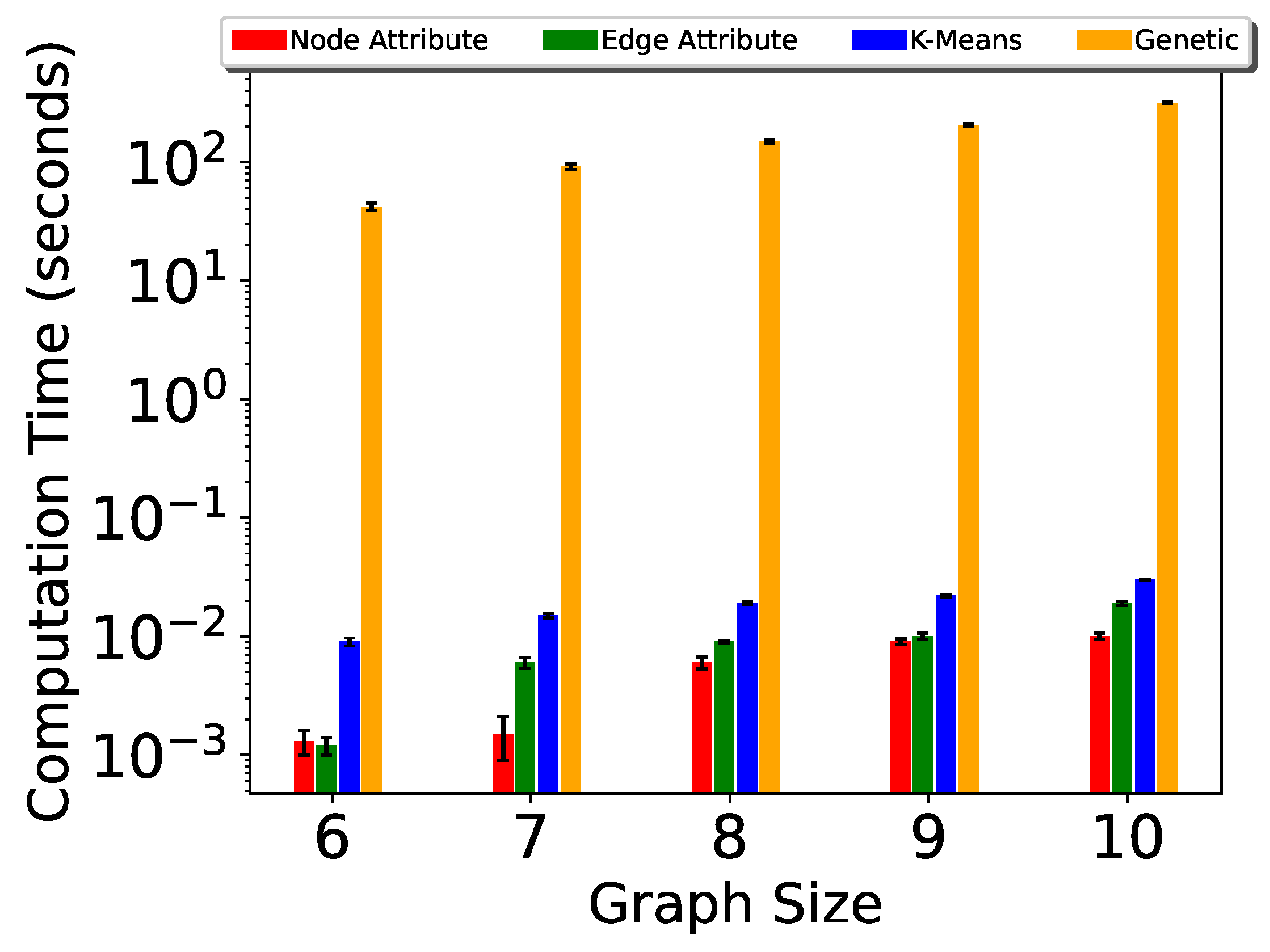
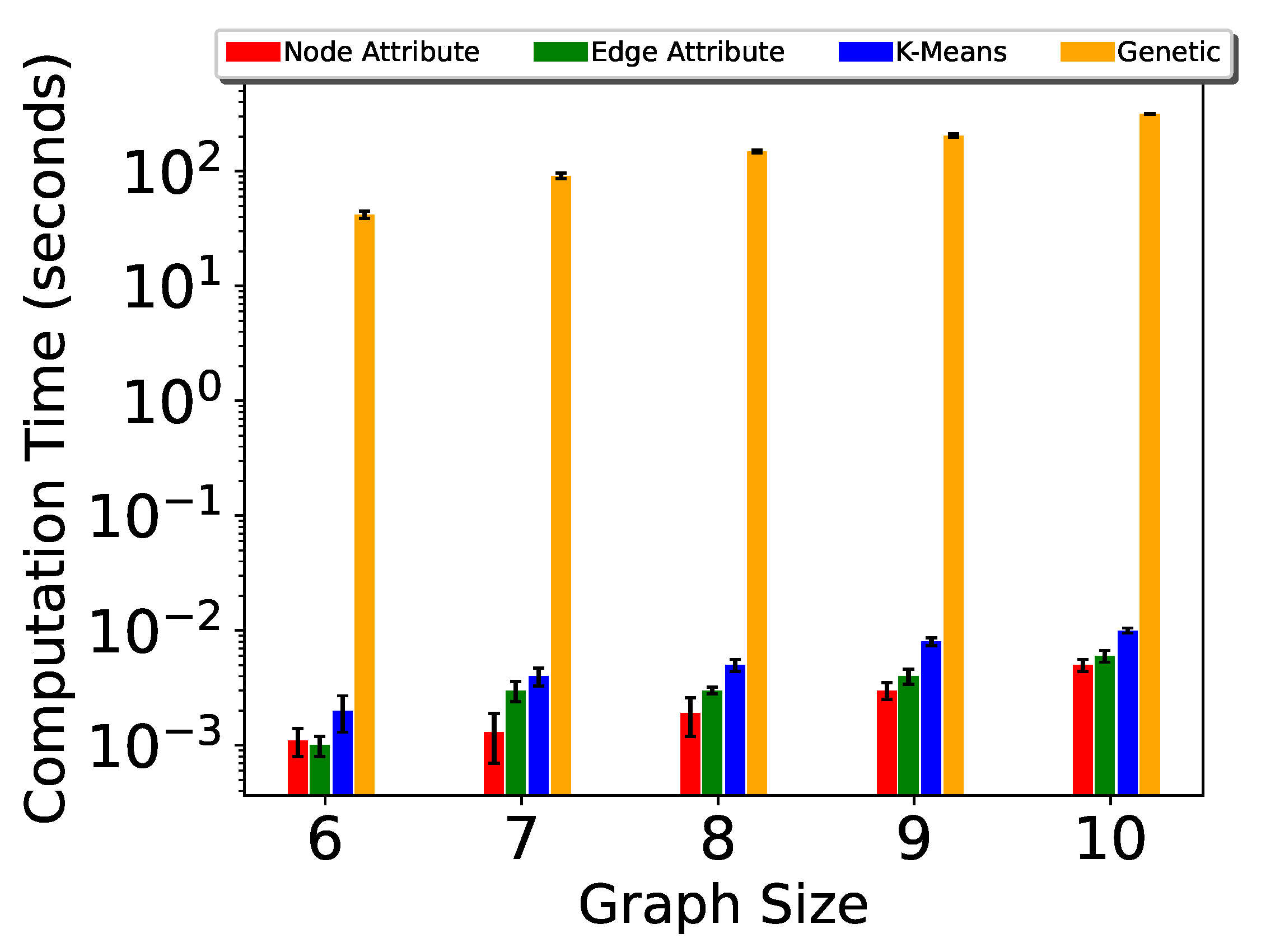
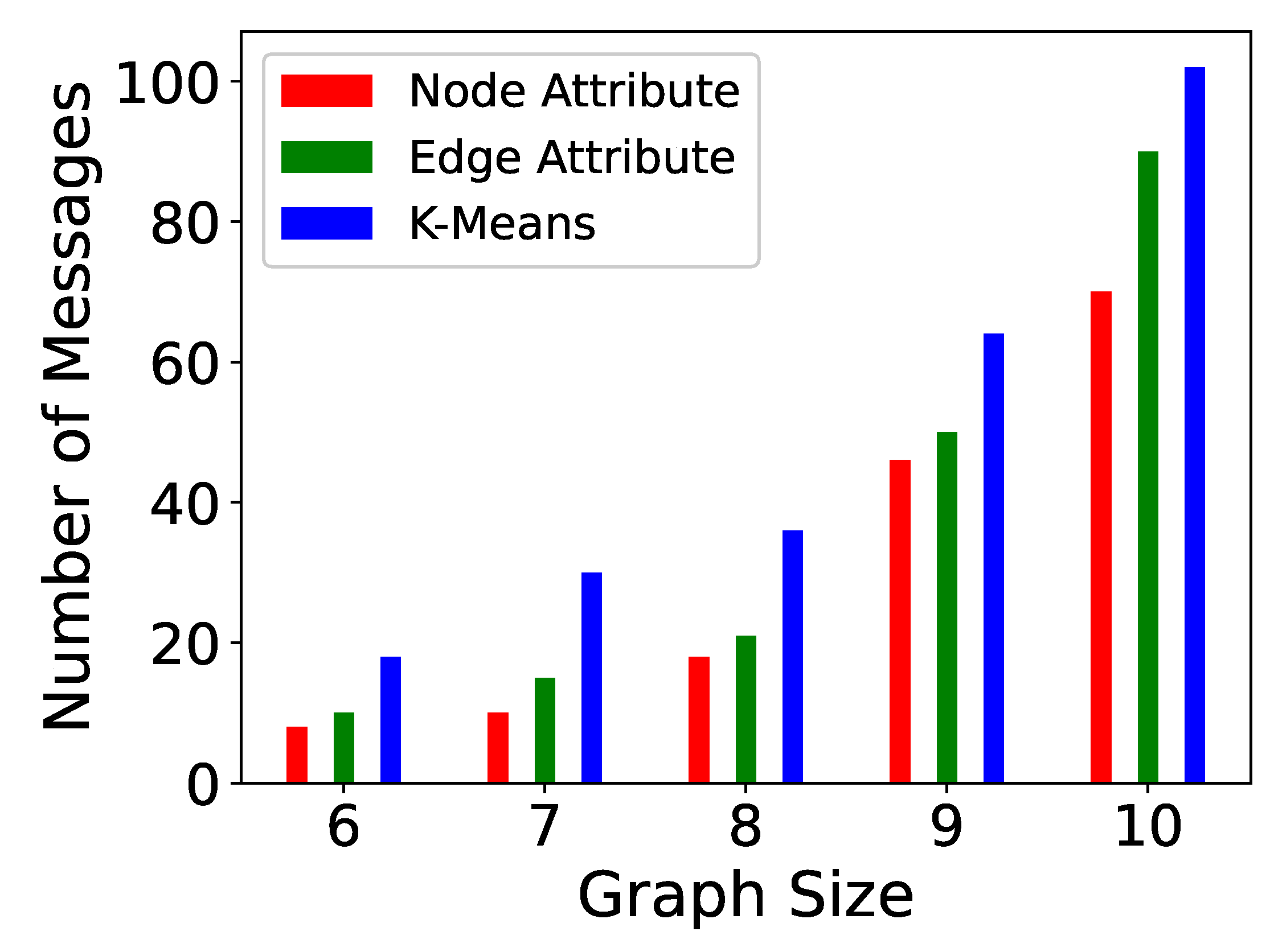
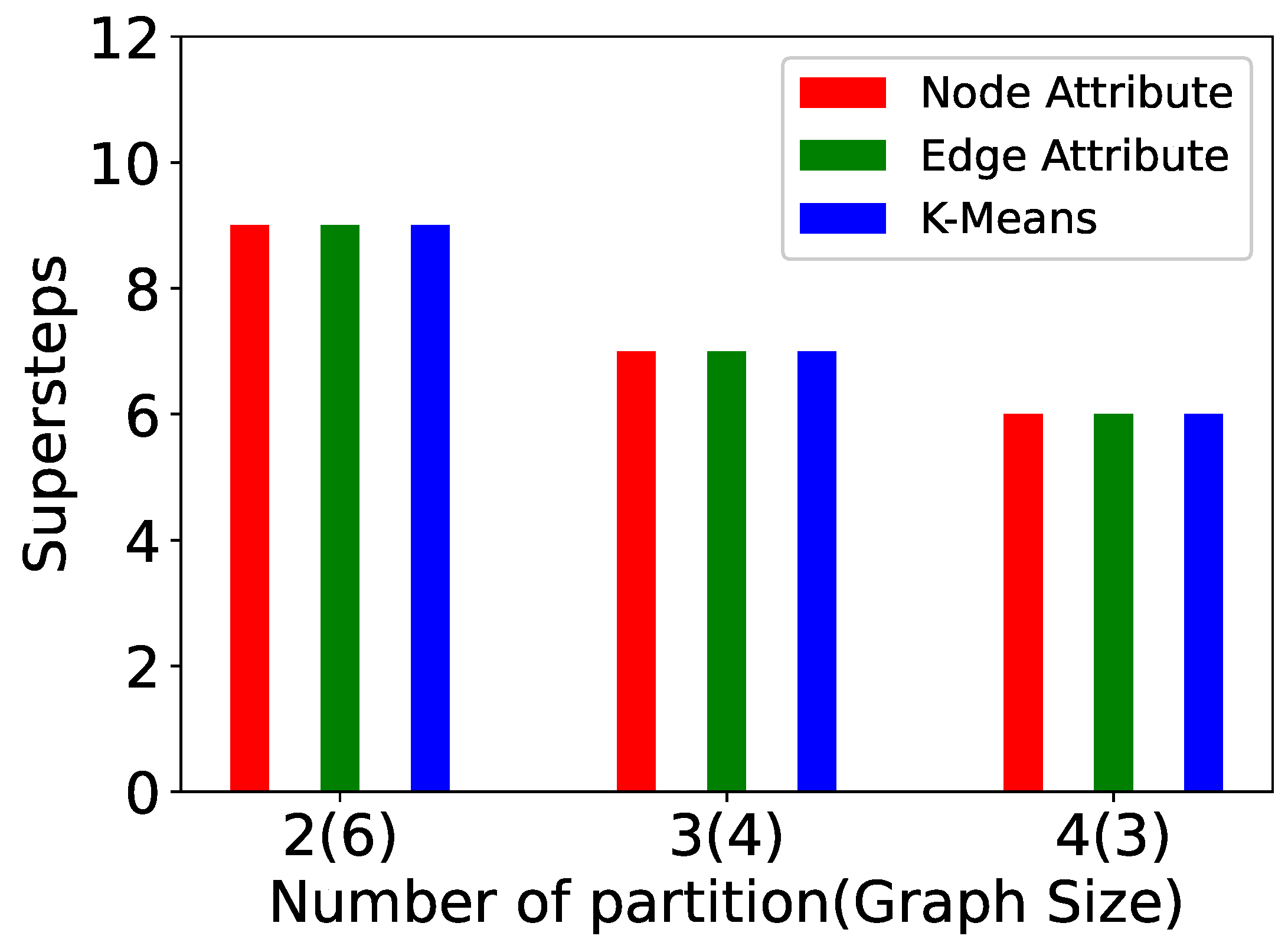
In the TSP algorithm, the computation time depends on the number of vertices in graph. Even if the algorithm is executed in a distributed way, the number of messages sent to traverse all the permutations of TSP tours will be directly proportional to the number of vertices. In an incremental algorithm, the computation begins from the previous result. The previous result in our algorithm is the set of full-length paths traversed in the previous iteration. In order to measure time complexity, we measure how many less messages will be sent in an incremental algorithm. To calculate that, we will first show the number of messages for the distributed TSP algorithm, which is a distributed implementation of the TSP algorithm. The summary of previously proposed algorithms and the partitioning algorithm is shown in

Table 2. Summary of complexity analysis.

Algorithm	Paths	Messages
Distributed-TSP (D-TSP)	$(n-1)!$	$n(n-1)!$
Incremental-TSP (I-TSP)	$2/3\ast (n-1)!$	$2n/6(n-1)!$
Partitioning-TSP (P-TSP)	$(2/3\ast (n-1)!)/k$	$(2n/6(n-1)!)/k$

.

Lemma 1.

Number of paths P explored in distributed TSP algorithm is $(n-1)!$ and the total number of messages sent to compute those paths will be $n(n-1)!$.

Proof. 

If we examine Figure 2, each vertex will send messages to all the neighbors in a complete graph. Since one vertex is marked as a source vertex, the total permuted paths possible will be $(n-1)!$. Now, to compute those $(n-1)!$ paths, messages will be sent in each superstep. The length of the path will be $n+1$ because each path begins and ends in the source vertex. To compute the path of length $n+1$, a total of n messages will be sent, which is equivalent to the number of edges in the path. Hence, the total number of messages sent will be $n(n-1)!$ □

Lemma 2.

The number of paths P explored in the I-TSP algorithm is $2/3\ast (n-1)!$, and the maximum total number of messages sent to compute those paths will be $2n/6(n-1)!$

Proof. 

From our experimental evaluation, we have observed that for any changed edge, the total affected paths will be 2/3 of the total number of permuted paths in the distributed TSP algorithm. Hence, the number of total permuted paths for I-TSP will be $2/3\ast (n-1)!$. The number of messages sent to compute these affected paths depends on the location of changed edge in the path. If the changed edge occurs in the beginning of the path, the maximum number of messages sent will be $n-1$, and if the changed edge is at the end of the path, the minimum number of messages sent will be 1. The average number of messages sent in the whole computation will be $n/2$. Hence, the average number of messages sent to compute $2/3\ast (n-1)!$ paths will be $2n/6(n-1)!$. □

Lemma 3.

The number of paths explored in the P-TSP algorithm is $(2/3\ast (n-1)!)/k$ and the maximum total number of messages sent to compute those paths will be $(2n/6(n-1)!)/k$, where k is the number of partitions in the graph.

Proof. 

For the P-TSP algorithm, the complexity depends on the number of partitions and the number of messages. Since the underlying algorithm for P-TSP is the I-TSP algorithm, the number of affected paths will be the total number of paths in I-TSP divided by the number of partitions. Similarly, the number of messages will be divided by the total number of partitions. Hence, the average number of messages sent to compute $(2/3\ast (n-1)!)/k$ paths will be $(2n/6(n-1)!)/k$ □

5. Experiments

As discussed in problem definition, the graph in our experiments is complete and undirected. Due to the computation complexity, the graph size used in our experiment ranges from six to 12 vertices. We have used a vertex-centric framework named Graph Processing System (GPS) [37] by Stanford to implement our proposed algorithms. The server used for experiments is AMD Opteron 6282 SE CPU (16 cores and 2.6 GHz). The evaluated algorithms are P-TSP, Pg-TSP, and Genetic Algorithm [25] (only computation time). The three partitioning objectives used to partition the graph are vertex size attribute (balanced partition), edge attribute (min cut partitioning), and k-means (nearest neighbor approach).

The computation time for P-TSP and Pg-TSP is shown in Figure 6 and Figure 7. The three partitioning strategies—vertex attribute, edge attribute and k-means—are shown in red, green, and blue color, respectively. The k-mean strategy takes the maximum amount of time because the number of nodes in partitions is not the same. For example, in six vertex graphs, the two partitions consist of two vertices and four vertices, respectively. The computation time is bounded by the number of vertices and by the update event. If the update event takes place in a smaller partition, then it will be faster; otherwise, the larger partition will increase the computation time. Similarly, for edge attributes, the computation time depends upon the location of the update event in a graph.

The computation time is directly proportional to the number of messages sent. If the update event takes place in a partition where the number of vertices is more, then more messages will be sent to complete the reconstruction of the affected sub-graph. The number of messages sent in P-TSP and Pg-TSP for three partitioning strategies is shown in Figure 8 and Figure 9. The total path affected or computed to reconstruct the affected graph is shown in Figure 10 and Figure 11. The trend is the same as the computation time and the number of messages sent. If more paths are affected, then more messages will be sent to complete those paths, and hence, more computation will be taken. Figure 12 and Figure 13 show the number of supersteps taken to complete the computation of the TSP tour after an update event. The number of supersteps can be considered as levels in the search tree. Every time a vertex sends messages to neighbors, then one vertex will be added in the path, and hence, one level of the tree will be explored. Hence, the number of supersteps is dependent on the number of vertices in a partition and bounded by the larger partition.

We have also examined the impact of increasing the number of partitions in a graph. In these experiments (Figure 14, Figure 15, Figure 16, Figure 17, Figure 18, Figure 19, Figure 20 and Figure 21), the graph size is 12 and the number of partitions is 2, 3, and 4. The computation time, messages sent, paths computed, and supersteps are shown for P-TSP and Pg-TSP for three partitioning strategies. The three partitioning strategies vertex attribute, edge attribute, and k-means are represented by red, green, and blue color, respectively. Figure 14 and Figure 15 show the computation time for a graph of twelve vertices. The computation time decreases as the number of partitions increases for all the partitioning strategies. We can see that the vertex attribute (red color) has the minimum amount of computation time. It is because the vertex attribute partitioning strategy balances the partitions and keeps an equal number of vertices in each partition. On the other hand, the computation time taken by k-means is more because the partitions are created based on the randomly chosen centroid vertex. As a result, an uneven number of vertices are assigned to the partitions. We can observe in Figure 16 and Figure 17 that as the number of partitions increases, the vertices in each partitions will be less, and the number of paths computed in one partition will also be fewer. Hence, whenever there is an update event, the affected paths will also be less. Again, in computed paths, the vertex attribute partitioning strategy performs the best. This trend is similar to computation time because the computation time and affected paths are directly proportional to each other. If the number of affected paths is less, then the computation time required to compute those paths will also be less. Figure 18 and Figure 19 show the plots for total number of messages sent in a computation. The total number of messages sent decreases as the number of partitions increases. For a smaller partition, the messages sent to complete the paths will be less because the overall length of the path has also been reduced. For example, for a 12-vertex graph, the minimum size of partitions we have computed is 3, and therefore, the length of computed paths in that partition is also 3. This means for any update event, the number of messages sent to complete any path will not be more than 2. However, for a graph with 12 vertices, the minimum number of messages sent will be 11. The number of messages sent for vertex attribute partitioning is the least because there are fewer affected paths and hence there are also fewer messages sent to complete those paths. The last two plots (Figure 20 and Figure 21) show the number of supersteps taken to complete the computation. The number of supersteps depends on the number of vertices in a partition. Hence, as the number of partitions increases, the number of supersteps also decreases. The total number of supersteps for all the partitioning strategies will be the same. The running time comparison of all the algorithms is shown in

Table 3. Run-time comparison(seconds).

Algorithm	6-Vertex	7-Vertex	8-Vertex	9-Vertex
I-TSP	11.33	28.57	86.04	528
Ig-TSP	6.33	18.00	48.60	174.18
Genetic Algorithm [25]	42.00	91.35	148.67	204.71
P-TSP(Node size)	0.0013	0.0015	0.006	0.009
P-TSP(Edge size)	0.0012	0.006	0.009	0.01
P-TSP(k-means)	0.009	0.015	0.019	0.022
Pg-TSP(Node size)	0.0011	0.0013	0.0019	0.003
Pg-TSP(Edge size)	0.001	0.003	0.003	0.004
Pg-TSP(k-means)	0.002	0.004	0.005	0.008

.

6. Conclusions and Summary

In this research work, our focus was to study different partitioning strategies and compute the TSP tour incrementally. Each partitioning strategy divides the graph with different objectives. The first strategy is vertex attribute partitioning, which is a balanced way of partitioning where each sub-graph consists of an equal number of vertices. This is the most common method of getting equal-sized partitions on any graph. The second strategy is edge attribute, where apart from equal-sized partitions, the focus is also on minimizing the number of edges across partitions. In our case, we used the nearest neighbor algorithm. In this strategy, the vertices that are closest to a randomly chosen center vertex are placed in one partition. This results in an unbalanced partition because of an uneven number of vertices in each partition. The experiments results of these three strategies were compared, and we have observed that the vertex attribute has the fastest computation time. Finally, the proposed algorithms are summarized in

Table 4. Proposed incremental algorithms summary.

Algorithm	Propagation	Recomputation Area	Partitions	Result
I-TSP	Brute Force	All affected paths	Not allowed	Optimal
Ig-TSP	Greedy	All affected paths	Not allowed	Non-Optimal
P-TSP	Brute Force	All affected paths in one partition	Node size attribute Edge size attribute k-means method	Non-Optimal
Pg-TSP	Greedy	All affected paths in one partition	Node size attribute Edge size attribute k-means method	Non-Optimal

.

The results of the incremental approach on time-evolving graphs are promising and have shown significant improvement as compared to traditional TSP algorithms. This leads to various directions in future research. Some of the future research directions are to perform experiments on real graphs and use prediction algorithms to predict the change happening in the graph. Another future objective is to extend incremental TSP algorithms to map real-world problems and apply an incremental approach to solve Generalized TSP, Clustered TSP, or Multiple TSP.

References

1. Lin, S.; Kernighan, B.W. An Effective Heuristic Algorithm for the Traveling-Salesman Problem. Oper. Res. 1973, 21, 498–516. [Google Scholar] [CrossRef] [Green Version]
2. Rosenkrantz, D.J.; Stearns, R.E.; Lewis, P.M. Approximate Algorithms for the Traveling Salesperson Problem. In Proceedings of the 15th Annual Symposium on Switching and Automata Theory (Swat 1974), New Orleans, LA, USA, 14–16 October 1974; pp. 33–42. [Google Scholar] [CrossRef]
3. Wang, G.Q.; Wang, J.; Li, M.; Li, H.; Yuan, Y. Robot Path Planning Based on the Travelling Salesman Problem. Chem. Eng. Trans. 2015, 46, 307–312. [Google Scholar]
4. Shi, K.; Liu, C.; Sun, Z.; Yue, X. Coupled orbit-attitude dynamics and trajectory tracking control for spacecraft electromagnetic docking. Appl. Math. Model. 2022, 101, 553–572. [Google Scholar] [CrossRef]
5. Liu, C.; Yue, X.; Yang, Z. Are nonfragile controllers always better than fragile controllers in attitude control performance of post-capture flexible spacecraft? Aerosp. Sci. Technol. 2021, 118, 107053. [Google Scholar] [CrossRef]
6. Liu, C.; Yue, X.; Zhang, J.; Shi, K. Active Disturbance Rejection Control for Delayed Electromagnetic Docking of Spacecraft in Elliptical Orbits. IEEE Trans. Aerosp. Electron. Syst. 2021, 1. [Google Scholar] [CrossRef]
7. Hoffman, K.L.; Padberg, M.; Rinaldi, G. Traveling Salesman Problem. In Encyclopedia of Operations Research and Management Science; Springer: Berlin/Heidelberg, Germany, 2013; pp. 1573–1578. [Google Scholar]
8. Chisman, J.A. The clustered traveling salesman problem. Comput. Oper. Res. 1975, 2, 115–119. [Google Scholar] [CrossRef]
9. Cosma, O.; Pop, P.C.; Cosma, L. An effective hybrid genetic algorithm for solving the generalized traveling salesman problem. In Lecture Notes in Computer Science; Springer: Berlin/Heidelberg, Germany, 2021. [Google Scholar]
10. Pop, P.C.; Matei, O.; Sabo, C. A New Approach for Solving the Generalized Traveling Salesman Problem. In Lecture Notes in Computer Science; Springer: Berlin/Heidelberg, Germany, 2010. [Google Scholar]
11. Yang, J.; Shi, X.; Marchese, M.; Liang, Y. Ant colony optimization method for generalized TSP problem. Prog. Nat. Sci. 2008, 18, 1417–1422. [Google Scholar] [CrossRef]
12. Junjie, P.; Dingwei, W. An Ant Colony Optimization Algorithm for Multiple Travelling Salesman Problem. In Proceedings of the First International Conference on Innovative Computing, Information and Control–Volume I (ICICIC’06), Beijing, China, 30 August–1 September 2006; Volume 1, pp. 210–213. [Google Scholar]
13. Holland, J.H. Adaptation in Natural and Artificial Systems: An Introductory Analysis with Applications to Biology, Control and Artificial Intelligence; University of Michigan Press: Ann Arbor, MI, USA, 1975. [Google Scholar]
14. Sharma, S.; Chou, J. Distributed and incremental travelling salesman algorithm on time-evolving graphs. J. Supercomput. 2021, 77, 10896–10920. [Google Scholar] [CrossRef]
15. Sharma, S.; Chou, J. Partitioning based incremental travelling salesman algorithm on time evolving graphs. In Proceedings of the PDPTA’21: Parallel & Distributed Processing Techniques & Applications, Las Vegas, NV, USA, 12–16 July 2010. [Google Scholar]
16. Fan, W.; Li, J.; Luo, J.; Tan, Z.; Wang, X.; Wu, Y. Incremental Graph Pattern Matching. In Proceedings of the 2011 ACM SIGMOD International Conference on Management of Data, Athens, Greece, 12–16 June 2011; ACM: New York, NY, USA, 2011; pp. 925–936. [Google Scholar] [CrossRef] [Green Version]
17. Kao, J.S.; Chou, J. Distributed Incremental Pattern Matching on Streaming Graphs. In Proceedings of the ACM Workshop on High Performance Graph Processing, Kyoto, Japan, 31 May 2016; ACM: New York, NY, USA, 2016; pp. 43–50. [Google Scholar] [CrossRef]
18. Desikan, P.; Pathak, N.; Srivastava, J.; Kumar, V. Incremental Page Rank Computation on Evolving Graphs. In Proceedings of the Special Interest Tracks and Posters of the 14th International Conference on World Wide Web, Chiba, Japan, 10–14 May 2005; ACM: New York, NY, USA, 2005; pp. 1094–1095. [Google Scholar] [CrossRef] [Green Version]
19. Bahmani, B.; Kumar, R.; Mahdian, M.; Upfal, E. PageRank on an Evolving Graph. In Proceedings of the 18th ACM SIGKDD International Conference on Knowledge Discovery and Data Mining, Beijing, China, 12–16 August 2012; ACM: New York, NY, USA, 2012; pp. 24–32. [Google Scholar] [CrossRef]
20. Anagnostopoulos, A.; Kumar, R.; Mahdian, M.; Upfal, E.; Vandin, F. Algorithms on Evolving Graphs. In Proceedings of the 3rd Innovations in Theoretical Computer Science Conference, Cambridge, MA, USA, 8–10 January 2012; ACM: New York, NY, USA, 2012; pp. 149–160. [Google Scholar]
21. Sharma, S.; Chou, J. A survey of computation techniques on time evolving graphs. Int. J. Big Data Intell. (IJBDI) 2020, 7, 1–14. [Google Scholar] [CrossRef]
22. Shang, Y. Laplacian Estrada and Normalized Laplacian Estrada Indices of Evolving Graphs. PLoS ONE 2015, 10, e0123426. [Google Scholar] [CrossRef] [PubMed]
23. Abdolrashidi, A.; Ramaswamy, L. Continual and Cost-Effective Partitioning of Dynamic Graphs for Optimizing Big Graph Processing Systems. In Proceedings of the 2016 IEEE International Congress on Big Data (BigData Congress), San Francisco, CA, USA, 27 June–2 July 2016; pp. 18–25. [Google Scholar]
24. Tsourakakis, C.; Gkantsidis, C.; Radunovic, B.; Vojnovic, M. FENNEL: Streaming Graph Partitioning for Massive Scale Graphs. In Proceedings of the 7th ACM International Conference on Web Search and Data Mining, New York, NY, USA, 24–28 February 2014; ACM: New York, NY, USA, 2014; pp. 333–342. [Google Scholar]
25. Chen, P. An improved genetic algorithm for solving the Traveling Salesman Problem. In Proceedings of the 2013 Ninth International Conference on Natural Computation (ICNC), Shenyang, China, 23–25 July 2013; pp. 397–401. [Google Scholar] [CrossRef]
26. Kirkpatrick, S.; Gelatt, C.D.; Vecchi, M.P. Optimization by Simulated Annealing. Science 1983, 220, 671–680. [Google Scholar] [CrossRef] [PubMed]
27. Dorigo, M.; Maniezzo, V.; Colorni, A. Ant system: Optimization by a colony of cooperating agents. IEEE Trans. Syst. Man Cybern. Part B (Cybernetics) 1996, 26, 29–41. [Google Scholar] [CrossRef] [PubMed] [Green Version]
28. Kennedy, J.; Eberhart, R. Particle swarm optimization. In Proceedings of the ICNN’95—International Conference on Neural Networks, Perth, WA, Australia, 27 November–1 December 1995; Volume 4, pp. 1942–1948. [Google Scholar] [CrossRef]
29. Glover, F.; Laguna, M. Tabu Search I; Springer: Berlin/Heidelberg, Germany, 1999; Volume 1. [Google Scholar] [CrossRef] [Green Version]
30. Lin, B.; Sun, X.; Salous, S. Solving Travelling Salesman Problem with an Improved Hybrid Genetic Algorithm. J. Comput. Commun. 2016, 4, 98–106. [Google Scholar] [CrossRef] [Green Version]
31. Valenzuela, C. A parallel implementation of evolutionary divide and conquer for the TSP. In Proceedings of the First International Conference on Genetic Algorithms in Engineering Systems: Innovations and Applications, Sheffield, UK, 12–14 September 1995; pp. 499–504. [Google Scholar]
32. Blelloch, G.E.; Gu, Y.; Shun, J.; Sun, Y. Randomized Incremental Convex Hull is Highly Parallel. In Proceedings of the 32nd ACM Symposium on Parallelism in Algorithms and Architectures, Virtual Event, 15–17 July 2020; Association for Computing Machinery: New York, NY, USA, 2020; pp. 103–115. [Google Scholar] [CrossRef]
33. Yuan, L.; Qin, L.; Lin, X.; Chang, L.; Zhang, W. Effective and Efficient Dynamic Graph Coloring. Proc. VLDB Endow. 2017, 11, 338–351. [Google Scholar] [CrossRef] [Green Version]
34. Fan, W.; Liu, M.; Tian, C.; Xu, R.; Zhou, J. Incrementalization of Graph Partitioning Algorithms. Proc. VLDB Endow. 2020, 13, 1261–1274. [Google Scholar] [CrossRef]
35. Gonzalez, J.E.; Low, Y.; Gu, H.; Bickson, D.; Guestrin, C. PowerGraph: Distributed Graph-parallel Computation on Natural Graphs. In Proceedings of the 10th USENIX Conference on Operating Systems Design and Implementation, Hollywood, CA, USA, 8–10 October 2012; USENIX Association: Berkeley, CA, USA, 2012; pp. 17–30. [Google Scholar]
36. Filippidou, I.; Kotidis, Y. Online and on-demand partitioning of streaming graphs. In Proceedings of the 2015 IEEE International Conference on Big Data (Big Data), Santa Clara, CA, USA, 29 October–1 November 2015; pp. 4–13. [Google Scholar] [CrossRef]
37. Salihoglu, S.; Widom, J. GPS: A Graph Processing System. In Proceedings of the 25th International Conference on Scientific and Statistical Database Management, Baltimore, MD, USA, 29–31 July 2013; Association for Computing Machinery: New York, NY, USA, 2013. [Google Scholar] [CrossRef]
Figure 1. Top three imagesshow TEGs with various update events, and the bottom three images are their respective TSP tours.
Algorithms 15 00064 g001
Figure 2. Search tree with all the possible permutations of TSP tours in a four-vertex graph. Each tour begins with source vertex 0 and ends at source vertex 0. For a four-vertex graph, there will be six possible tours. The purple area shows the region affected by the update event.
Algorithms 15 00064 g002
Figure 3. The left graph is a fully connected six-vertex graph. The right table shows the adjacency matrix to represent the cost of traveling between two vertices.
Algorithms 15 00064 g003
Figure 4. The process of combining TSP tours of different partitions. The red color is partition 1 and the blue color is partition 2. The solid line is used to connect intermediate vertices, and the dotted line is used to connect the head vertex of the TSP tour of the red partition to the tail vertex of the tour of the blue partition.
Algorithms 15 00064 g004
Figure 5. The partitioned graph after using the proposed partitioning methods (left to right): (1) Edge size attribute, (2) Node size attribute, (3) K-means method. Red-colored vertices belong to Partition 1 and blue-colored vertices belong to Partition 2.
Algorithms 15 00064 g005
Figure 6. Computation time for P-TSP.
Algorithms 15 00064 g006
Figure 7. Computation time for Pg-TSP.
Algorithms 15 00064 g007
Figure 8. Messages sent for P-TSP.
Algorithms 15 00064 g008
Figure 9. Messages sent for Pg-TSP.
Algorithms 15 00064 g009
Figure 10. Paths computed in P-TSP.
Algorithms 15 00064 g010
Figure 11. Paths computed in Pg-TSP.
Algorithms 15 00064 g011
Figure 12. Supersteps in P-TSP.
Algorithms 15 00064 g012
Figure 13. Supersteps in Pg-TSP.
Algorithms 15 00064 g013
Figure 14. Computation time for P-TSP for a varied number of partitions.
Algorithms 15 00064 g014
Figure 15. Computation time for Pg-TSP for a varied number of partitions.
Algorithms 15 00064 g015
Figure 16. Paths computed in P-TSP for a varied number of partitions.
Algorithms 15 00064 g016
Figure 17. Paths computed in Pg-TSP for a varied number of partitions.
Algorithms 15 00064 g017
Figure 18. Messages sent for P-TSP for a varied number of partitions.
Algorithms 15 00064 g018
Figure 19. Messages sent for Pg-TSP for a varied number of partitions.
Algorithms 15 00064 g019
Figure 20. Supersteps in P-TSP for a varied number of partitions.
Algorithms 15 00064 g020
Figure 21. Supersteps in Pg-TSP for a varied number of partitions.
Algorithms 15 00064 g021