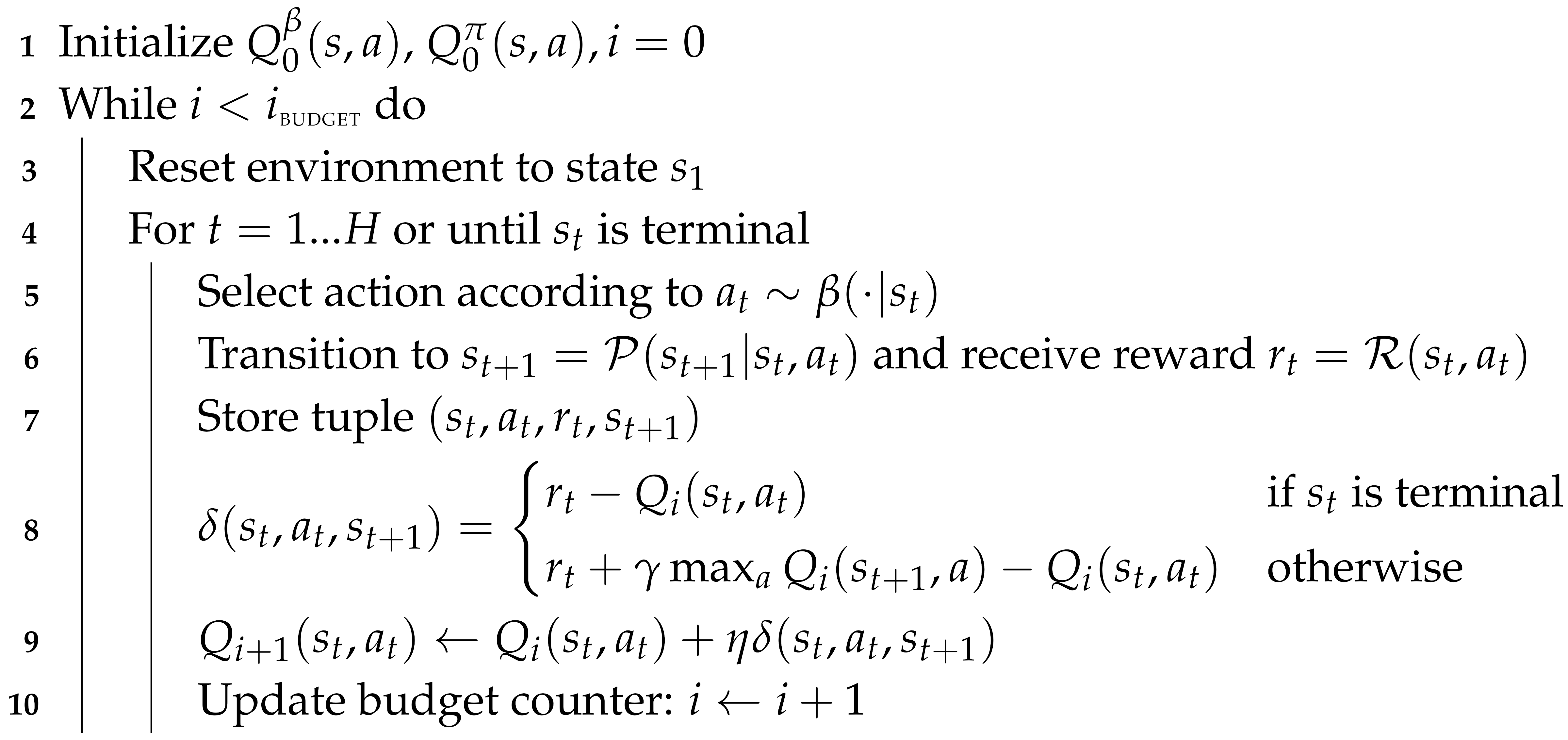
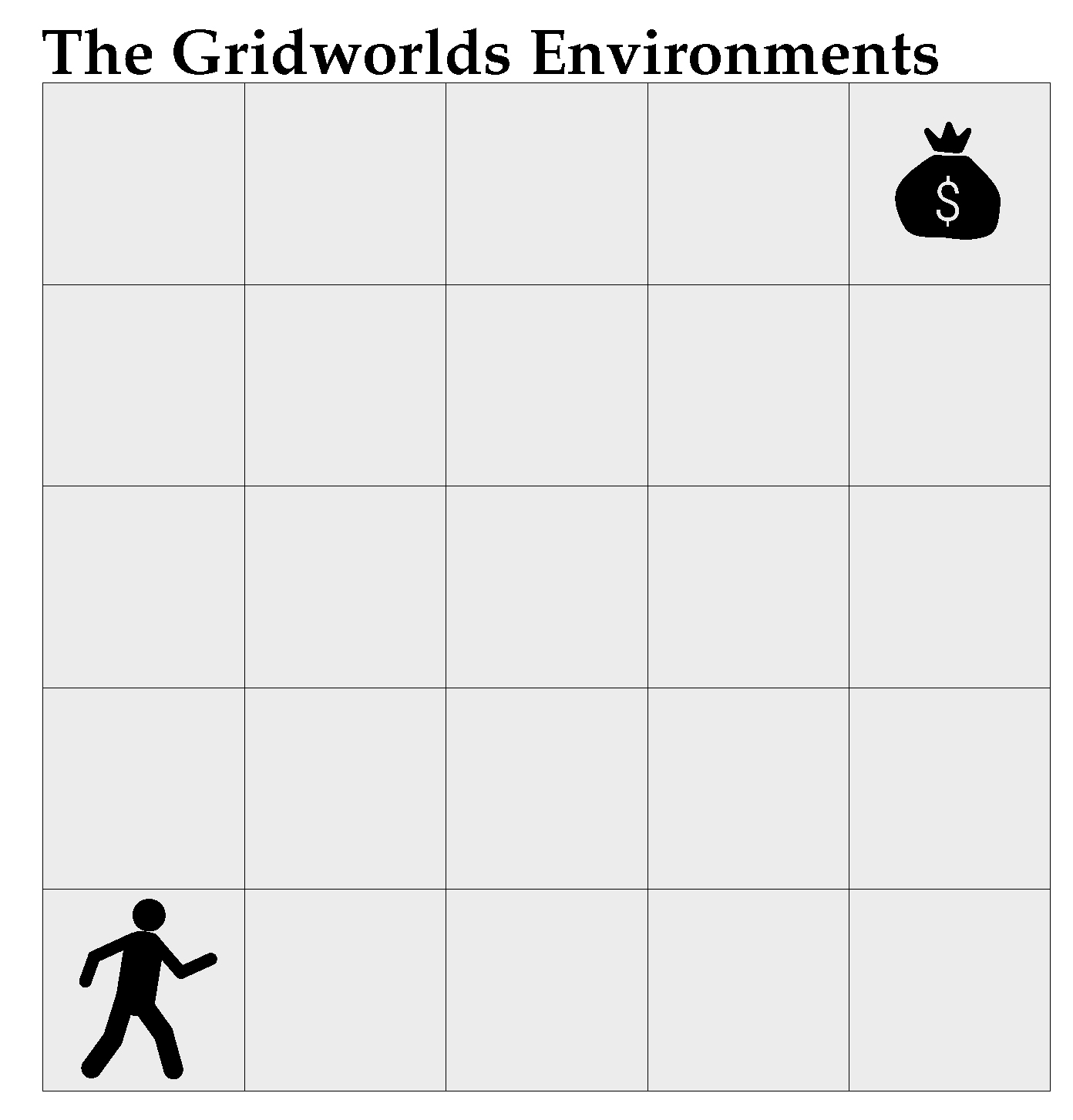
Figure 1.
A simple problem where naive exploration performs poorly. The agent starts in the second leftmost cell and is rewarded only for finding a treasure. It can move up/down/left/right, but if it moves up or down its position resets. Acting randomly at each step takes on average attempts to find the rightmost and most valuable reward, where N is the number of cells to the right of the agent. As no reward is given in any intermediate cell, -greedy exploration is likely to converge to the local optimum represented by the leftmost reward if decays too quickly.
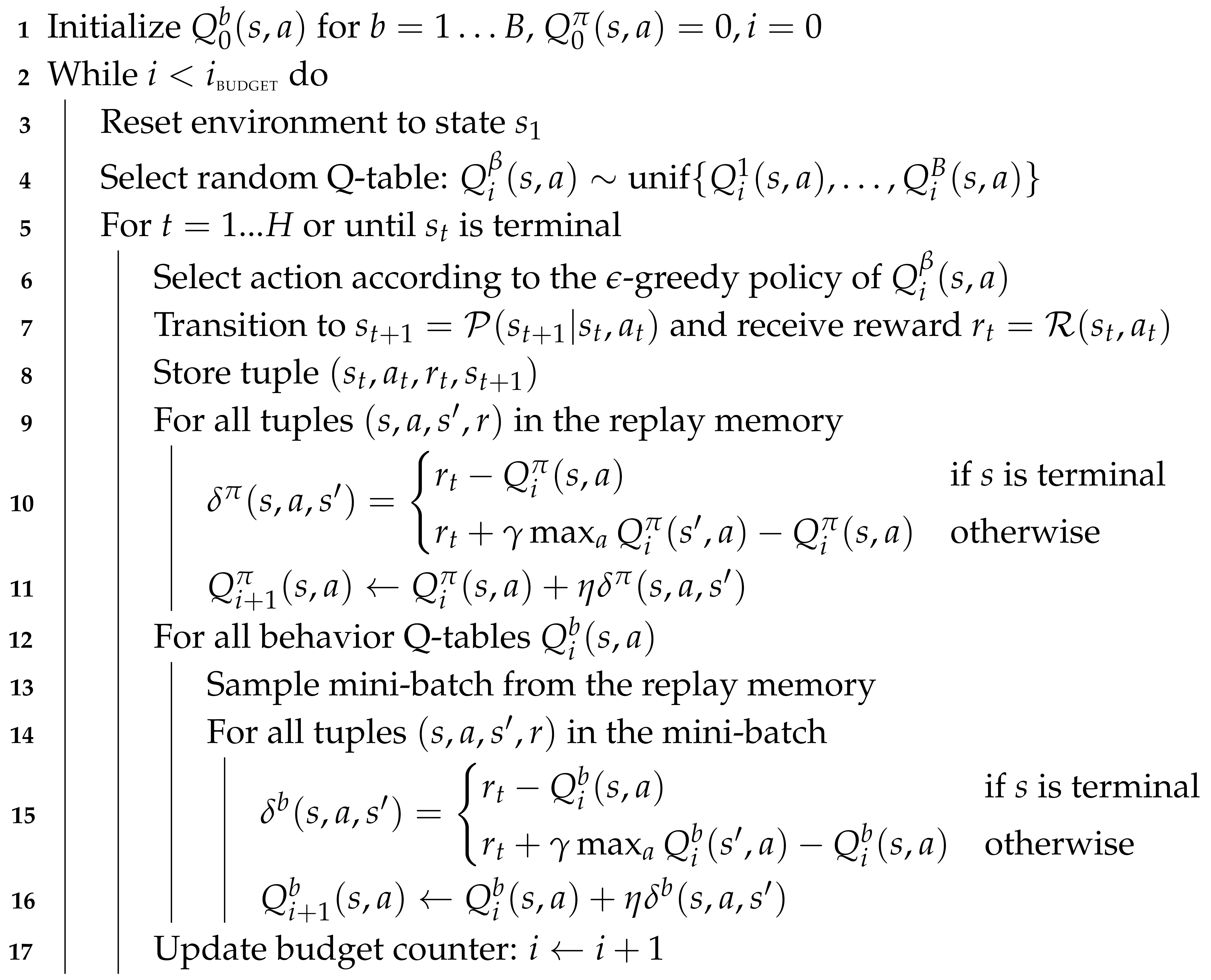
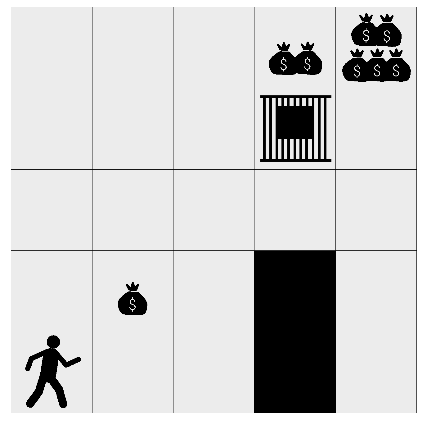
Figure 2.
Toy problem domain.
Figure 2.
Toy problem domain.
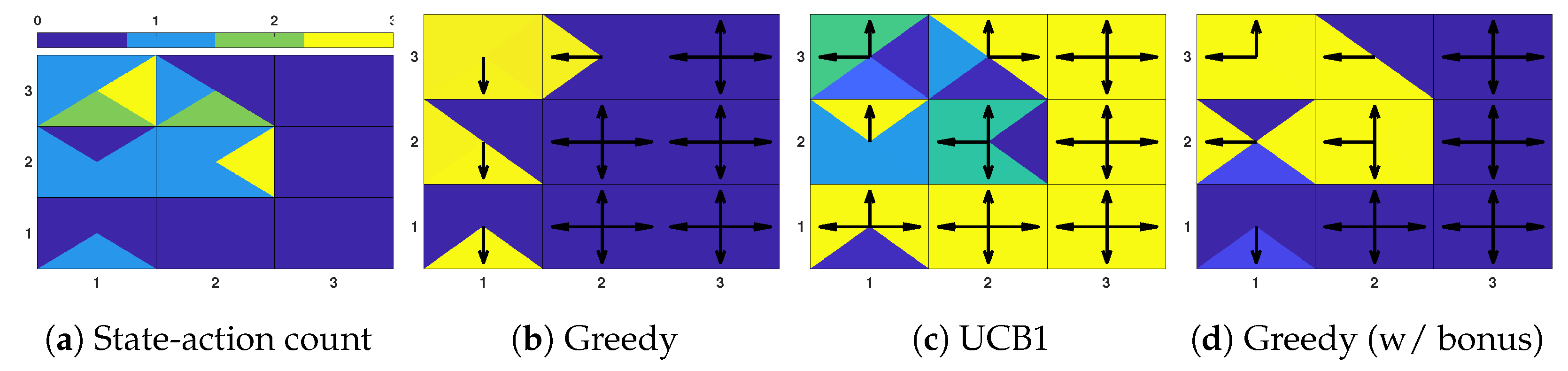
Figure 3.
Toy example (part 1). Visitation count (a) and behavior policies (b–d) for the toy problem below. Cells are divided into four triangles, each one representing the count (a) or the behavior Q-value (b–d) for the actions “up/down/left/right” in that cell. Arrows denote the action with the highest Q-value. None of the behavior policies exhibits long-term deep exploration. In (1,3) both UCB1 (c) and the augmented Q-table (d) myopically select the action with the smallest immediate count. The latter also acts badly in (1,2) and (2,3). There, it selects “left” which has count one, instead of “up” which has count zero.
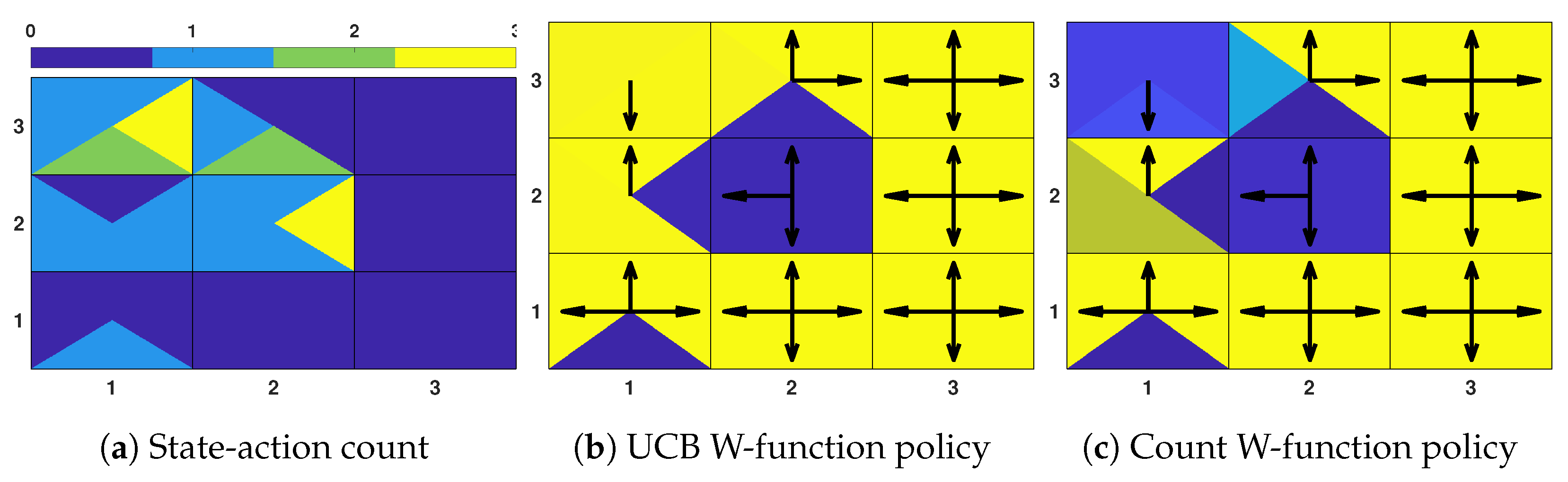
Figure 4.
Toy example (part 2). Visitation count (a) and behavior policies derived from the proposed W-functions (b,c). Due to the low count, the exploration upper bound dominates the greedy Q-value, and the proposed behavior policies successfully achieve long-term exploration. Both policies prioritize unexecuted actions and avoid terminal and prison states.
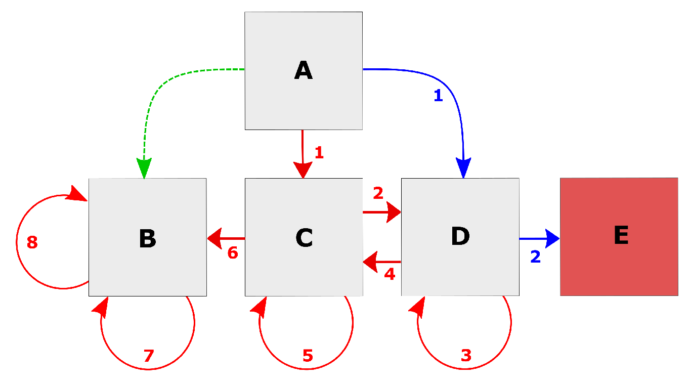
Figure 5.
Chainworld with uniform count.
Figure 5.
Chainworld with uniform count.
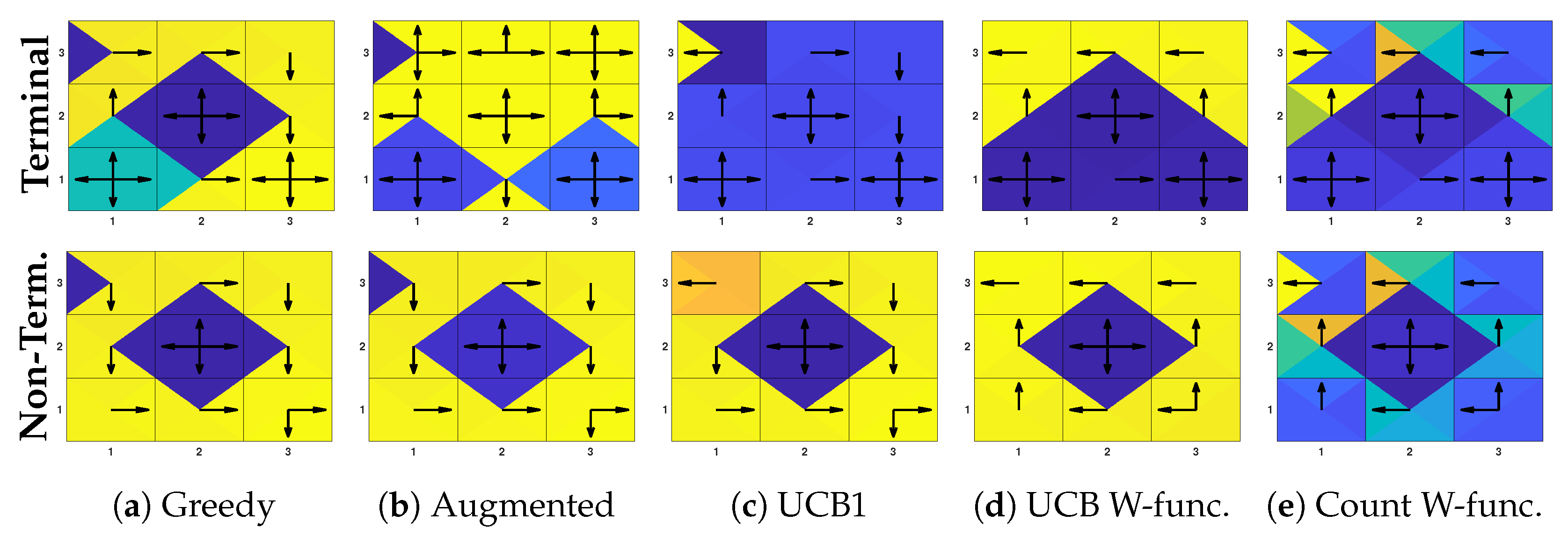
Figure 6.
Toy example (part 3). Behavior policies under uniform visitation count. In the top row, reward states (1,1) and (3,1) are terminal. In the bottom row, they are not and the MDP has an infinite horizon. All state-action pairs have been executed once, except for “left” in (1,3). Only the proposed methods (d,e) correctly identify such state-action pair as the most interesting for exploration and propagate this information to other states thanks to TD learning. When the action is executed, all policies converge to the greedy one (a).
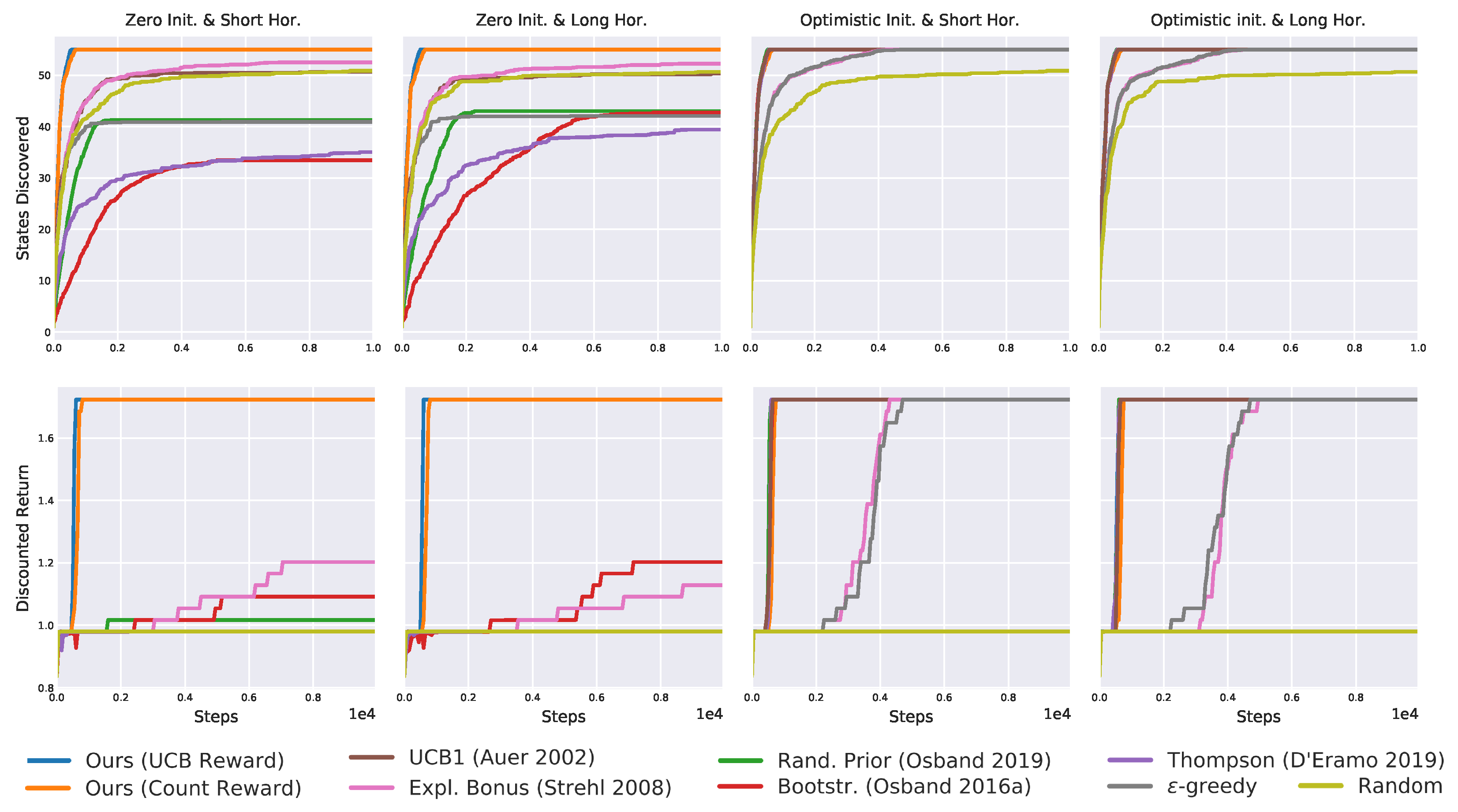
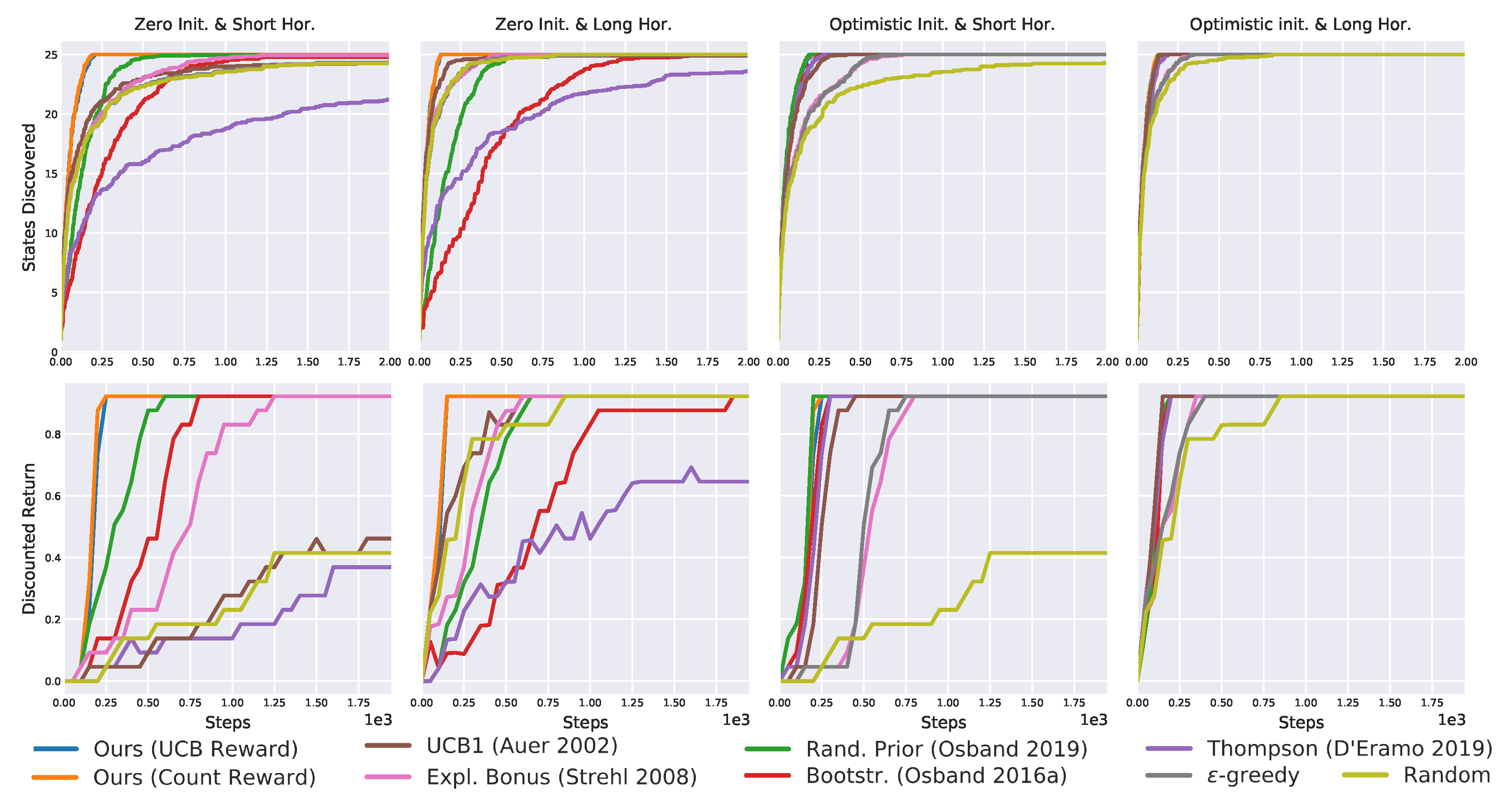
Figure 8.
Results on the deep sea domain averaged over 20 seeds. The proposed exploration achieves the best results, followed by bootstrapped exploration.
Figure 8.
Results on the deep sea domain averaged over 20 seeds. The proposed exploration achieves the best results, followed by bootstrapped exploration.
Figure 9.
The taxi driver.
Figure 9.
The taxi driver.
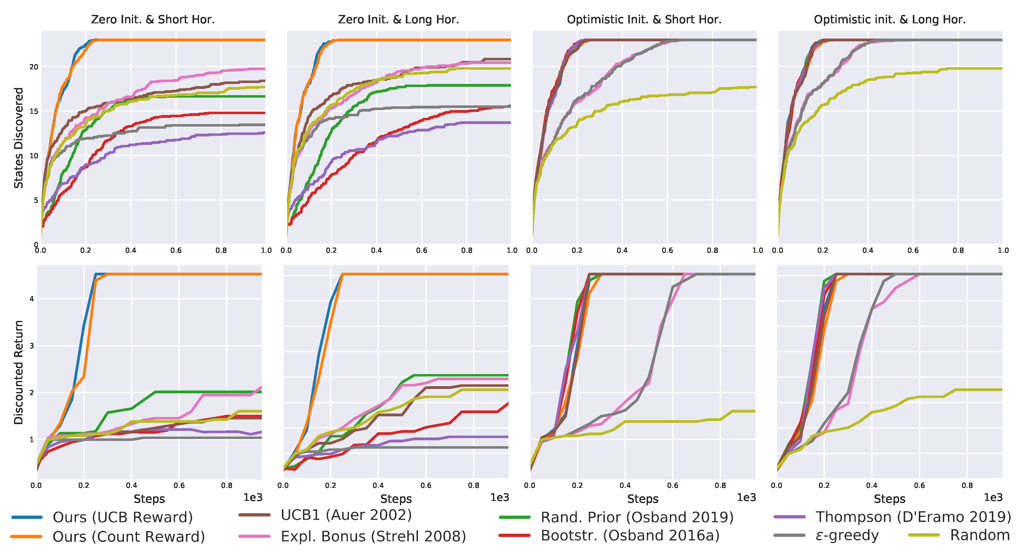
Figure 10.
Results on the taxi domain averaged over 20 seeds. The proposed algorithms outperform all others, being the only solving the task without optimistic initialization.
Figure 10.
Results on the taxi domain averaged over 20 seeds. The proposed algorithms outperform all others, being the only solving the task without optimistic initialization.
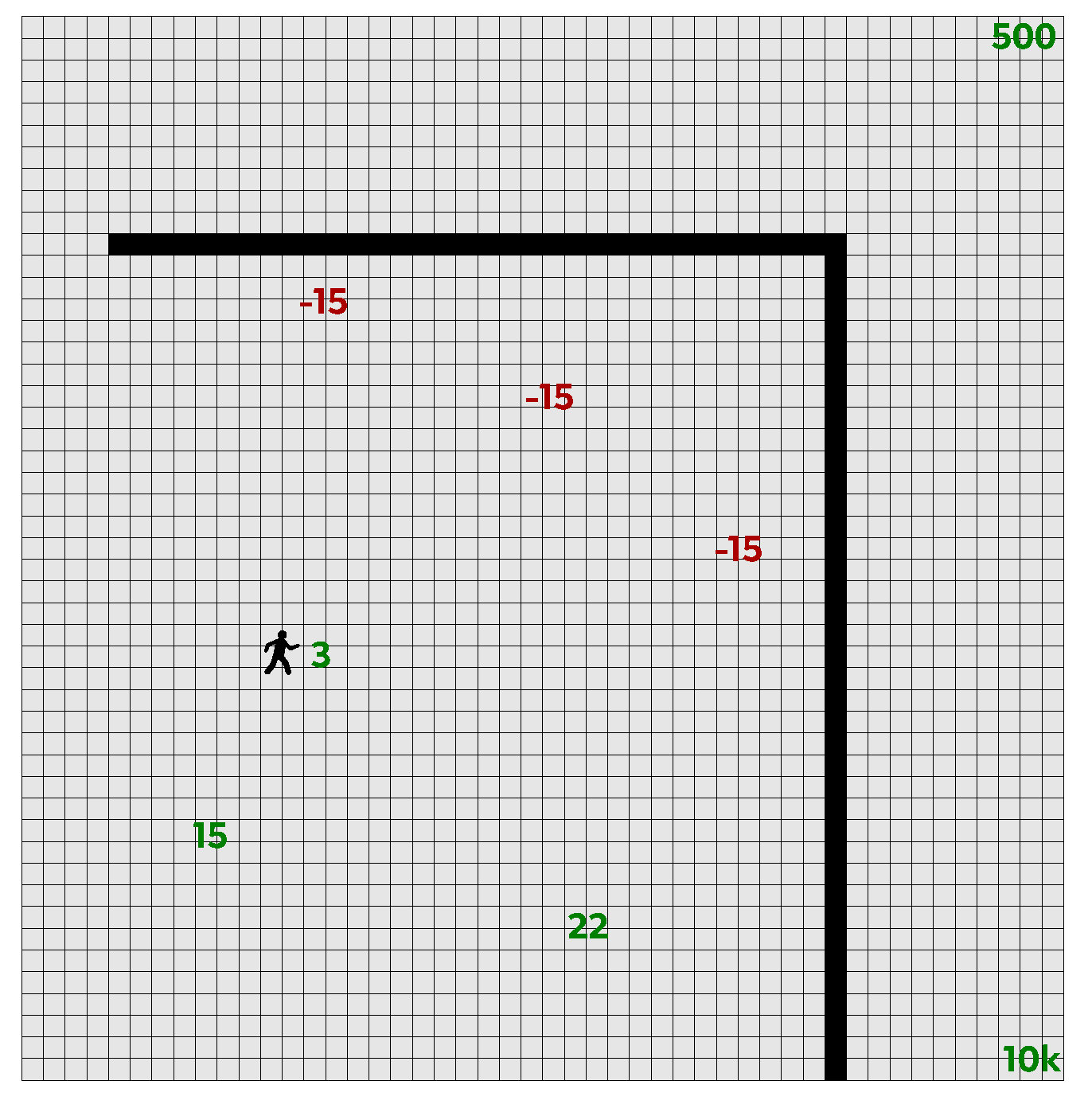
Figure 11.
The deep gridworld.
Figure 11.
The deep gridworld.
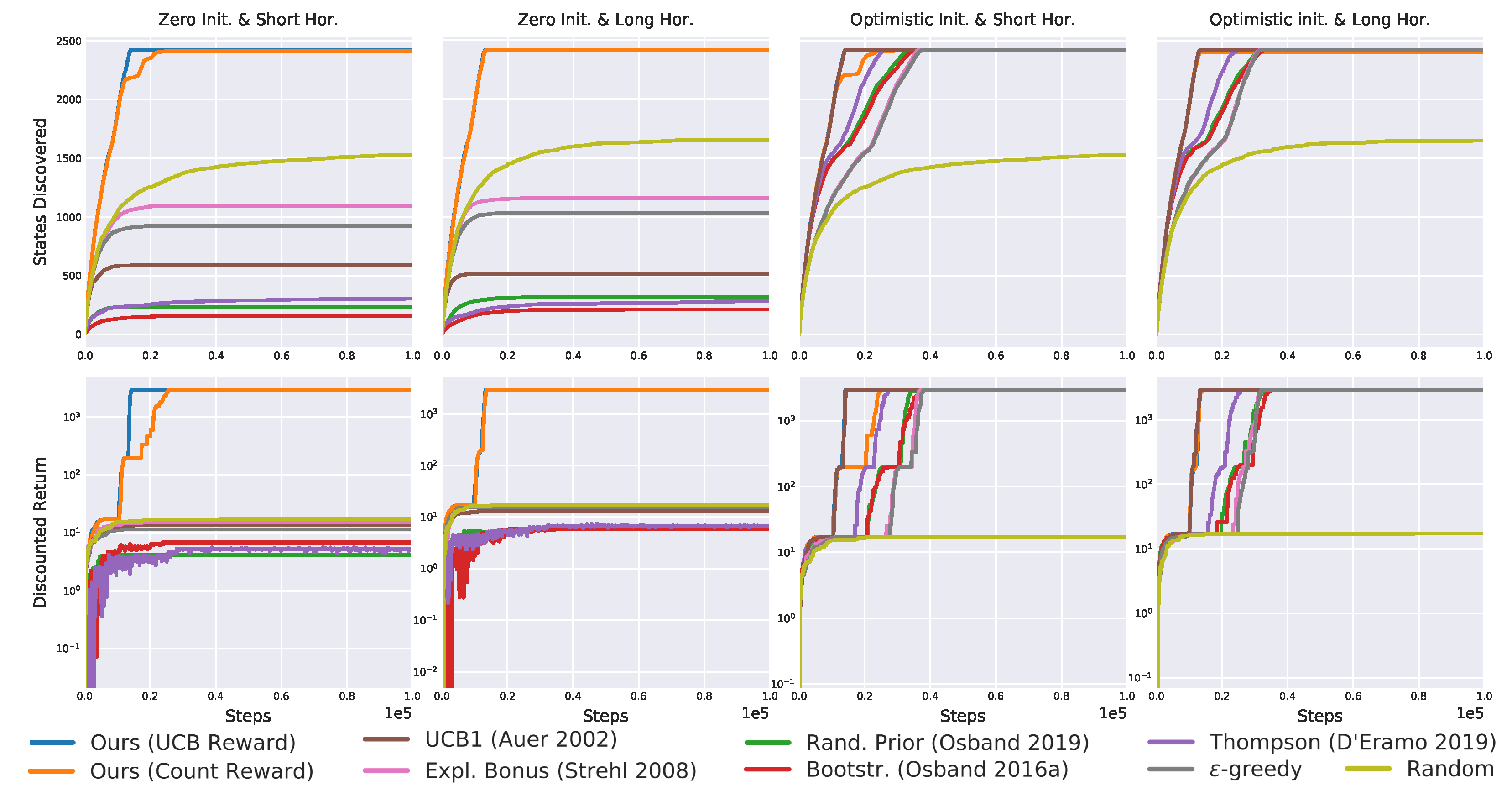
Figure 12.
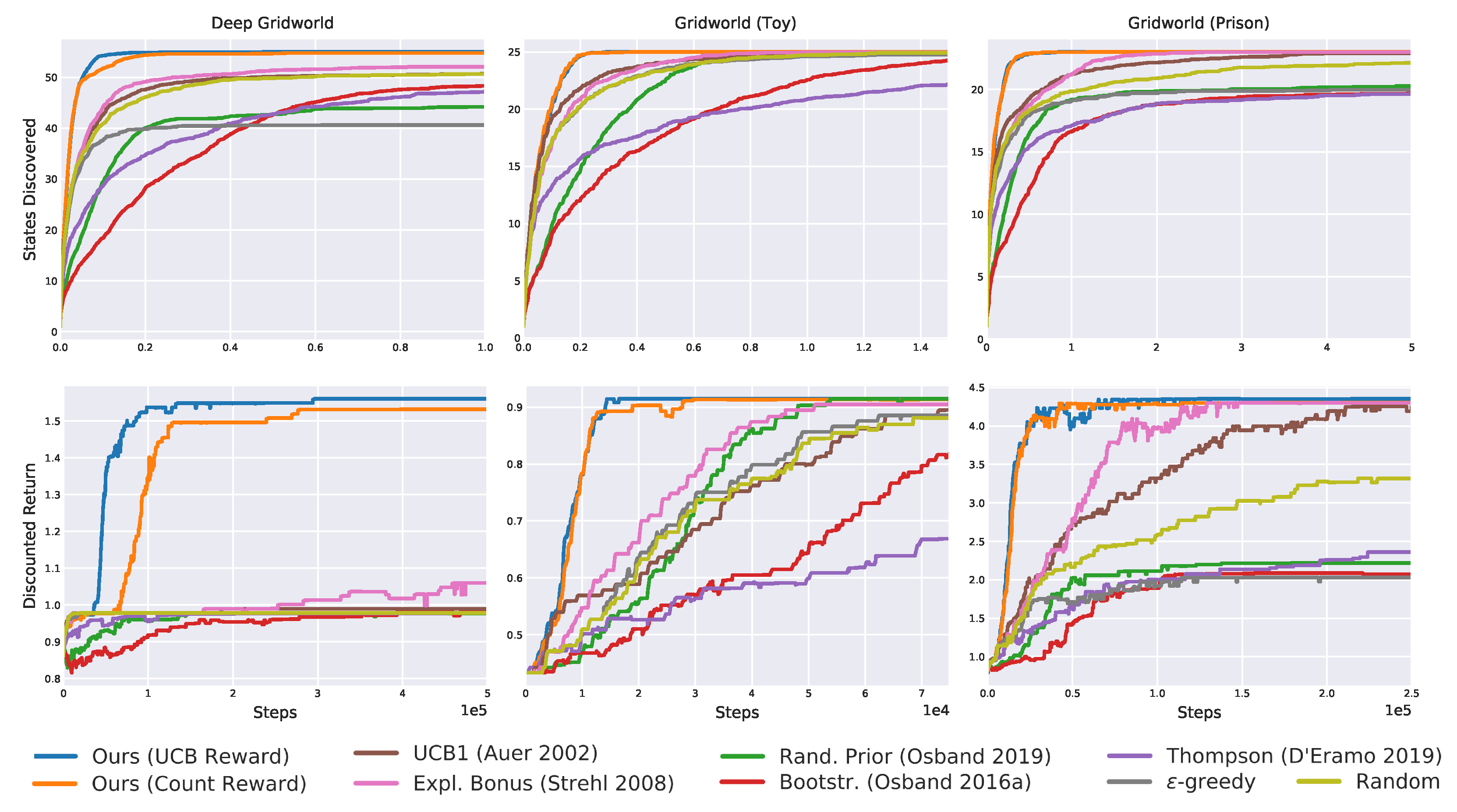
Results on the deep gridworld averaged over 20 seeds. Once again, the proposed algorithms are the only solving the task without optimistic initialization.
Figure 12.
Results on the deep gridworld averaged over 20 seeds. Once again, the proposed algorithms are the only solving the task without optimistic initialization.
Figure 13.
The “toy” gridworld.
Figure 13.
The “toy” gridworld.
Figure 14.
The “prison” gridworld.
Figure 14.
The “prison” gridworld.
Figure 15.
The “wall” gridworld.
Figure 15.
The “wall” gridworld.
Figure 16.
Results on the toy gridworld averaged over 20 seeds. Bootstrapped and bonus-based exploration perform well, but cannot match the proposed one (blue and orange line overlap).
Figure 16.
Results on the toy gridworld averaged over 20 seeds. Bootstrapped and bonus-based exploration perform well, but cannot match the proposed one (blue and orange line overlap).
Figure 17.
The “prison” and distractors affect the performance of all algorithms but ours.
Figure 17.
The “prison” and distractors affect the performance of all algorithms but ours.
Figure 18.
The final gridworld emphasizes the better performance of our algorithms.
Figure 18.
The final gridworld emphasizes the better performance of our algorithms.
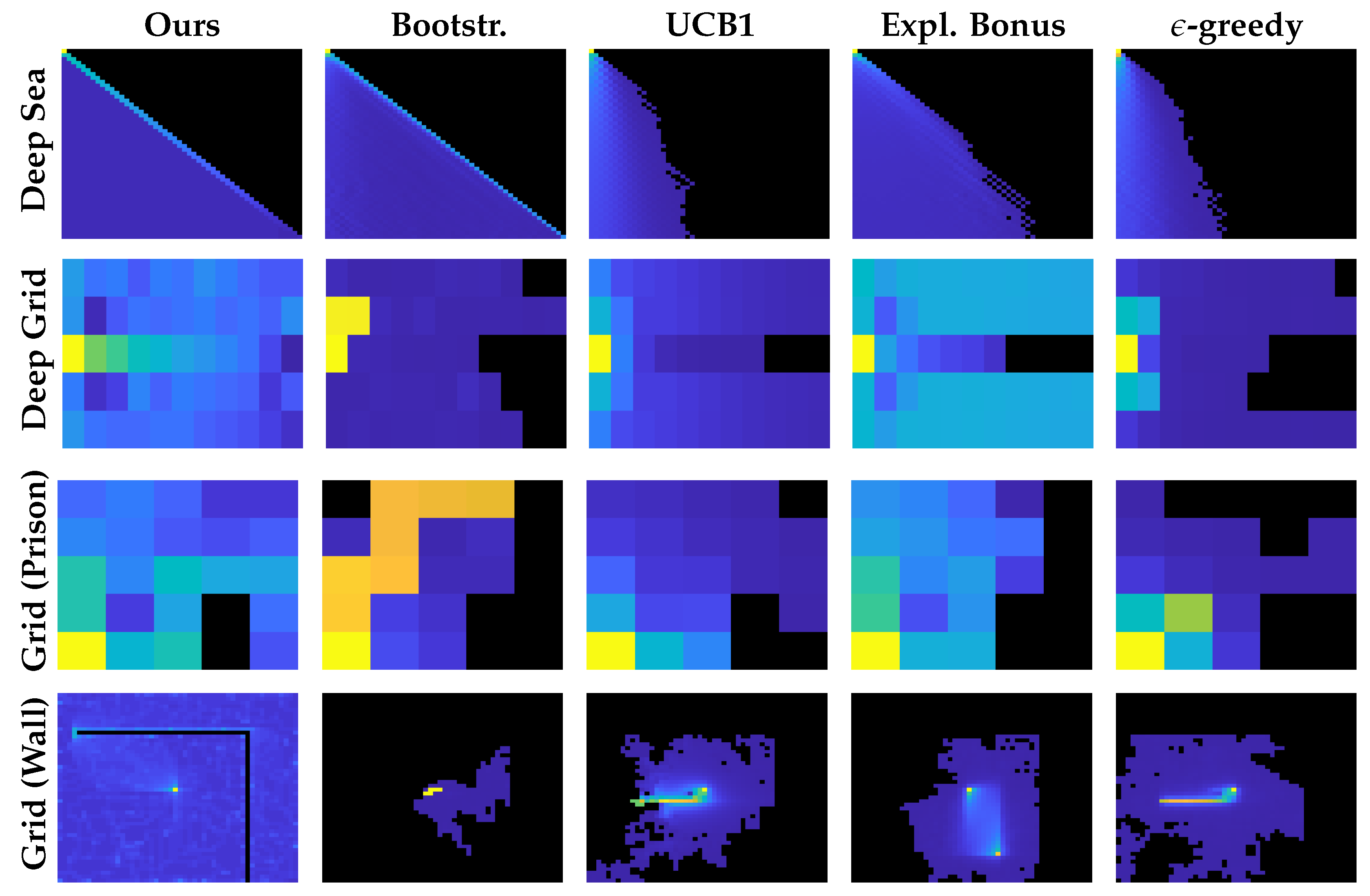
Figure 19.
Visitation count at the end of the learning. The seed is the same across all images. Initial states naturally have a higher count than other states. Recall that the upper portion of the deep sea and some gridworlds cells cannot be visited. Only the proposed methods explore the environment uniformly (figures show the count of UCB-based W-function. Count-based W-function performed very similarly). Other algorithms myopically focus on distractors.
Figure 20.
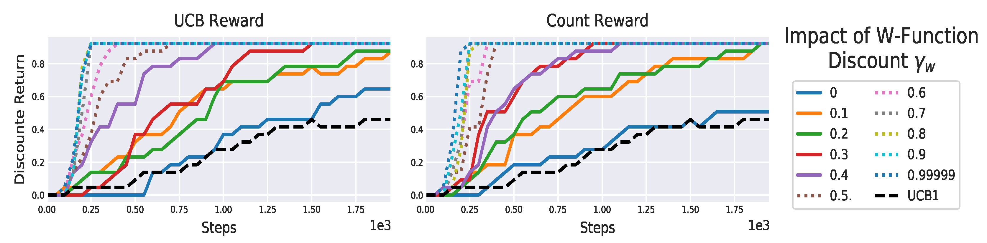
Performance of the our algorithms on varying of on the “toy” gridworld (
Figure 14). The higher
, the more the agent explores, allowing to discover the reward faster.
Figure 20.
Performance of the our algorithms on varying of on the “toy” gridworld (
Figure 14). The higher
, the more the agent explores, allowing to discover the reward faster.
Figure 21.
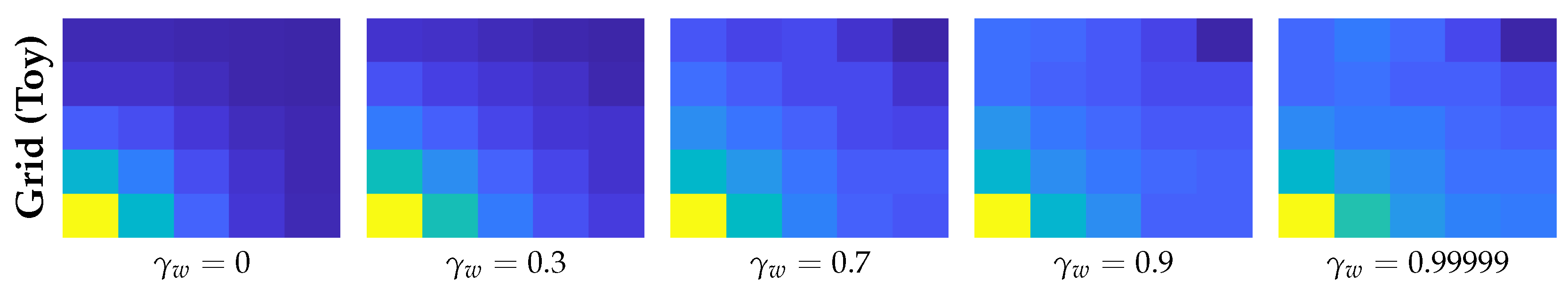
Visitation count forat the end of the learning on the same random seed (out of 20). The higher the discount, the more uniform the count is. The initial state (bottom left) has naturally higher counts because the agent always starts there. performed very similarly.
Figure 21.
Visitation count forat the end of the learning on the same random seed (out of 20). The higher the discount, the more uniform the count is. The initial state (bottom left) has naturally higher counts because the agent always starts there. performed very similarly.
Figure 22.
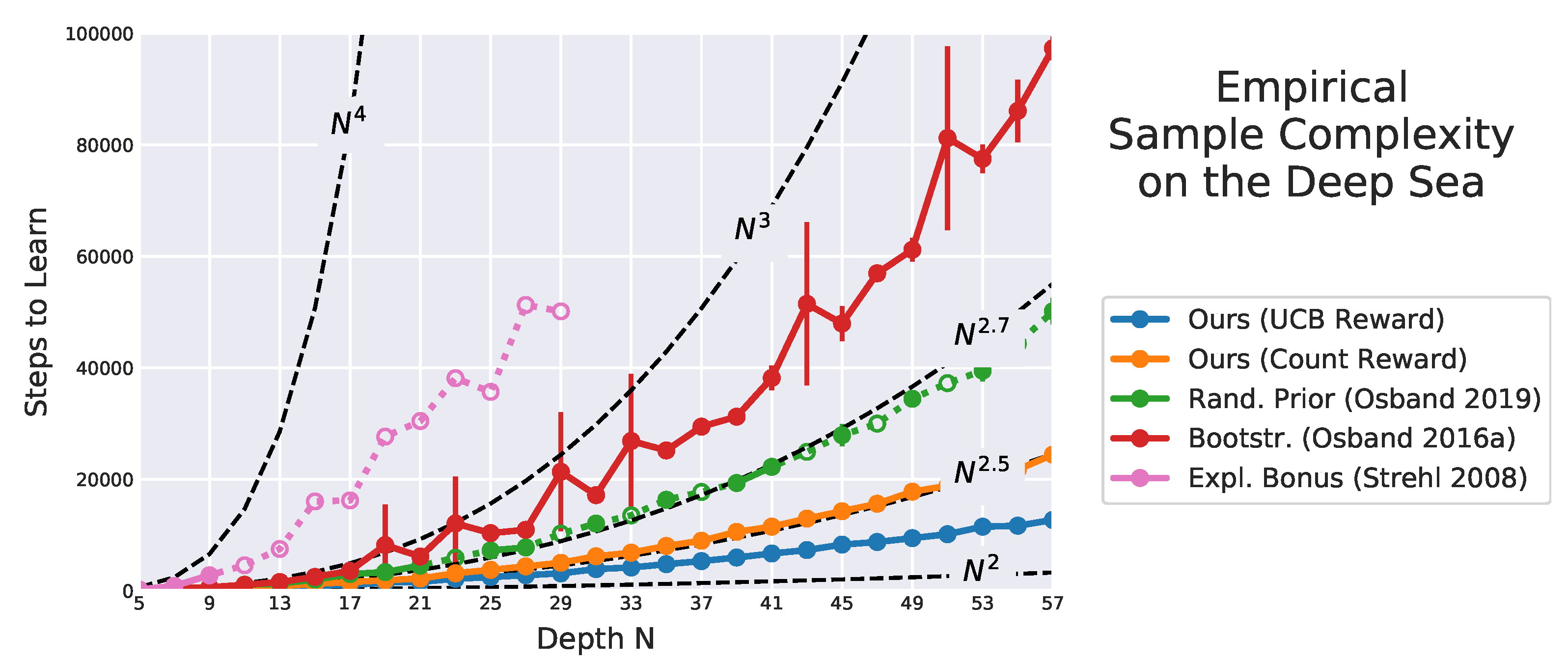
Steps to learn on varying the deep sea size, averaged over ten runs with 500,000 steps limit. For filled dots, the run always converged, and we report the 95% confidence interval with error bars. For empty dots connected with dashed lines, the algorithm did not learn within the step limit at least once. In this case, the average is over converged runs only and we do not report any confidence interval. Using the exploration bonus (pink) learning barely converged once (most of its dots are either missing or empty). Using bootstrapping (red) all runs converged, but the results show a large confidence interval. With random prior (green) the learning rarely did not converge, and performed very similarly across the random seeds, as shown by its extremely small confidence interval. On the contrary, our method (blue, orange) is the only always converging with a confidence interval close to zero. Indeed, it outperforms all baseline by attaining the lowest sample complexity. Missing algorithms (random, -greedy, UCB1, Thompson sampling) performed poorly and are not reported.
Figure 22.
Steps to learn on varying the deep sea size, averaged over ten runs with 500,000 steps limit. For filled dots, the run always converged, and we report the 95% confidence interval with error bars. For empty dots connected with dashed lines, the algorithm did not learn within the step limit at least once. In this case, the average is over converged runs only and we do not report any confidence interval. Using the exploration bonus (pink) learning barely converged once (most of its dots are either missing or empty). Using bootstrapping (red) all runs converged, but the results show a large confidence interval. With random prior (green) the learning rarely did not converge, and performed very similarly across the random seeds, as shown by its extremely small confidence interval. On the contrary, our method (blue, orange) is the only always converging with a confidence interval close to zero. Indeed, it outperforms all baseline by attaining the lowest sample complexity. Missing algorithms (random, -greedy, UCB1, Thompson sampling) performed poorly and are not reported.
![Algorithms 15 00081 g022]()
Figure 23.
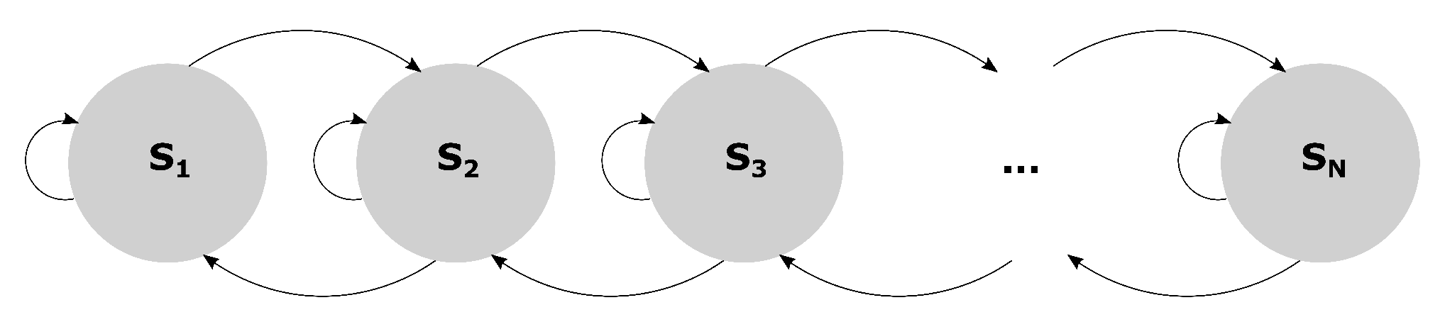
The ergodic chainworld.
Figure 23.
The ergodic chainworld.
Figure 24.
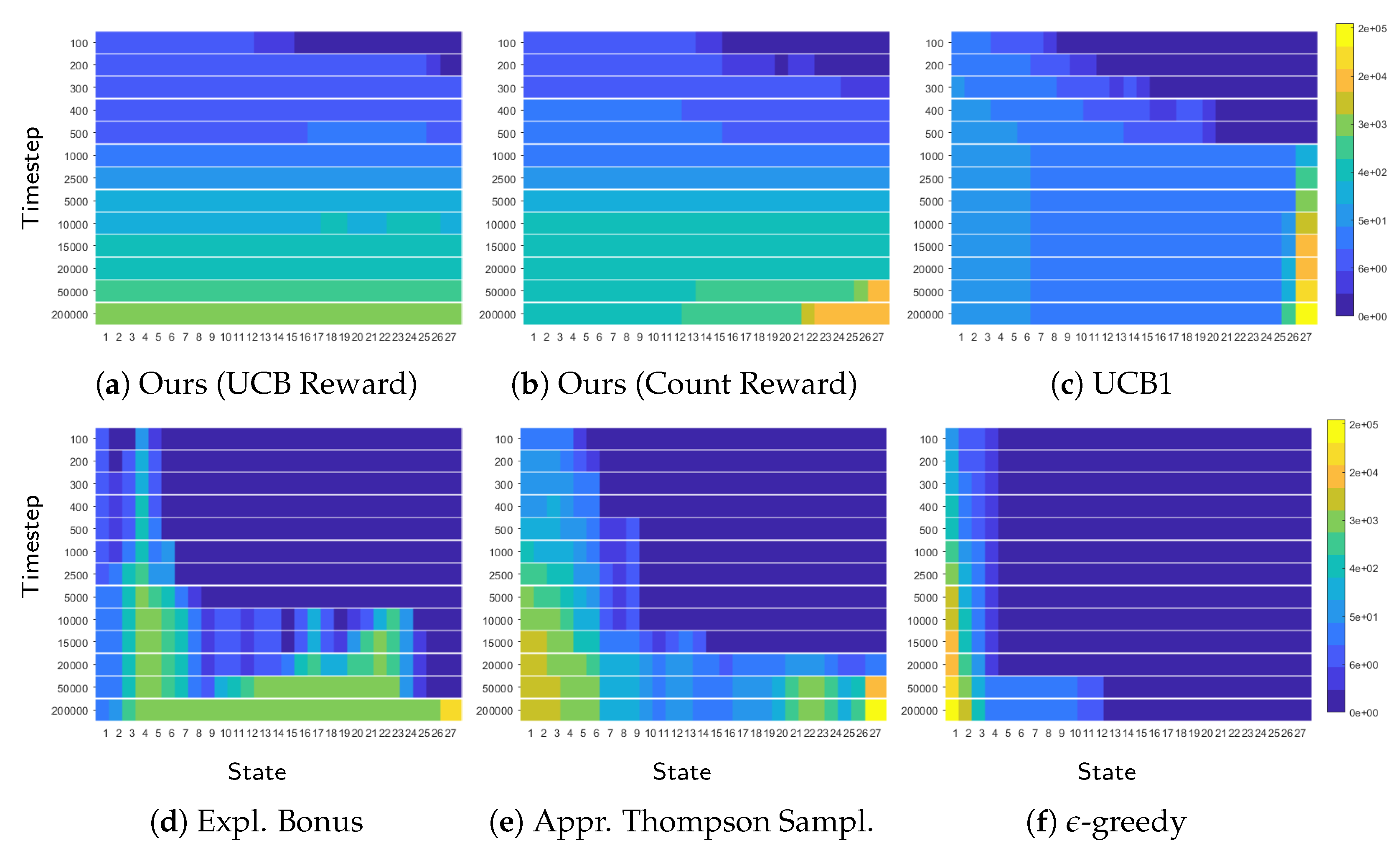
Visitation counts for the chainworld with 27 states (x-axis) over time (y-axis). As time passes (top to bottom), the visitation count grows. Only our algorithms and UCB1 explore uniformly, producing a uniform colormap. However, UCB1 finds the last state (with the reward) much later. Once UCB1 finds the reward ((c), step 1000) the visitation count increases only in the last state. This suggests that when UCB1 finds the reward contained in the last state it effectively stops exploring other states. By contrast, our algorithms keep exploring the environment for longer. This allows the agent to learn the true Q-function for all states and explains why our algorithms achieve lower sample complexity and MSVE.
Figure 24.
Visitation counts for the chainworld with 27 states (x-axis) over time (y-axis). As time passes (top to bottom), the visitation count grows. Only our algorithms and UCB1 explore uniformly, producing a uniform colormap. However, UCB1 finds the last state (with the reward) much later. Once UCB1 finds the reward ((c), step 1000) the visitation count increases only in the last state. This suggests that when UCB1 finds the reward contained in the last state it effectively stops exploring other states. By contrast, our algorithms keep exploring the environment for longer. This allows the agent to learn the true Q-function for all states and explains why our algorithms achieve lower sample complexity and MSVE.
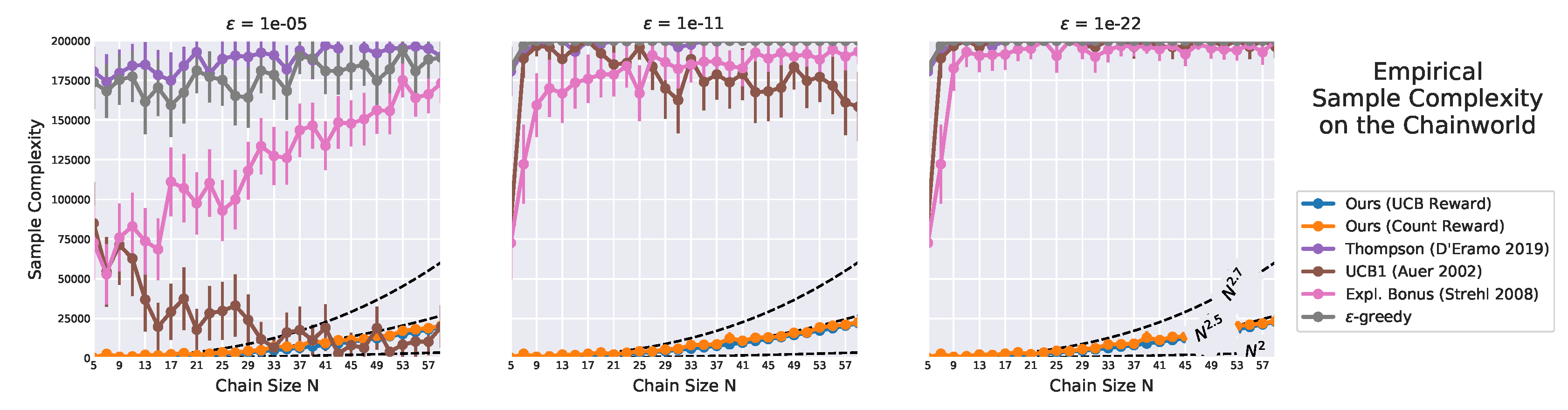
Figure 25.
Sample complexity on varying the chain size. Error bars denote 95% confidence interval. Only the proposed algorithms (blue and orange lines almost overlap) show little sensitivity to , as their sample complexity only slightly increases as decreases. By contrast, other algorithms are highly influenced by . Their estimate complexity has a large confidence interval, and for smaller they rarely learn an -optimal policy.
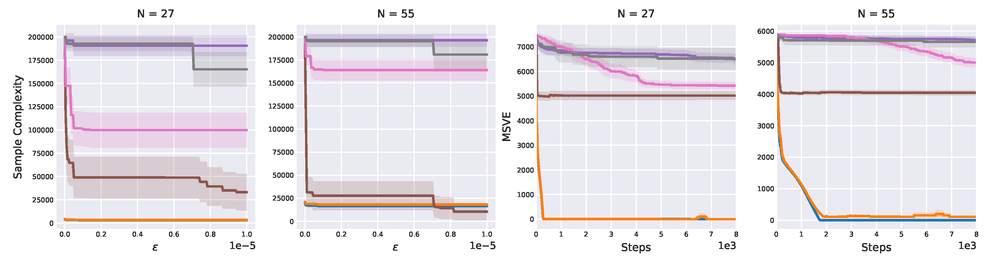
Figure 26.
Sample complexity against , and MSVE over time for 27- and 55-state chainworlds. Shaded areas denote 95% confidence interval. As shown in
Figure 25, the sample complexity of our approach is barely influenced by
. Even for
, our algorithms attain low sample complexity, whereas other algorithms complexity is several orders of magnitude higher. Similarly, only our algorithms learn an almost perfect Q-function, achieving an MSVE close to zero.
Figure 27.
Results with stochastic transition function on three of the previous MDPs. Once again, only our algorithms visit all states and learn the optimal policy within steps limit in all MDPs, and their performance is barely affected by the stochasticity.
Figure 27.
Results with stochastic transition function on three of the previous MDPs. Once again, only our algorithms visit all states and learn the optimal policy within steps limit in all MDPs, and their performance is barely affected by the stochasticity.
Table 1.
Results recap for the “zero initialization short horizon”. Only the proposed exploration strategy always discovers all states and solves the tasks in all 20 seeds.
Table 1.
Results recap for the “zero initialization short horizon”. Only the proposed exploration strategy always discovers all states and solves the tasks in all 20 seeds.
| | Algorithm | Discovery (%) | Success (%) |
|---|
| | Ours (UCB Reward) | | |
| | Ours (Count Reward) | | |
| | Rand. Prior (Osband 2019) | | |
| | Bootstr. (Osband 2016a) | | |
| Deep Sea | Bootstr. (D’Eramo 2019) | | |
| | UCB1 (Auer 2002) | | |
| | Expl. Bonus (Strehl 2008) | | |
| | -greedy | | |
| | Random | | |
| | Ours (UCB Reward) | | |
| | Ours (Count Reward) | | |
| | Rand. Prior (Osband 2019) | | |
| | Bootstr. (Osband 2016a) | | |
| Taxi | Bootstr. (D’Eramo 2019) | | |
| | UCB1 (Auer 2002) | | |
| | Expl. Bonus (Strehl 2008) | | |
| | -greedy | | |
| | Random | | |
| | Ours (UCB Reward) | | |
| | Ours (Count Reward) | | |
| | Rand. Prior (Osband 2019) | | |
| | Bootstr. (Osband 2016a) | | |
| Deep Gridworld | Bootstr. (D’Eramo 2019) | | |
| | UCB1 (Auer 2002) | | |
| | Expl. Bonus (Strehl 2008) | | |
| | -greedy | | |
| | Random | | |
| | Ours (UCB Reward) | | |
| | Ours (Count Reward) | | |
| | Rand. Prior (Osband 2019) | | |
| | Bootstr. (Osband 2016a) | | |
| Gridworld (Toy) | Bootstr. (D’Eramo 2019) | | |
| | UCB1 (Auer 2002) | | |
| | Expl. Bonus (Strehl 2008) | | |
| | -greedy | | |
| | Random | | |
| | Ours (UCB Reward) | | |
| | Ours (Count Reward) | | |
| | Rand. Prior (Osband 2019) | | |
| | Bootstr. (Osband 2016a) | | |
| Gridworld (Prison) | Bootstr. (D’Eramo 2019) | | |
| | UCB1 (Auer 2002) | | |
| | Expl. Bonus (Strehl 2008) | | |
| | -greedy | | |
| | Random | | |
| | Ours (UCB Reward) | | |
| | Ours (Count Reward) | | |
| | Rand. Prior (Osband 2019) | | |
| | Bootstr. (Osband 2016a) | | |
| Gridworld (Wall) | Bootstr. (D’Eramo 2019) | | |
| | UCB1 (Auer 2002) | | |
| | Expl. Bonus (Strehl 2008) | | |
| | -greedy | | |
| | Random | | |


 ,
, 
