An Effective Algorithm for Finding Shortest Paths in Tubular Spaces

Abstract

We propose a novel algorithm to determine the Euclidean shortest path (ESP) from a given point (source) to another point (destination) inside a tubular space. The method is based on the observation data of a virtual particle (VP) assumed to move along this path. In the first step, the geometric properties of the shortest path inside the considered space are presented and proven. Utilizing these properties, the desired ESP can be segmented into three partitions depending on the visibility of the VP. Our algorithm will check which partition the VP belongs to and calculate the correct direction of its movement, and thus the shortest path will be traced. The proposed method is then compared to Dijkstra’s algorithm, considering different types of tubular spaces. In all cases, the solution provided by the proposed algorithm is smoother, shorter, and has a higher accuracy with a faster calculation speed than that obtained by Dijkstra’s method.

1. Introduction

Finding the shortest path in the presence of obstacles, referred to as the Euclidean shortest path problem, is one of the fundamental problems in path planning [1]. This problem arises in many industrial applications. The idea of using a flying robot such as an unmanned aerial vehicle (UAV) to navigate through a tunnel-like environment can be found in the inspection of dam penstocks [2,3,4], chimneys [5], ventilation systems [6], onshore oil and gas industry [7], narrow sewers [8], and other hazardous deep tunnels [9,10]. In addition, many marine applications also require navigating through underwater tunnel-like environments with autonomous underwater vehicles (AUVs). These include, for instance, the inspection of different kinds of underwater structures such as offshore oil platforms [11], flooded spring tunnels [12,13], water delivery tunnels [14], etc. In these applications, shortest path planning that minimizes the total distance travelled by the vehicles plays an important role in optimizing the energy consumption, thus extending the operation time without recharging their batteries [15,16]. It may also reduce the travelling time and will be very useful for search and rescue missions during disaster events in underground tunnels [6,17].

Another example of the studied problem is to determine the location of a non-elastic chord between two points within a tube. Indeed, this problem can be found in controlling the deformation of slender tube-like robots actuated with at least one internal tendon [18,19]. Calculating the tendon load effect on the tube wall requires determining the tendon location. As it is only attached at the tip, pre-positioned at the base, and the rest freely locates inside the innermost tube, its location results in the shortest path connecting two points at the base and at the tip.

1.1. Related Works

In general 3D space, the problem of finding the ESP between two given points that does not intersect with any given obstacles is known to be NP-hard [20]: special cases of this problem have been studied as follows. The authors in [21] gave a polynomial time algorithm to calculate ESP for cases in which the number of obstacles is ‘small’ and all of them are convex. Another algorithm was proposed in [22] with the assumption that all obstacles are vertical buildings with k different heights. More recently, Ref. [23] presented algorithms for solving approximate ESPs amid convex obstacles. Other approximation algorithms for ESP calculations are detailed in [24]. These studies share common features in that a collection of finite obstacles are given as forbidden zones in space and the ESP will be found in the space surrounding these obstacles.

In the studied problem, the obstacle is the entire space outside the tube and the ESP must pass through the inner zone of the tubular space. A similar problem can be found in [25] that computes the minimal path in tubular space. The minimal path is typically solved based on the Fast Marching Method (FMM) which only considers grid nodes as the possible vertices of the minimal paths. However, the paths detected by the FMM have been proven to be not always the exact ESPs [1]. Several approximation algorithms also exist for finding the ESP between two points in 3D space bounded by a closed surface such as cube-curves [26] or a simple polyhedron [27] using the rubberband algorithm. This method is suitable for solving various ESPs in 3D space. Even so, there is a non-trivial gap in the geometric shape between the cube-curve and the tubular space. Polyhedron seems like a better choice to represent a tubular space. However, the characteristic geometrical properties of tubular spaces should be considered for a dedicated algorithm.

The study of a tubular surface with Bishop frame was proposed in [28]. The authors provided some characterizations about the special curves lying on this surface (e.g., geodesic and asymptotic curves). However, the problem studied herein requires considering the interior space instead of just the boundary surface. In addition, the geometrical properties of the ESP inside the tubular space also need to be investigated. The authors in [29] described a simple geometric structure of ESPs where they consist of curved paths on the obstacles connected by straight line segments (see Theorem 1). In this work, we develop the geometric structure of ESPs presented in [29] by considering the characteristic properties of tubular spaces.

In practice, the navigation problem can be classified into planning-based and reactive algorithms [30]. Planning-based approaches require a global map representation of the environment (e.g., a graph or a network) before searching. Prior knowledge of the tubular space enables the generation of a weighted graph where the weight of each edge (or arc for the directed graph) is associated with its length [24]. Numerous algorithms are used for the shortest path calculation in graph theory (see Chapters 24 and 25 in [31]). A well-known graph-based algorithm among them is Dijkstra’s algorithm [32] in which the shortest path connects vertices in the graph. Unlike the planning-based approaches, a reactive method allows directly generating motion decisions during the movement based on observed data [30]. The reactive shortest path navigation was presented in [33] for an in-plane problem. Such a problem was also found in 3D space where the obtained path is interpolated with a spline curve [34]. In this work, we propose an algorithm based on the observed information of a virtual particle that can be used as a reactive method for the shortest path navigation inside the tubular space.

1.2. Contributions

In this paper, we propose a novel algorithm to find the shortest path within a tubular space that connects two points at the tube ends. Our contributions include: (1) the description of the ESP geometrical structure inside tubular spaces with mathematical proof; (2) the proposition of a novel algorithm for finding the shortest path in tubular spaces based on the observed data; and (3) the numerical validation and comparison results with Dijkstra’s algorithm by considering various types of tubular spaces. As a result, the solution obtained by using the proposed algorithm is shorter, smoother and faster than that provided by Dijkstra’s method.

The remainder of this paper is organized as follows. Section 2 formulates the problem. The basics of Dijkstra’s algorithm are described in Section 3. Then, we present the proposed algorithm in Section 4. Our computational results are provided in Section 5. After that, Section 6 includes some brief discussions. Section 7 concludes the paper.

2. ESP in Tubular Space

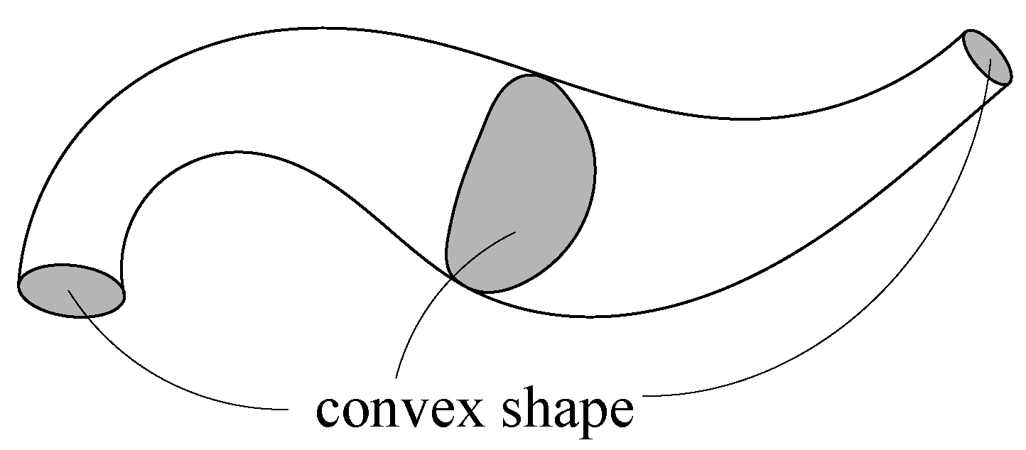
2.1. Problem Description

Euclidean geometry is the geometry in daily life [1] where the distance between two points $\mathit{p}={(x_p,\phantom{.}{y}_p,\phantom{.}{z}_p)}^T$ and $\mathit{q}={(x_q,\phantom{.}{y}_q,\phantom{.}{z}_q)}^T$ in 3D space is defined as follows:

$$d_e(\mathit{p},\phantom{.}\mathit{q})=\sqrt{{(x_p-x_q)}^2+{(y_p-y_q)}^2+{(z_p-z_q)}^2}$$

(1)

From the discrete point of view, a path $\left(\alpha \right)$ from the source $\mathfrak{P}$ to the destination $\mathfrak{Q}$ is a finite sequence of nodes ${\mathit{x}}_i$, starting at $\mathfrak{P}$ and ending at $\mathfrak{Q}$. We obtain the length of the path as in Equation (2):

$$L\left(\alpha \right)=\sum _{i=0}^{n-1}{d}_e({\mathit{x}}_{\mathit{i}},\phantom{.}{\mathit{x}}_{\mathit{i}+\mathit{1}}),{\mathit{x}}_0=\mathfrak{P},\phantom{.}{\mathit{x}}_n=\mathfrak{Q}$$

(2)

Then, the ESP is the path connecting $\mathfrak{P}$ and $\mathfrak{Q}$, which has the minimum length and has to be through a given tubular space. The mathematical definition of tubular space is given as follows [35]:

Definition 1.

Let $\mathit{c}\left(s\right):I\to {\mathbb{R}}^3$ be a smooth, regular space curve. A tubular surface $\partial \mathsf{\Omega }$ associated to $\mathit{c}$(s), of radius ρ, is, by definition, the envelope of the family of spheres of radius ρ, with the center on the curve.

Definition 2.

The storage space of the tube Ω is the 3D space enclosed by the lateral wall ($\partial \mathsf{\Omega }$) and the two ending cross-sections of the tube.

In Definition 1, s is the arc length parameter of the centerline curve. In this work, we consider the tubular surface $\partial \mathsf{\Omega }$ to be regular (Figure 1). The condition underlying the regularity of a tube is given in detail in [28]. By $\kappa \left(s\right)$, we denote the curvature of the centerline curve $\mathit{c}\left(s\right)$. In order to avoid singularities as well as self-overlapping, the following condition is required:

$$\kappa \left(s\right)<{\rho }^{-1},\forall s\in \left[0,L\right]$$

(3)

where L is the length of $\mathit{c}\left(s\right)$.

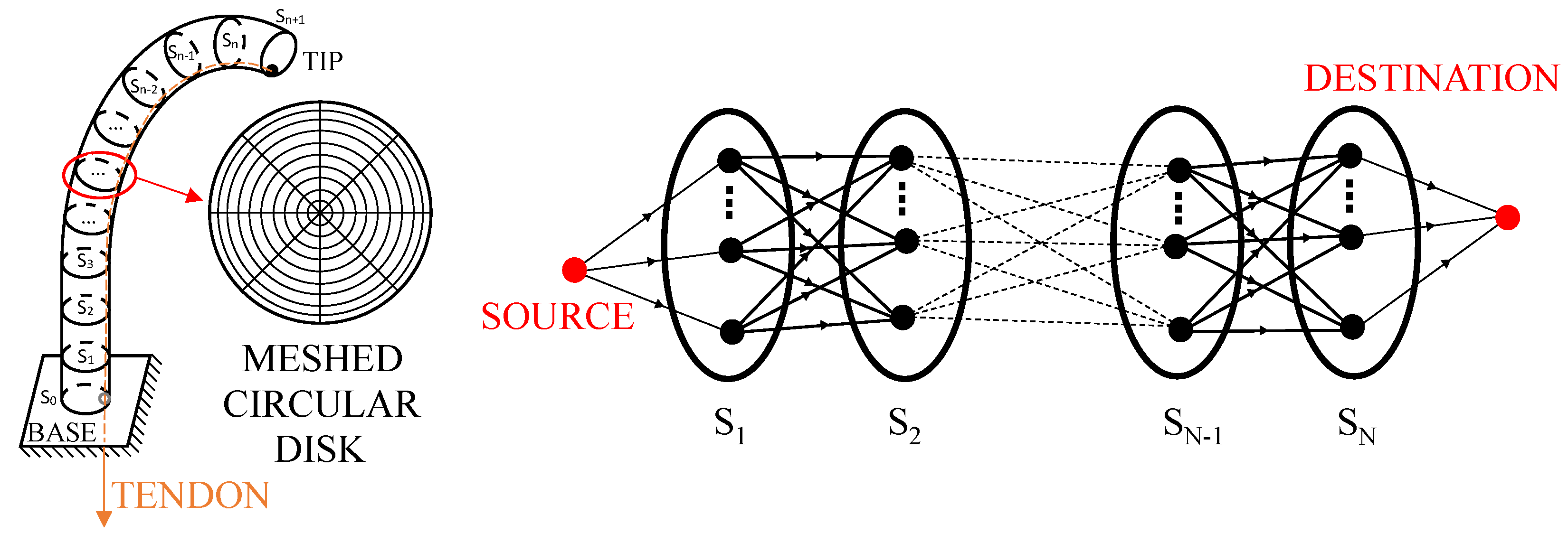
2.2. Directed Graph

We discretize $\mathsf{\Omega }$ into a series of meshed circular disks corresponding to the cross-sections perpendicular to $\mathit{c}\left(s\right)$. By $S_0,\cdots ,S_{N+1}$, we denote the meshed circular disks where $S_0$ contains the starting point (source) $\mathfrak{P}$ and $S_{N+1}$ includes the destination $\mathfrak{Q}$. The distance between two consecutive disks along the centerline curve is $h=\frac{L}{N+1}$. As the shortest path from the source to the destination must obviously pass through each cross-section at only one point, we have the weighted directed graph $G(V,A)$, as shown in Figure 2. This directed graph is defined by a finite set V of vertices and a set A of arcs between those vertices [1]. All vertices of the graph (except $\mathfrak{P}$ and $\mathfrak{Q}$) are located at the nodes of the meshed disks $S_1,\cdots ,S_N$. We define two vertices as adjacent if they are connected by one arc. Then, every two adjacent nodes in the graph are located on two consecutive disks. The source $\mathfrak{P}$ is connected with all nodes of disk $S_1$. Each node of disk $S_i$ is connected by one arc to every node of disk $S_{i+1}$ for all $i\in \{1,\cdots ,N-1\}$. Eventually, every node of disk $S_N$ is directly connected to the destination $\mathfrak{Q}$.

3. Basics of Dijkstra’s Algorithm

The concept of this method, based on the lemma about the relationship between the global minimum and local minimum, was first presented by E.W. Dijkstra in 1959 (see [32], Problem 2). Despite also being based on Lemma 1, if applied to the directed graph, Algorithm 1 has a run time in $O\left(\right|A\left|\right)$ instead of $O\left(\right|V\left|log\right|V|+|A\left|\right)$, as is the case for the conventional Dijkstra’s algorithm used for a weighted graph [1]. In the literature, the $A^{*}$ algorithm [36] is a good method for searching the shortest path in a weighted graph as it improves the calculation speed of Dijkstra’s algorithm for many cases. However, choosing an effective admissible heuristic function for this algorithm based on the geometry of the tubular space is beyond the scope of this paper. In addition, the complexity $O\left(\right|A\left|\right)$ is already a good run time for this problem, so we do not consider the $A^{*}$ algorithm in this work.

Lemma 1

(Dijkstra algorithm, 1959). “If $\mathit{r}$ is a node on the minimal path from $\mathit{p}$ to $\mathit{q}$, the knowledge of the latter implies the knowledge of the minimal path from $\mathit{p}$ to $\mathit{r}$”.

This lemma can easily be proven by contradiction. The shortest path from the source $\mathfrak{P}$ to the destination $\mathfrak{Q}$ will be traced by extending all extendable paths by one edge to a node not yet visited on this path until $\mathfrak{Q}$ is reached. Consequently, extending all the extendable paths from the source by one arc in the directed graph starts to turn the examined disk into its adjacent disk towards the destination. Upon examining a disk, the shortest path between the source and every node on the previous disks has been identified, so we do not need to revisit these points.

Set ${\mathit{r}}_{\left[i\right]\left[j\right]}(i\in \{1,\cdots ,N\},j\in \{1,\cdots ,M\})$ as the node jth on the meshed disk $S_i$. In addition, we denote $D\left(\mathit{x}\right)$ as the minimum length from node $\mathfrak{P}$ to node $\mathit{x}$, $\mathrm{w}(\mathit{x},\mathit{y})$ as the length of the arc connecting two adjacent nodes $\mathit{x}$ and $\mathit{y}$, and ${\mathcal{L}}_{\left[i\right]\left[j\right]}$ as the list of nodes on the shortest path from source $\mathfrak{P}$ to node ${\mathit{r}}_{\left[i\right]\left[j\right]}$ (for node $\mathfrak{Q}$, we utilize ${\mathcal{L}}_{\left[\mathfrak{Q}\right]}$). We obtain Dijkstra’s algorithm applied for this ESP problem as given in Algorithm 1.

Algorithm 1: Dijkstra’s algorithm.

During the operation, all currently visited nodes always belong to the same cross-section. Thus, all possible paths will reach the destination at the same time. When the destination is reached, there will no longer be extendable paths in the directed graph and we can point out the shortest path. For that reason, the algorithm becomes a breadth-first search algorithm [1]. Thus, the time complexity of Algorithm 1 is $O\left(\right|A\left|\right)$ with $\left|A\right|$ as the number of arcs in the directed graph. As a conventional method, the solution by Dijkstra’s algorithm is given as a series of vertices of the graph G. Then, the obtained solution path is generally a polyline. To increase the accuracy of the result as well as make it smoother, the mesh of the discretized cross-section must be finer. However, increasing the number of nodes on the mesh results in significantly slowing down the calculation speed. We then proposed a new method that takes advantage of the geometrical properties of tubular spaces to improve the searching solution.

4. The ESP Searching Algorithm Based on Visibility

The algorithm we propose hereafter is based on a visible tube portion that can be “seen” by the VP moving along the shortest path it is searching. The ESP will be gradually established determining the correct moving direction of the particle from the source $\mathfrak{P}$ to the destination $\mathfrak{Q}$. For convenience, we firstly define some concepts used in this section.

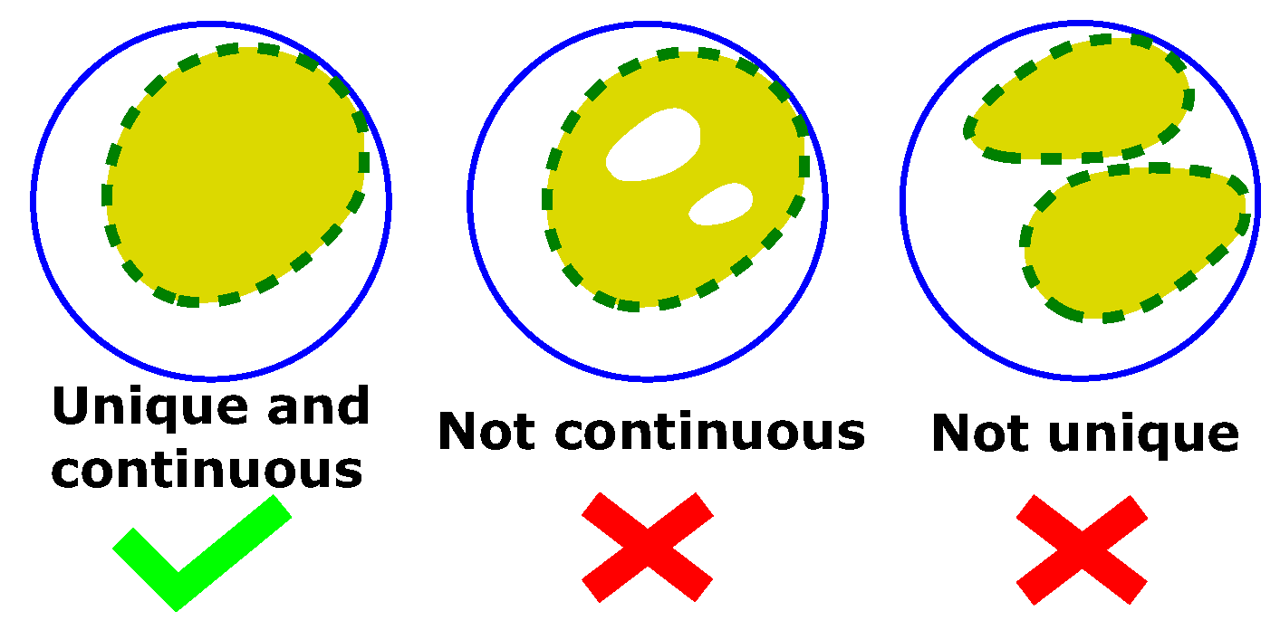
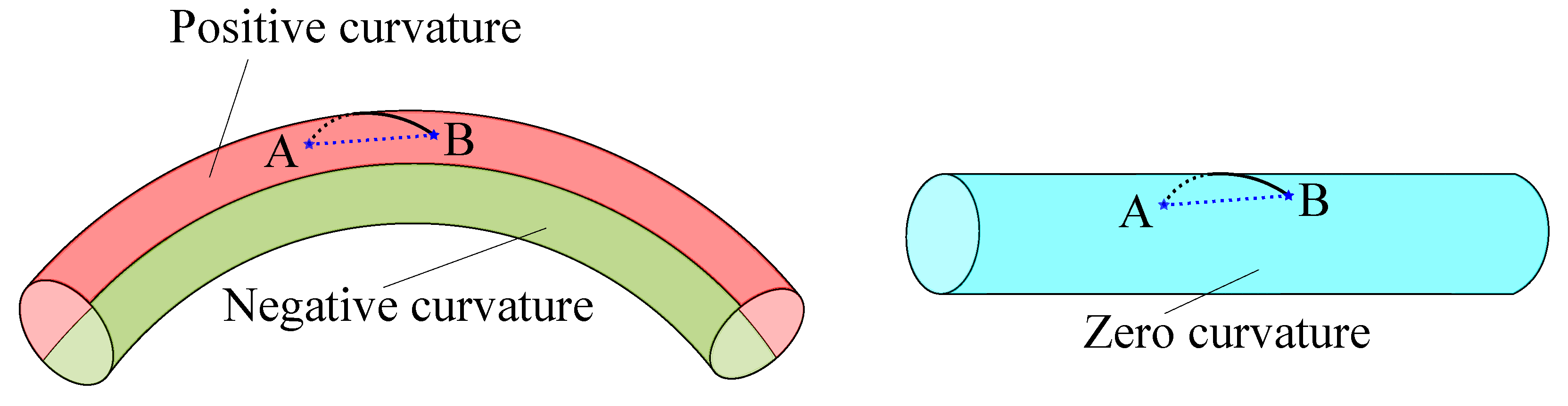
4.1. Geometric Properties of the ESP in Tubular Space

Definition 3.

For every point $\mathit{X}\in S_i\subset \mathsf{\Omega },i\ne N+1$, the cross-section $S_i$ divides Ω into two sub-spaces, and a direction from $\mathit{X}$ is said to be positive (+) if it is towards the sub-space containing the destination.

According to Definition 3, any point in $\mathsf{\Omega }$ (not belonging to $S_{N+1})$ will have an infinite number of positive directions (see Figure 3). Obviously, during the movement, the correct direction of the particle is always a positive direction.

Definition 4.

Two points $\mathit{X},\phantom{.}\mathit{Y}\in \mathsf{\Omega }$ are said to see each other if the line segment joining them $\overline{\mathit{XY}}$ is totally contained by Ω.

Definition 5.

A cross-section $S\subset \mathsf{\Omega }$ is visible from a point $\mathit{X}\in \mathsf{\Omega }$ if there exists a point $\mathit{Y}\in S$ that can be seen by $\mathit{X}$.

Lemma 2.

If a point $\mathit{X}$ inside the tube can see a cross-section S of the tube, the area part in S that can be seen by $\mathit{X}$ must be a convex set (as illustrated in Figure 4).

The proof of this lemma is detailed in Appendix A.1.

Definition 6.

From a point $\mathit{X}\in \mathsf{\Omega }$, the “length of sight” corresponding to a positive direction is the distance between $\mathit{X}$ and the farthest point in $\partial \mathsf{\Omega }$ that can be seen by $\mathit{X}$ along the positive direction. The line segment corresponding to this length is called theline of sight.

We then have the geometric structure of the shortest path between two points (which are not in each other’s line of sight) in a tubular space.

Theorem 1.

By $\mathit{f}$, we denote the shortest path between two arbitrary points $\mathit{X}$ and $\mathit{Y}$ inside the tubular space Ω. If $\mathit{X}$ cannot see $\mathit{Y}$, then there exist curved parts of $\mathit{f}$ lying on the inner lateral wall of the tube $\partial \mathsf{\Omega }$. Outside these parts, $\mathit{f}$ consists of a union of straight line segments which are tangent to the boundary surface $\partial \mathsf{\Omega }$.

Theorem 2.

The curved parts of $\mathit{f}$ are geodesic paths on $\partial \mathsf{\Omega }$. Moreover, they are on the surface of the negative curvature.

Proof. 

The proof of Theorem 1 was presented in [29]. To prove Theorem 2, we employed Lemma 1. As the curved parts of $\mathit{f}$ are also the shortest paths connecting their ends, they must be geodesic paths on the boundary surface $\partial \mathsf{\Omega }$ [37]. Moreover, if a curved path of $\mathit{f}$ exists that is outside the surface of the negative curvature, we always find on this path two neighboring points that can see each other (see Figure 5). As the straight line segment joining these points is shorter than the geodesic path between them, then $\mathit{f}$ is not the shortest one connecting $\mathit{X}$ and $\mathit{Y}$. This contradicts the definition of $\mathit{f}$ (Q.E.D.).    □

These two theorems lead us to two important corollaries.

Corollary 1.

Let $\mathit{X}$ be a point on the ESP $\mathit{p}\left(s\right)$ that can see a point $\mathit{Y}$ so that the ray $\mathit{XY}$ is not the direction $\dot{\mathit{p}}\left(s_X\right)$ of the ESP at $\mathit{X}$. Let $\left(\alpha \right)$ be an arbitrary plane containing $\mathit{XY}$. If the angle between $\dot{\mathit{p}}\left(s_X\right)$ and $\left(\alpha \right)$ is not zero, then the direction $\dot{\mathit{p}}\left(s\right)$ at any point on the ESP segment between the cross-sections containing $\mathit{X}$ and $\mathit{Y}$ will always point away from $\left(\alpha \right)$.

Proof. 

From $\mathit{X}$, the particle moves away from $\left(\alpha \right)$ (the angle between $\dot{\mathit{p}}\left(s_X\right)$ and $\left(\alpha \right)$ is not zero). Using Theorem 1, we obtain that the particle only changes its direction at points on the geodesic paths. As these curves must be on the surface of negative curvature (Theorem 2), where vector $\ddot{\mathit{p}}\left(s\right)$ points out of the tube, thus the $\dot{\mathit{p}}\left(s\right)$ will always point away from the plane $\left(\alpha \right)$ (see Figure 6).   □

Corollary 2.

If $\mathit{X}$ on the ESP can see a cross-section S of the tubular space Ω via a positive direction, the correct direction at $\mathit{X}$$\left(\dot{\mathit{p}}\left(s_X\right)\right)$ must be towards a point $\mathit{Y}$ in the visible area of S by $\mathit{X}$.

Proof. 

The above corollary can be proven by contradiction. By ${\sigma }_X\left(S\right)$, we denote the visible area of the cross-section S by $\mathit{X}$. Let $\mathit{Y}$ be the intersection of the straight line containing $\dot{\mathit{p}}\left(s_X\right)$ and the plane containing S (denoted by $\beta \left(S\right)$). We need to prove that $\mathit{Y}\in {\sigma }_X\left(S\right)$. We consider the following hypothesis of contradiction:

$$if\mathit{Y}\notin {\sigma }_X\left(S\right)\Rightarrow \overline{\mathit{XY}}\not\subset \mathsf{\Omega }$$

(4)

In other words, the ray $\mathit{XY}$ passes through the boundary $\partial \mathsf{\Omega }$. Let $\mathit{M}$ be the passing point that is closest to $\mathit{X}$. In $\beta \left(S\right)$ and through $\mathit{Y}$, we draw an arbitrary straight line that intersects with the visible area ${\sigma }_X\left(S\right)$. Let $\mathit{W}$ be the intersection point that is closest to $\mathit{Y}$. Then, $\mathit{W}$ must be on the boundary of ${\sigma }_X\left(S\right)$ (denoted by $\partial {\sigma }_X\left(S\right)$). In addition, there is a total of two relative positions of $\mathit{W}$: $\mathit{W}\in \partial \mathsf{\Omega }$ and $\mathit{W}\notin \partial \mathsf{\Omega }$ (see Figure 7). In the following, we define a plane $\left(\alpha \right)$ and a closed surface $\left(C\right)$ for these two mentioned cases:

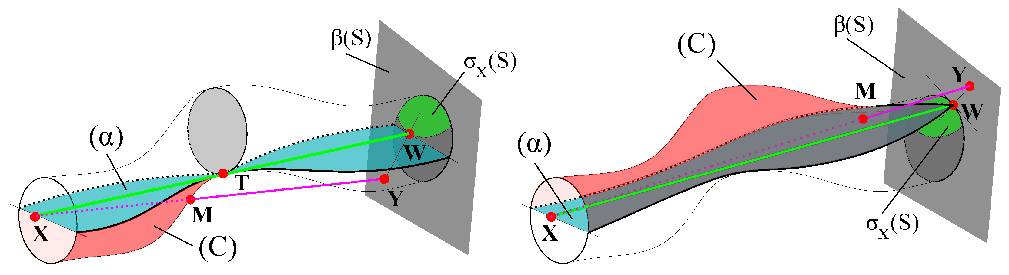
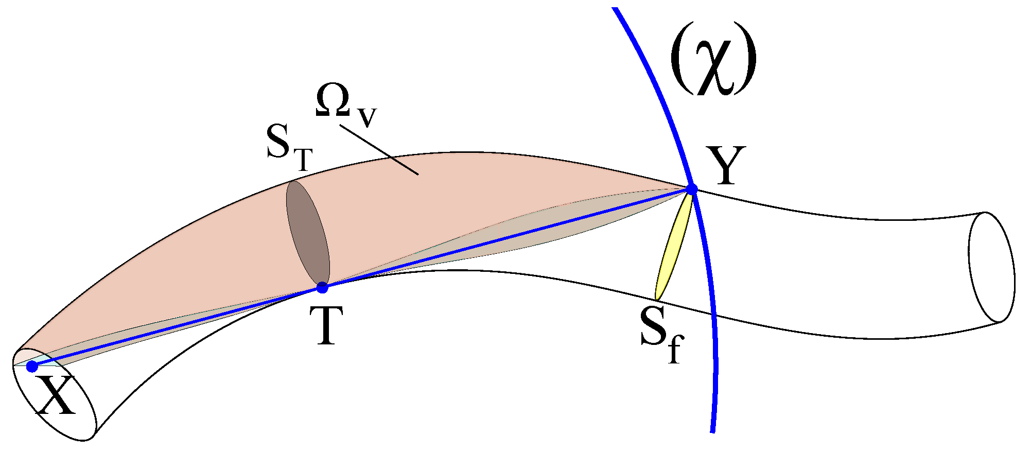
• $(\mathit{W}\notin \partial \mathsf{\Omega }$). $\left(\alpha \right)$ is the plane that contains $\mathit{XW}$ and the tangent at $\mathit{W}$ of ${\sigma }_X\left(S\right)$. If $\overline{\mathit{XW}}$ is not tangent to $\partial \mathsf{\Omega }$, we can always find in $\beta \left(S\right)$ a circle with center $\mathit{W}$ and radius $ϵ$ small enough so that the entire circle can be seen by $\mathit{X}$ (as there is no obstacle between $\mathit{X}$ and this circle). Then, there exist points outside ${\sigma }_X\left(S\right)$ (which is part of the circle) that can be seen by $\mathit{X}$. This contradicts the definition of ${\sigma }_X\left(S\right)$. Thus, $\overline{\mathit{XW}}$ is tangent to $\partial \mathsf{\Omega }$. Let $\mathit{T}$ be the tangent point that is closest to $\mathit{X}$ and $P_T(\partial \mathsf{\Omega })$ be the tangent plane of $\partial \mathsf{\Omega }$ at $\mathit{T}$. If $P_T(\partial \mathsf{\Omega })\not\equiv \left(\alpha \right)$, $P_T(\partial \mathsf{\Omega })$ will divide ${\sigma }_X\left(S\right)$ into two subsets. However, as the line of sight of a visible point in ${\sigma }_X\left(S\right)$ must pass through the cross-section of the tube at $\mathit{T}$, only then can one subset of ${\sigma }_X\left(S\right)$ be observed by $\mathit{X}$. This contradicts the definition of ${\sigma }_X\left(S\right)$. Thus, $P_T(\partial \mathsf{\Omega })\equiv \left(\alpha \right)$. We can then define a closed surface $\left(C\right)$ enclosed by $\left(\alpha \right)$, the cross-section at $\mathit{X}$, and part of $\partial \mathsf{\Omega }$ which contains $\mathit{M}$ (see Figure 7 Left).
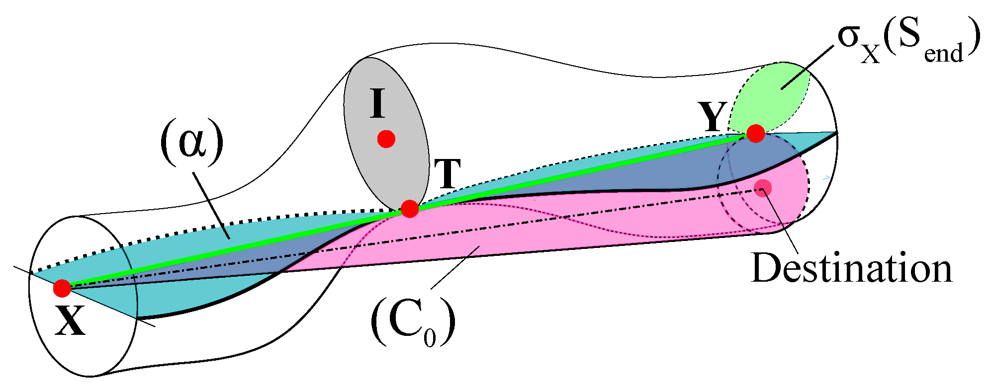
• $(\mathit{W}\in \partial \mathsf{\Omega }$). $\left(\alpha \right)$ is the plane that contains $\mathit{XW}$ and the tangent at $\mathit{W}$ of S. Then, $\left(C\right)$ is the closed surface containing $\mathit{M}$ and enclosed by $\partial \mathsf{\Omega }$, $\left(\alpha \right)$, and the cross-section of the tube at $\mathit{X}$ (see Figure 7 Right).

By using the definition of $\left(C\right)$, we can deduce from $\mathit{X}$ that the VP will go into the inner space of $\left(C\right)$. Since the destination $\mathfrak{Q}$ is outside $\left(C\right)$, the particle must pass the boundary of $\left(C\right)$ somewhere on $\left(\alpha \right)$. However, by applying Corollary 1, the direction vector $\dot{\mathit{p}}\left(s\right)$ will always point away from $\left(\alpha \right)$, thus the particle cannot return to $\left(\alpha \right)$ for a passing point. Therefore, the hypothesis (4) cannot be true, then $\mathit{Y}\in {\sigma }_X\left(S\right)$ (Q.E.D.).   □

Employing the above lemma, theorems and corollaries lead us to an important result regarding the partitions of the ESP inside a tubular space, as shown in Remark 1.

Remark 1.

For any type of tubular space, the shortest path $\mathit{p}\left(s\right)$ can be segmented into three partitions:

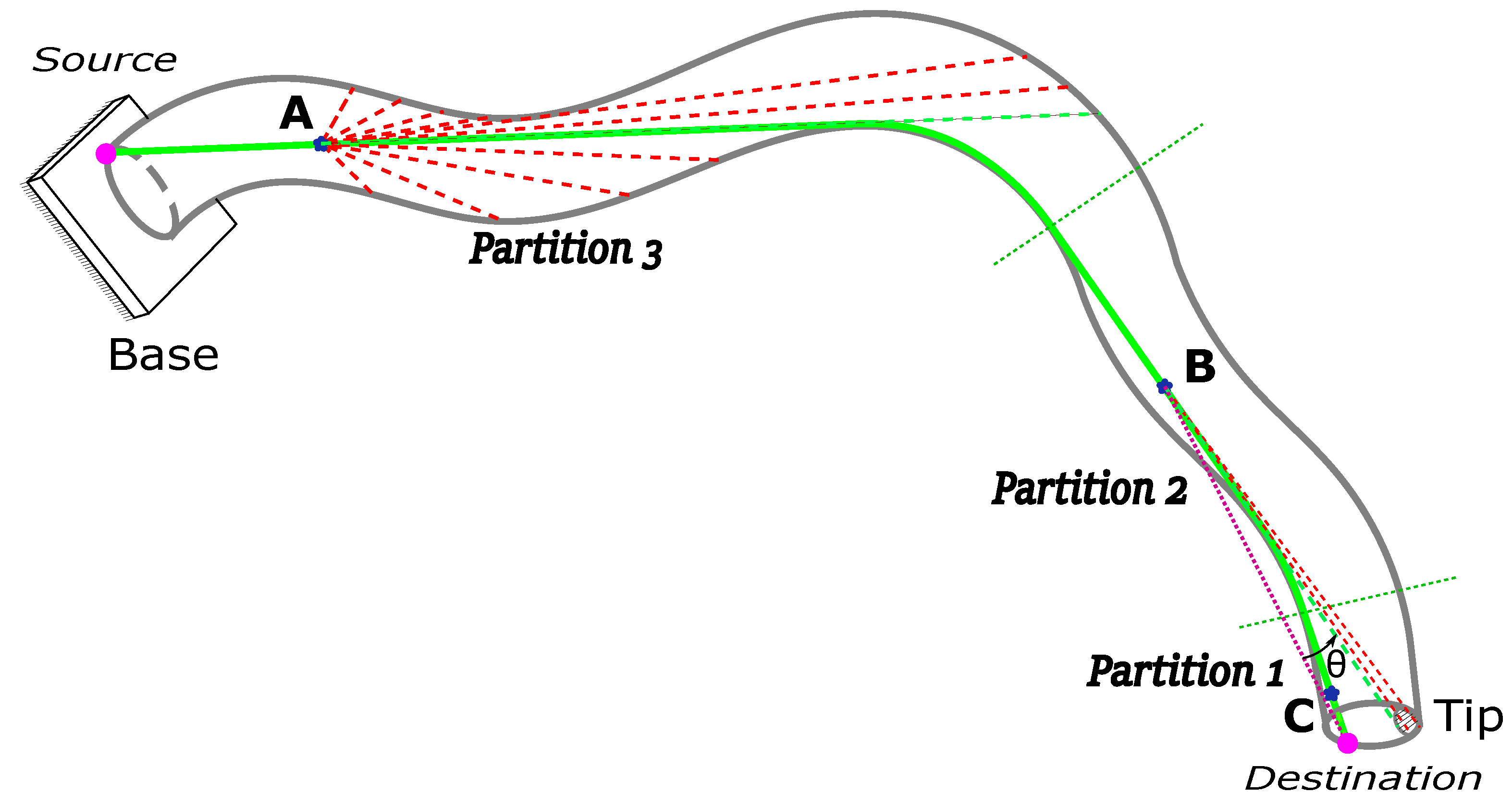
• Partition 1 (P1): Includes points that can see the destination $\mathfrak{Q}$. The direction $\dot{\mathit{p}}\left(s\right)$ at any point in this partition is always towards $\mathfrak{Q}$.
• Partition 2 (P2): Includes points that can see the ending cross-section $S_{end}$, but cannot see $\mathfrak{Q}$. The direction $\dot{\mathit{p}}\left(s\right)$ at any point $\mathit{X}$ in this partition is always towards a visible point $\mathit{Y}$ in the ending cross-section such that the angle between $\mathit{XY}$ and $\mathit{X}\mathfrak{Q}$ is the smallest one.
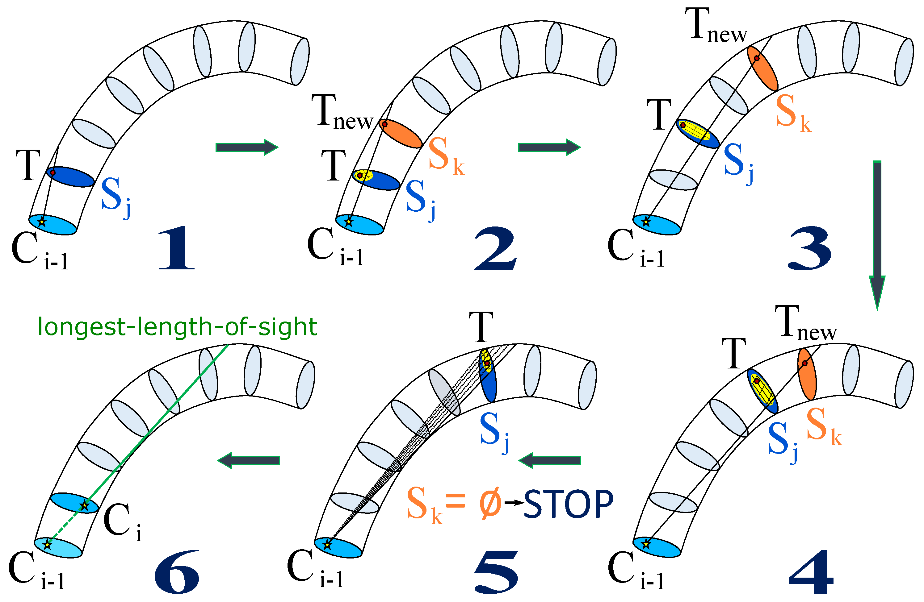
• Partition 3 (P3): Includes points that cannot see the ending cross-section $S_{end}$. The direction of $\dot{\mathit{p}}\left(s\right)$ at any point in this partition is the positive direction corresponding to the longest length of sight.

The three partitions of the searching shortest path inside the tube are described in Figure 8. The proof of this remark is given in Appendix A.2. It is important to note that a tube does not necessarily contain all three partitions. For instance, a straight tube only contains partition 1 regardless of the positions of the source and the destination.

4.2. The Proposed Algorithm

The principle of this method is based on Remark 1. Ensuring that two points can see each other in the discrete approach is equivalent to proving that the line segment joining those points must cross all the meshed circular disks between them. In the Algorithm 2, we use ${\mathit{C}}_i$ to denote the intersection point between the searching shortest path and the cross-section $S_i,i\in \left\{0,\cdots ,N+1\right\}$. The objective of Algorithm 2 is then equivalent to finding the series of ${\mathit{C}}_i$. It is important to note that ${\mathit{C}}_i$ is not necessarily a node of $G(V,A)$. Indeed, the algorithm determines the correct direction of ${\mathit{C}}_{i-1}$, thereby determining the position of ${\mathit{C}}_i$ as the intersection point between this direction and the next cross-section $S_i$. The correct direction of ${\mathit{C}}_{i-1}$ was found using Remark 1 by checking which partition ${\mathit{C}}_{i-1}$ belongs to (with precedence from P1 to P3). The value 1 of $flag$ marks that ${\mathit{C}}_{i-1}$ can see the ending cross-section $S_{N+1}$. The Oriented Drilling Process is an algorithm employed for Partition 3, which returns to the next value of the ${\mathit{C}}_i$ series by the intersection point between the longest-length-of-sight direction and the next cross-section.

Algorithm 2: Proposed method.

4.3. Oriented Drilling Process

To effectively determine the longest length of sight from an arbitrary point $\mathit{X}$ inside the tube, we employ Lemma 2. The operation scheme of finding the longest-length-of-sight direction illustrated in Figure 9 comprises a series of expanding and deepening processes. Without loss of generality, we assume that ${\mathit{C}}_{i-1}$ can see a point $\mathit{T}$ in a forward section $S_j$. By employing Lemma 2, we discretely expand the examined direction from the direction passing through $\mathit{T}$ to others passing through its nearby nodes on the same mesh $S_j$ until discovering a point ${\mathit{T}}_{new}$ in a farther disk $S_k$$(k>j)$. As a deepening process, we then update $\mathit{T}$ by ${\mathit{T}}_{new}$ and also the examined cross-section $S_j$ by $S_k$. The operation is then repeated until the expanding process is over. The condition to stop the expanding process is when the boundary of the visited area in $S_j$ just comprises the invisible nodes and the boundary points of $S_j$. Finally, we compare the length of sight corresponding to all visible points in the farthest visible cross-section and find the longest one. The next correct point ${\mathit{C}}_i$ is the intersection point between this line of sight and the next cross-section $S_i$.

One advantage of this method is the fact it represents a significant improvement in computation time as we do not need to visit all the nodes of the graph. For the expanding process, on the examined disk $S_j$, we just need to expand the investigated nodes until the current exact point ${\mathit{C}}_{i-1}$ can see farther; then we jump further into the more in-depth cross-section. Otherwise, if there is no new disk observed by ${\mathit{C}}_{i-1}$, we stop the process and indicate the next correct point of the ESP ${\mathit{C}}_i$. Moreover, as this is an inheritable algorithm, in the next searching process, we can directly use the previous correct direction as the initial examined orientation. Thus, we skip the disks that were examined in the previous loop. For several circumstances such as points on the straight-line segments of the shortest path (the ESP consists of straight-line and geodesic curve segments, see Theorems 1 and 2), the next searching process can stop right after choosing this initial examined orientation. That is also the reason why we call this method Oriented Drilling. Imagine that every time we find the correct direction for point ${\mathit{C}}_{i-1}$ such as when we drill a hole in that direction. For the next searching process, as there was already a hole, the searching is simplified. The whole process becomes an adjustment the direction of the drill so that it can drill deeper. Consequently, the drilling direction will be oriented closer and closer to the deepest drill hole (the longest length of sight).

5. Computational Results

In this section, we will compare the efficiency of the proposed algorithm with Dijkstra’s one. There are several criteria for this comparison result: the length of the obtained ESP, the computation speed, the smoothness, and the position error of the solution. The experiments were ran on a machine with an Intel Core i5-8400 CPU @ 2.80 GHz processor. It has a six-core CPU and the available RAM was 16 GB. All algorithms were implemented in Matlab. The code is available online at https://github.com/nguyengiathuongphai/ESP_Tubular.git (accessed date: 18 Feburary 2022).

5.1. Computation Time

We firstly implemented them considering a tube with the centerline in 3D space consisting of a 4 cm straight length and two curved segments belonging to two perpendicular planes. The radii of both curves are 12 cm and their lengths are 16 cm and 20 cm, respectively, as detailed in Figure 10. The inner diameter of the tube is 3 cm. We chose the discretization step h = 2 mm ($N=199$). Each meshed disk is made by dividing the cross-section into 25 concentric circles ($N_{\rho }=$ 25) whose circumference is divided into four equal arcs ($N_{\theta }=4$).

As shown in Figure 10, the proposed method enables obtaining a shorter and smoother solution than Dijkstra’s method with the same mesh (a detailed analysis will be provided in the next sub-section). Another advantage of the proposed algorithm compared to Dijkstra’s method is the computation speed as a large number of unimportant vertices and arcs can be ignored in the process (see Figure 10). As the time complexity of the proposed method has a huge variation depending on the specific shape of the tubular space, the computation time (instead of the theoretical time complexity) will be considered for the comparison result.

Table 1. Comparison result in computation time of the two methods with different meshes.

$M=100$	$N_{\rho }=25$, $N_{\theta }=4$
	T.P = 0.76, T.D = 4.10
$M=200$	$N_{\rho }=50$, $N_{\theta }=4$	$N_{\rho }=25$, $N_{\theta }=8$
	T.P = 0.96, T.D = 16.66	T.P = 1.05, T.D = 15.77
$M=400$	$N_{\rho }=100$, $N_{\theta }=4$	$N_{\rho }=25$, $N_{\theta }=16$
	T.P = 1.63, T.D = 64.67	T.P = 1.51, T.D = 60.19
$M=800$	$N_{\rho }=200$, $N_{\theta }=4$	$N_{\rho }=25$, $N_{\theta }=32$
	T.P = 3.03, T.D = 259.23	T.P = 2.01, T.D = 219.82

shows how the computation times of the two methods depend on the number of nodes in the meshed circular disks. As we can see, the computation time of Dijkstra’s method will increase by a factor of 4 if M is doubled (M is the number of nodes in a meshed disk). This is consistent with the time complexity $O\left(\right|A\left|\right)$ of Dijkstra’s algorithm ($\left|A\right|=2M+(N-1)M^2$). For the proposed method, this increasing rate is less than two.

5.2. Accuracy and Smoothness

In the following, we extend the comparison results between the two algorithms for different types of tubular spaces as shown in

Table 2. Compare the proposed method and Dijkstra’s method with many tubular surfaces.

1. Plane Parabolic Centerline	2. Plane Elliptical Centerline	3. Plane Hyperbolic Centerline
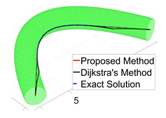L.P = 27.22, L.D = 27.29, L.E = 27.21 (cm)	L.P = 25.70, L.D = 25.74, L.E = 25.68 (cm)	L.P = 27.97, L.D = 28.10, L.E = 27.96 (cm)
T.P = 0.68, T.D = 2.57 (s)	T.P = 1.02, T.D = 2.65 (s)	T.P = 0.73, T.D = 2.64 (s)
4. Plane Sinusoidal Centerline	5. Plane Evolvent of a Circle	6. Wave-Shaped Torus on a Sphere
L.P = 24.41, L.D = 24.53, L.E = 24.39	L.P = 21.92, L.D = 21.94, L.E = 21.91	L.P = 22.29, L.D = 25.12, L.E = 21.96
T.P = 1.36 (s), T.D = 2.66	T.P = 1.16 (s), T.D = 2.57	T.P = 1.26 (s), T.D = 2.74
7. Tubular Helical Surface	8. Tubular Spiral Surface	9. Complex Shape Tubular Surface
L.P = 20.05, L.D = 20.31, L.E = 20.01	L.P = 18.87, L.D = 19.02, L.E = 18.71	L.P = 110.96, L.D = 111.22, L.E = 110.92
T.P = 1.00 (s), T.D = 2.74	T.P = 1.17 (s), T.D = 2.88	T.P = 5.90 (s), T.D = 11.29

. Depending on the properties of the centerline, we have two main classes of the tubular spaces: in plane centerline (parabolic, elliptical, hyperbolic, sinusoidal, and evolvent of a circle); and in space centerline (wave-shaped torus on a sphere, helical, spiral, and complex shape). Each meshed disk is chosen with $N_{\rho }=25$ and $N_{\theta }=4$. In all these cases, the proposed algorithm always gives shorter, smoother and faster results than Dijkstra’s algorithm with the same mesh. Unlike conventional graph-based methods (e.g., Dijkstra’s searching algorithm) in which the shortest path is made up of the graph nodes, the proposed method allows finding each correct point on the ESP by determining the intersection point between the exact moving direction (line of sight) and the next cross-section. This intersection point is not necessarily a node of the mesh and leads to a smoother and shorter solution than that by Dijkstra’s algorithm. The smoothness of this path is important, especially in mechanical applications when the derivatives of the path with respect to the arc length s of the tube is required such as using the coupled Cosserat rod and string model [38] to find the deformation of a flexible tendon drive robot in the case that the tendon locates freely inside the tube [18].

In addition to the length and the smoothness of the obtained ESP, its location inside the tube is also very important. For example, in the mechanical problem just mentioned above, the tendon location is directly related to the deformation direction of the tube. Thus, the position error of the obtained ESP to the exact solution needs to be investigated. We consider the ESPs given by Dijkstra’s and the proposed algorithms to be a series of points located on the cross-sections of the tube. Then, the position error of each point is the distance between itself and the exact solution within the containing cross-section. Let ${ϵ}_i^D$ and ${ϵ}_i^P$ be the position errors within cross-section $S_i$ of the solution by Dijkstra’s algorithm and by the proposed method, respectively. In this test, we expect to consider the relative errors instead of the absolute ones. As the obtained paths must be inside the tubular space, to limit the relative errors by 100%, we compare the absolute position error to the inner diameter of the tube d. The root mean square error (RMSE) and the maximum error ($E_{max}$) of Dijkstra’s solution are given in Equations (5) and (6) (the same for the proposed method just by replacing super index D by P):

$$\begin{array}{cc}\hfill RMS{E}^D& =\frac{1}{d}\sqrt{\frac{1}{N}\sum _{i=1}^N{\left({ϵ}_i^D\right)}^2}\hfill \end{array}$$

(5)

$$\begin{array}{cc}\hfill E_{max}^D& =\underset{i\in \{1,\cdots ,N\}}{min}\left(\frac{{ϵ}_i^D}{d}\right)\hfill \end{array}$$

(6)

Here, we do not consider the two ending cross-sections ($S_0$ and $S_{N+1}$) as the position error is obviously zero at the source and the destination. As shown in

Table 3. Root mean square and maximum position errors of the ESP obtained by the two algorithm. The tube number is as given in Table 2.

RMSE
Tube	1	2	3	4	5	6	7	8	9	Avg.
Dijkstra’s algorithm	0.506%	0.032%	1.922%	0.118%	0.007%	12.487%	1.655%	1.334%	1.140%	2.133%
Proposed algorithm	0.002%	0.002%	0.004%	0.009%	0.001%	1.003%	0.510%	0.368%	0.974%	0.319%
Maximum Error
Tube	1	2	3	4	5	6	7	8	9	Avg.
Dijkstra’s algorithm	4.343%	0.628%	11.812%	1.136%	0.226%	28.121%	8.556%	11.942%	12.017%	8.753%
Proposed algorithm	0.012%	0.016%	0.026%	0.105%	0.015%	4.774%	2.077%	2.039%	3.782%	1.427%

, the proposed method always provides smaller $RMSE$ and $E_{max}$ than those obtained by Dijkstra’s algorithm for all of the tubes. Concretely, the average values among these tubes of $RMSE$ and of $E_{max}$ for the proposed solution are, respectively, $0.319\%$ and $1.427\%$ and approximately six times smaller than those given by Dijkstra’s algorithm ($2.133\%$ and $8.753\%$, respectively). As the path obtained by Dijkstra’s method must pass through nodes of the weighted graph, its position errors significantly depend on the meshing. These errors can be reduced if we increase the granularity of the mesh, but it will also increase the computation time. For the proposed method, the location of the obtained path is not forced to be the nodes of the graph that leads to smaller position errors.

To extend the comparison results for different granularities of the meshed disks, Tube 6 (wave-shaped torus on a sphere) and Tube 7 (helical tubular surface) will be considered. The mesh is modified using different $N_{\rho }$ and $N_{\theta }$ as shown in

Table 4. Comparison results between the proposed algorithm and Dijkstra’s algorithm with different granularities of the meshed cross-sections of the tube.

		${\mathit{N}}_{\mathit{\rho }}=5$				${\mathit{N}}_{\mathit{\rho }}=20$
		${\mathit{N}}_{\mathit{\theta }}=\mathit{4}$	${\mathit{N}}_{\mathit{\theta }}=\mathit{16}$	${\mathit{N}}_{\mathit{\theta }}=\mathit{32}$	${\mathit{N}}_{\mathit{\theta }}=\mathit{64}$	${\mathit{N}}_{\mathit{\theta }}=\mathit{4}$	${\mathit{N}}_{\mathit{\theta }}=\mathit{16}$	${\mathit{N}}_{\mathit{\theta }}=\mathit{32}$	${\mathit{N}}_{\mathit{\theta }}=\mathit{256}$
Tube 6	L.P (cm)	22.28	22.35	22.29	22.27	22.32	22.37	22.44	22.26
	L.D (cm)	25.83	25.83	25.83	23.74	25.18	25.18	25.18	22.05
	${\mathrm{RMSE}}^{\mathrm{P}}$ (%)	1.05	1.34	0.77	0.71	1.13	1.70	1.72	0.89
	${\mathrm{RMSE}}^{\mathrm{D}}$ (%)	13.58	13.58	13.58	2.90	12.00	12.00	12.00	0.30
	T.P (s)	0.45	0.78	1.18	1.82	0.86	1.70	2.73	17.01
	T.D (s)	0.16	1.54	5.70	22.00	1.66	21.38	82.90	5582.00
Tube 7	L.P (cm)	20.06	20.04	20.04	20.08	20.05	20.05	20.04	20.08
	L.D (cm)	20.82	20.82	20.82	20.82	20.32	20.32	20.32	20.09
	${\mathrm{RMSE}}^{\mathrm{P}}$ (%)	0.62	0.14	0.30	0.73	0.55	0.17	0.20	0.59
	${\mathrm{RMSE}}^{\mathrm{D}}$ (%)	2.92	2.92	2.92	2.92	1.61	1.61	1.61	0.06
	T.P (s)	0.31	0.60	0.85	1.34	0.66	1.15	1.67	7.67
	T.D (s)	0.15	1.52	5.58	21.82	1.63	21.89	84.34	5585.00

. In these tests, the path length given by the proposed method are shorter than that proposed by Dijkstra’s algorithm for most cases. As a consequence, the proposed method also provides solutions with smaller position errors in comparison with Dijkstra’s algorithm. Even so, for the mesh with high granularity ($N_{\rho }=20,N_{\theta }=256$), Dijkstra’s algorithm can give a more accurate result than that obtained by the proposed method but it requires a much longer computation time. The accuracy of Dijkstra’s solution increases with the increase in $N_{\rho }$ and $N_{\theta }$ while this is not always true with the proposed method. The reason is that a sparse grid can effectively constrain the movement of the VP in the correct direction in some cases. The proposed solution may become more wavy with a higher granular mesh. However, the length of the obtained paths only fluctuate in a narrow range ($\pm 0.5\%$ for Tube 6) and ($\pm 0.1\%$ for Tube 7). Eventually, when the number of nodes on the mesh is higher, the increasing rate in the computation time of Dijkstra’s algorithm is superior to that of the proposed method.

6. Discussion

In this section, the extended application scope of the proposed algorithm and the ability to apply it as a reactive method for the navigation problem in unknown environments will be discussed.

6.1. Extended Applications

We can extend the application scope of the proposed method for general tunnels with convex and variable cross-sections (see Figure 11). Indeed, with a minor modification on Remark 1 for points in P3, the correct direction is towards the (only) visible point of the farthest visible cross-section instead of considering the longest length of sight, one can confirm that the correctness of Remark 1 will still be preserved (see the Appendix A.2).

6.2. A Reactive Method

In this work, we used the same directed graph for Dijkstra’s algorithm and the proposed algorithm for the aim of simplifying the validation and the comparison results. It is important to note that the proposed method does not require knowledge of the entire volume $\mathsf{\Omega }$ to obtain a weighted graph before searching. In fact, the correct direction of the particle can be determined based on the observation in front of it. While using Dijkstra’s algorithm, we cannot determine which path is the ESP until visiting all nodes and arcs of the graph; since we need to store all possible paths during the operation, the proposed method enables us to directly generate the motion decision during the movement there by the ESP is gradually traced by the moving path of the VP. Thus, it can be applied as a reactive method for robots that need to explore unknown tubular spaces such as lava tubes on an astronomical object [39] or environments in the absence of GPS signals [40]. In practice, the proposed algorithm should be run together with a given safety boundary constraint to prevent collision with inspection robots.

7. Conclusions

In this paper, we presented a novel algorithm for solving the ESP problem inside tubular spaces based on its geometric properties. Computational results were obtained for various types of tubular spaces. We demonstrated that the achieved efficiency of the proposed algorithm is better than that of Dijkstra’s algorithm. Concretely, the proposed method provided smoother and more precise results with a faster calculation speed than one obtained by Dijkstra’s algorithm with the same grid. The strength of the proposed method is also reflected in the fact that it can work without knowing the environment in advance, which allows it to process as a reactive method. Even though the algorithm was described for the tubular space, it is also strongly promising for more complex tunnel spaces to which it can directly be applied with the aforementioned minor modification. A limitation of this method is that it is only applicable to unbranched tubular spaces. In order to apply this method for a branched tubular space, additional information will be required to make decisions at the junctions of branches.

As the ESP may lie on the tubular surface, the requirement of using a collision-free method together with the proposed algorithm has been left for future research. Our plans for future work concern some applications such as the online trajectory generation of navigation robots in unknown tunnels or determine the deformation of a tendon-driven tube-like robot in medical applications, which are also included in our domain of interest.

References

- Li, F.; Klette, R. Euclidean shortest paths. In Euclidean Shortest Paths; Springer: Berlin/Heidelberg, Germany, 2011; pp. 3–29. [Google Scholar]
- Özaslan, T.; Shen, S.; Mulgaonkar, Y.; Michael, N.; Kumar, V. Inspection of penstocks and featureless tunnel-like environments using micro UAVs. In Field and Service Robotics; Springer: Berlin/Heidelberg, Germany, 2015; pp. 123–136. [Google Scholar]
- Özaslan, T.; Mohta, K.; Keller, J.; Mulgaonkar, Y.; Taylor, C.J.; Kumar, V.; Wozencraft, J.M.; Hood, T. Towards fully autonomous visual inspection of dark featureless dam penstocks using MAVs. In Proceedings of the 2016 IEEE/RSJ International Conference on Intelligent Robots and Systems (IROS), Daejeon, Korea, 9–14 October 2016; pp. 4998–5005. [Google Scholar]
- Özaslan, T.; Loianno, G.; Keller, J.; Taylor, C.J.; Kumar, V.; Wozencraft, J.M.; Hood, T. Autonomous navigation and mapping for inspection of penstocks and tunnels with MAVs. IEEE Robot. Autom. Lett. 2017, 2, 1740–1747. [Google Scholar] [CrossRef]
- Quenzel, J.; Nieuwenhuisen, M.; Droeschel, D.; Beul, M.; Houben, S.; Behnke, S. Autonomous MAV-based indoor chimney inspection with 3D laser localization and textured surface reconstruction. J. Intell. Robot. Syst. 2019, 93, 317–335. [Google Scholar] [CrossRef]
- Petrlík, M.; Báča, T.; Heřt, D.; Vrba, M.; Krajník, T.; Saska, M. A Robust UAV System for Operations in a Constrained Environment. IEEE Robot. Autom. Lett. 2020, 5, 2169–2176. [Google Scholar] [CrossRef]
- Shukla, A.; Karki, H. Application of robotics in onshore oil and gas industry—A review Part I. Robot. Auton. Syst. 2016, 75, 490–507. [Google Scholar] [CrossRef]
- Chataigner, F.; Cavestany, P.; Soler, M.; Rizzo, C.; Gonzalez, J.P.; Bosch, C.; Gibert, J.; Torrente, A.; Gomez, R.; Serrano, D. Arsi: An aerial robot for sewer inspection. In Advances in Robotics Research: From Lab to Market; Springer: Berlin/Heidelberg, Germany, 2020; pp. 249–274. [Google Scholar]
- Tan, C.H.; Ng, M.; Shaiful, D.S.B.; Win, S.K.H.; Ang, W.; Yeung, S.K.; Lim, H.; Do, M.N.; Foong, S. A smart unmanned aerial vehicle (UAV) based imaging system for inspection of deep hazardous tunnels. Water Pract. Technol. 2018, 13, 991–1000. [Google Scholar] [CrossRef]
- Tan, C.H.; bin Shaiful, D.S.; Ang, W.J.; Win, S.K.H.; Foong, S. Design optimization of sparse sensing array for extended aerial robot navigation in deep hazardous tunnels. IEEE Robot. Autom. Lett. 2019, 4, 862–869. [Google Scholar] [CrossRef]
- Mallios, A.; Ridao, P.; Ribas, D.; Carreras, M.; Camilli, R. Toward autonomous exploration in confined underwater environments. J. Field Robot. 2016, 33, 994–1012. [Google Scholar] [CrossRef] [Green Version]
- Fairfield, N.; Kantor, G.; Wettergreen, D. Real-time SLAM with octree evidence grids for exploration in underwater tunnels. J. Field Robot. 2007, 24, 03–21. [Google Scholar] [CrossRef] [Green Version]
- Gary, M.; Fairfield, N.; Stone, W.C.; Wettergreen, D.; Kantor, G.; Sharp, J.M., Jr. 3D Mapping and Characterization of Sistema Zacatón from DEPTHX (DE ep P hreatic TH ermal e X plorer). In Proceedings of the ASCE 11th Sinkhole Conference (KARST ’08), Tallahassee, Florida, 22–26 September 2008; pp. 202–212. [Google Scholar]
- Pidic, A.; Aasbøe, E.; Almankaas, J.; Wulvik, A.; Steinert, M. Low-Cost Autonomous Underwater Vehicle (AUV) for Inspection of Water-Filled Tunnels During Operation. In Proceedings of the International Design Engineering Technical Conferences and Computers and Information in Engineering Conference, Quebec City, QC, Canada, 26–29 August 2018. [Google Scholar]
- Alvarez, A.; Caiti, A.; Onken, R. Evolutionary path planning for autonomous underwater vehicles in a variable ocean. IEEE J. Ocean. Eng. 2004, 29, 418–429. [Google Scholar] [CrossRef]
- Gao, X.Z.; Hou, Z.X.; Zhu, X.F.; Zhang, J.T.; Chen, X.Q. The shortest path planning for manoeuvres of UAV. Acta Polytech. Hung. 2013, 10, 221–239. [Google Scholar]
- Dang, T.; Mascarich, F.; Khattak, S.; Nguyen, H.; Nguyen, H.; Hirsh, S.; Reinhart, R.; Papachristos, C.; Alexis, K. Autonomous search for underground mine rescue using aerial robots. In Proceedings of the 2020 IEEE Aerospace Conference, Big Sky, Montana, 7–14 March 2020; pp. 1–8. [Google Scholar]
- Swaney, P.J.; York, P.A.; Gilbert, H.B.; Burgner-Kahrs, J.; Webster, R.J. Design, fabrication, and testing of a needle-sized wrist for surgical instruments. J. Med. Devices 2017, 11, 014501. [Google Scholar] [CrossRef] [PubMed] [Green Version]
- Nguyen, D.-V.-A.; Girerd, C.; Boyer, Q.; Rougeot, P.; Lehmann, O.; Tavernier, L.; Szewczyk, J.; Rabenorosoa, K. A Hybrid Concentric Tube Robot for Cholesteatoma Laser Surgery. IEEE Robot. Autom. Lett. 2022, 7, 462–469. [Google Scholar] [CrossRef]
- Canny, J.; Reif, J. New lower bound techniques for robot motion planning problems. In Proceedings of the 28th Annual Symposium on Foundations of Computer Science (sfcs 1987), Los Angeles, CA, USA, 12–14 October1987; pp. 49–60. [Google Scholar]
- Sharir, A.; Baltsan, A. On shortest paths amidst convex polyhedra. In Proceedings of the second annual symposium on Computational Geometry, Yorktown Heights, NY, USA, 2–4 June 1986; pp. 193–206. [Google Scholar]
- Gewali, L.P.; Ntafos, S.; Tollis, I.G. Path planning in the presence of vertical obstacles. IEEE Trans. Robot. Autom. 1990, 6, 331–341. [Google Scholar] [CrossRef]
- Agarwal, P.K.; Sharathkumar, R.; Yu, H. Approximate Euclidean shortest paths amid convex obstacles. In Proceedings of the Twentieth Annual ACM-SIAM Symposium on Discrete Algorithms, SIAM, New York, NY, USA, 4–6 January 2009; pp. 283–292. [Google Scholar]
- Mitchell, J.S. Geometric Shortest Paths and Network Optimization. Handb. Comput. Geom. 2000, 334, 633–702. [Google Scholar]
- Deschamps, T.; Cohen, L.D. Fast extraction of minimal paths in 3D images and applications to virtual endoscopy. Med. Image Anal. 2001, 5, 281–299. [Google Scholar] [CrossRef] [Green Version]
- Bulow, T.; Klette, R. Digital curves in 3D space and a linear-time length estimation algorithm. IEEE Trans. Pattern Anal. Mach. Intell. 2002, 24, 962–970. [Google Scholar] [CrossRef]
- Li, F.; Klette, R. Rubberband algorithms for solving various 2D or 3D shortest path problems. In Proceedings of the 2007 International Conference on Computing: Theory and Applications (ICCTA’07), Kolkata, India, 5–7 March 2007; pp. 9–19. [Google Scholar]
- Dogan, F.; Yayli, Y. On the curvatures of tubular surface with Bishop frame. Commun. Fac. Sci. Univ. Ank. Ser. A1 Math. Stat. 2011, 60, 59–69. [Google Scholar]
- Chow, S.N.; Lu, J.; Zhou, H.M. Finding the shortest path by evolving junctions on obstacle boundaries (E-JOB): An initial value ODEś approach. Appl. Comput. Harmon. Anal. 2013, 35, 165–176. [Google Scholar] [CrossRef]
- Elmokadem, T.; Savkin, A.V. A method for autonomous collision-free navigation of a quadrotor UAV in unknown tunnel-like environments. Robotica 2021, 1–27. [Google Scholar] [CrossRef]
- Moore, E.F. The shortest path through a maze. Proc. Int. Symp. Switching Theory 1959, 1959, 285–292. [Google Scholar]
- Dijkstra, E.W. A note on two problems in connexion with graphs. Numer. Math. 1959, 1, 269–271. [Google Scholar] [CrossRef] [Green Version]
- Savkin, A.V.; Hoy, M. Reactive and the shortest path navigation of a wheeled mobile robot in cluttered environments. Robotica 2013, 31, 323–330. [Google Scholar] [CrossRef]
- Hachour, O. The use of the 3D Smoothed parametric curve Path planning for Autonomous mobile robots. Int. J. Syst. Appl. Eng. Dev. 2009, 3, 105–116. [Google Scholar]
- Blaga, P.A. On tubular surfaces in computer graphics. Stud. Univ. Babes-Bolyai Inform. 2005, 50, 81–90. [Google Scholar]
- Hart, P.E.; Nilsson, N.J.; Raphael, B. A formal basis for the heuristic determination of minimum cost paths. IEEE Trans. Syst. Sci. Cybern. 1968, 4, 100–107. [Google Scholar] [CrossRef]
- Bose, P.; Maheshwari, A.; Shu, C.; Wuhrer, S. A survey of geodesic paths on 3D surfaces. Comput. Geom. 2011, 44, 486–498. [Google Scholar] [CrossRef] [Green Version]
- Rucker, D.C.; Webster, R.J., III. Statics and dynamics of continuum robots with general tendon routing and external loading. IEEE Trans. Robot. 2011, 27, 1033–1044. [Google Scholar] [CrossRef]
- Thangavelautham, J.; Robinson, M.S.; Taits, A.; McKinney, T.; Amidan, S.; Polak, A. Flying, hopping Pit-Bots for cave and lava tube exploration on the Moon and Mars. arXiv 2017, arXiv:1701.07799. [Google Scholar]
- am Ende, B. 3D mapping of underwater caves. IEEE Comput. Graph. Appl. 2001, 21, 14–20. [Google Scholar] [CrossRef]
- Boyd, S.; Boyd, S.P.; Vandenberghe, L. Convex Optimization; Cambridge University Press: Cambridge, UK, 2004. [Google Scholar]