Abstract
The accurate estimation of how future demand will react to prices is central to the optimization of pricing decisions. The systems responsible for demand prediction and pricing optimization are called revenue management (RM) systems, and, in the airline industry, they play an important role in the company’s profitability. As airlines’ current pricing decisions impact future knowledge of the demand behavior, the RM systems may have to compromise immediate revenue by efficiently performing price experiments with the expectation that the information gained about the demand behavior will lead to better future pricing decisions. This earning while learning (EWL) problem has captured the attention of both the industry and academia in recent years, resulting in many proposed solutions based on heuristic optimization. We take a different approach that does not depend on human-designed heuristics. We present the EWL problem to a reinforcement learning agent, and the agent’s goal is to maximize long-term revenue without explicitly considering the optimal way to perform price experimentation. The agent discovers through experience that “myopic” revenue-maximizing policies may lead to a decrease in the demand model quality (which it relies on to take decisions). We show that the agent finds novel pricing policies that balance revenue maximization and demand model quality in a surprisingly effective way, generating more revenue over the long run than current practices.
1. Introduction
Revenue management (RM) practices are very important for airlines and many other industries, such the as car rental, hotel, retail industries, etc. Perhaps one of the most remarkable aspects of RM is how much airline companies must price their products to maximize their revenue. By setting the prices too high for its products, an airline may drive away potential customers, conversely by choosing to price too low, it may lose potential profits. These pricing decisions are often critical to the airline’s success.
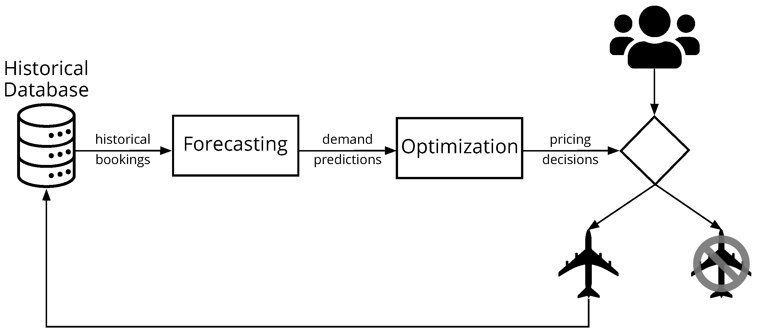
The optimization of pricing decisions is usually delegated to a specialized revenue management system (RMS). The RMS first calibrates, from historical booking data, the parameters of a demand model that forecasts how future demand will answer to prices, then the forecast is used to optimize the pricing policy that indicates how to vary prices according to the airline’s current inventory capacity. Only the booking decisions made by customers are stored in a fixed-size historical database for future use (no-booking decisions cannot be captured by airlines), and the oldest records are deleted (first-in, first-out). Figure 1 illustrates the process.
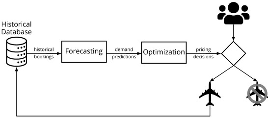
Figure 1.
Inside revenue management systems.
The quality of the prediction of future demand obtained by the calibrated demand model is fundamental to price optimization. For example, in the airline industry, it has been calculated that a bias of in the estimation of the demand price sensitivity (i.e., how the expected demand increases or decreases with respect the offered price) can reduce revenue by up to [1]. Optimizing pricing decisions under the assumption that the demand behavior is unknown, which must be discovered from historical data, has come to be known as the “earning while learning” (EWL) problem. At every moment, the airline faces a choice of selecting the “perceived” optimal price that maximizes revenue according to its current beliefs or selecting another price that increases the amount of information the airline has about the demand behavior.
The EWL problem has attracted strong interest from academia and the airline industry in recent years, most notably after the COVID-19 pandemic, when demand behavior changed significantly from historical behavior as a consequence of an important shift in competitor presence and customer interests [2,3,4,5]. Even though we only consider stationary demand in this work (i.e., no shocks), we believe that many changes in RMSs will be needed to efficiently rediscover new demand behavior during the following years of recovery, effective price experimentation being perhaps one of the most important pieces of the puzzle. Even though the research performed for this study can be extended to the case of market shocks, for simplicity we analyze its performance in well-understood stationary environments, i.e., where the amount of data collected from interactions with the demand is limited.
Most of the work conducted with the aim of solving the EWL problem relies on expert-designed heuristics. Some of these heuristics are very effective; however, they often come with constraints that make them difficult to apply to real-world airline RM. RMSs use complex optimization methods to adjust prices according to a flight’s remaining inventory capacity, requiring such heuristics to be adaptable to the optimization method that is being used. Moreover, airlines manage several flights simultaneously (e.g., daily flights between destinations), and the booking data of each flight are appended to the historical database and used for demand model estimation, suggesting that the heuristic methods need to adapt price experimentation across many concurrent flights.
Similar questions to the EWL problem arise in the literature of statistics as optimal experimental design, or in machine learning as active learning [6], or in the field of reinforcement learning (RL) as the exploration–exploitation trade-off [7]. In fact, many of the heuristic methods tackling the EWL problem take inspiration from other disciplines, such as Thompson sampling [8], upper confidence bound [9], and many others. Nonetheless, the methods that arise from these disciplines are based on heuristics. Instead, in this work, we take a different approach.
Given the success of artificial intelligence (AI) in recent years [10,11,12] and inspired by the “reward is enough” hypothesis [13], we demonstrate that an RL agent can discover solutions to the EWL problem without any guidance from human-designed heuristics. We show that the RL agent develops pricing policies that generate more long-term revenue than state-of-the-art heuristic methods, while effectively controlling the uncertainty of the unknown model parameters of the demand function.
This work makes major contributions to how RL is applied to RM and to the EWL problem. RL is often seen as an online model-free alternative to RMSs that traditionally require a demand model [14,15,16]. The issue with such an approach is that data from real customers are not abundant enough to perform online training, and model-free RL methods are shown to be far less data efficient than model-based RMSs. Instead, we propose to use a sample model of the demand for offline training [10,17], thus focusing on the improvement of the pricing optimization only. Furthermore, we also call attention to the continuing nature of the EWL problem; balancing between earning and learning is a task that never finishes. In contrast to the optimization of the episodic revenue performed by RMSs (which maximizes the revenue of each flight, ignoring long term consequences of learning), we present an alternative modeling of the problem that maximizes the revenue of all concurrent flights in a combined way, allowing us to express the system’s revenue-maximization objective over an infinite horizon. Then, we demonstrate how to adapt RL to optimize the pricing policy for this new objective through the average reward.
In Section 2, we overview the algorithms proposed in literature for solving the EWL problem. Next, in Section 3, we briefly introduce the monopolistic single-leg problem and how price optimization is typically performed by RMSs in this problem. In the same Section, we also review some basic concepts behind RL that we believe to be required for understanding our method. Then, in Section 4, we present how to formulate the EWL problem so it can be addressed by an RL agent. Following this, in Section 5, we present comparative simulation studies between the heuristic methods and the solution found by RL. To demonstrate the ability of the RL agent to solve more complex and realistic settings, we compare RL to traditional RMS in scenarios where the heuristic methods are not defined. We close this work with a discussion about our method in Section 6, and we present our vision for future research in Section 7.
2. Heuristic Methods for Earning While Learning
The EWL problem has its roots into the research fields of price optimization and optimal control (earning), and statistical learning and economics (learning about the demand behavior). Even though these research fields are each more than a century old, they were studied independently for a long time. The first attempts to combine these two fields [18,19] did not receive much attention, perhaps due to the technical difficulties of the time, such as implementing pricing variation (e.g., updating catalogs), obtaining reliable estimates of the demand behavior, and tracking competition pricing. It was not until the digital and information era, when changing prices and accurately keeping track of how demand responds to them became much more effective, that academia and industry started to pay attention to the EWL problem.
The literature of EWL is often organized based on how learning about the demand behavior happens. Many papers that investigate the EWL problem assume that the unknown demand behavior parameters are learned by the decision maker through the Bayesian framework [20,21,22], while others concentrate on the parametric framework [23,24], and yet some others are oriented towards non-parametric models [25,26]. Even though we have a special interest in the parametric model framework, many important discoveries generalize across frameworks, and thus we present them below.
One of the most influential early works addressing the EWL problem proposes to learn the demand model parameters in a Bayesian fashion [27]. In theory, the optimal Bayesian policy could be computed via dynamic programming, but, in many situations of interest, no closed-form analytical expression exists. Thus, the proposed workaround, today known as certainty equivalent pricing (CEP), consists of selecting at each time step the price that would be optimal if the current demand model parameter estimates were correct. CEP is shown to be optimal under certain conditions, such as when only the intersect of a linear demand function is being estimated, but it is sub-optimal when estimating both the slope and the intersect of a linear demand model [28]. However, further analytical studies [29,30] pointed to a more fundamental problem: the sequence of prices may converge to a sub-optimal price even with infinite data. This phenomenon has been named incomplete learning, and it has been demonstrated theoretically that, to avoid incomplete learning while maximizing revenue, the system must follow a policy that accumulates information about the demand behavior at an adequate rate without deviating too much from the greedy policy [24]. Several heuristic methods combining this principle with a classical parametric demand model [4,8,20,31,32] have been studied, in which controlled variance pricing (CVP) [2] has arguably been the most influential method. The CVP algorithm imposes a constraint on the greedy pricing policy that requires the selected prices not be too close to the average of previously selected prices. This constraint seeks to guarantee sufficient price dispersion by imposing a “taboo interval” over prices which the system is not allowed to select.
Recently, a novel heuristic method [3] was found to outperform CVP in simulated studies and real-world benchmarks. This heuristic combines the revenue maximization and the accumulation of information into a single objective function in the form of
where is the trade-off parameter, represents the expected revenue for fare f, and represents uncertainty of the demand behavior after selecting fare f. At each time step, the system selects the fare that maximizes the objective function . The main idea of this heuristic is to include the uncertainty of the demand model parameters in the optimization objective as a penalty term. If the uncertainty over the parameters becomes too large, the system shifts from a revenue-maximizing to an information-maximizing fare. The trade-off parameter, , can be used to tune the importance that the system should pay to the uncertainty of the demand model parameters. In a recent study, this method was successfully adapted to airline RM under the assumption of unconstrained capacity (i.e., infinite inventory capacity) [33], making it only useful for flights with small load factors (flights that have much more capacity than demand).
Another stream of research brings to the light the similarities between the EWL problem and questions that arise in the field of machine learning, such as active learning [34] and the exploration–exploitation trade-off [30,35,36]. The literature around these topics is large, where some of the most popular techniques are Thompson sampling [37], upper confidence bound [38], the /R-max algorithms [39,40], and intrinsic curiosity [41]. However, in the EWL problem, a model of the demand behavior is present, and the model describes how each possible price relates to the others. This is very different from solving the exploration–exploitation trade-off in the general case, which often assumes that each possible choice delivers a response independent of the others. The ability to exploit the existence of a demand model is key for solving the EWL problem.
We organize the key studies in Table 1 with respect to the important requirements we believed to be needed to a successful integration with airline RM. For the first requirement, we seek methods that are directly compatible with parametric demand models. Furthermore, these methods need to either consider pricing under limited inventory capacity, or they need to be adaptable to current practices for pricing optimization. For our last requirement, the methods need to consider that the historical booking data are generated by many flights simultaneously (multi-flight), or they need to be easily integrated to this scenario. These three requirements sum up the core conditions to apply the earning-while-learning methods to airline RM.

Table 1.
Earning-while-learning literature review.
In summary, due to the absence of a general well-defined tractable optimization objective, the EWL literature has focused on finding human-designed heuristic methods for balancing between revenue maximization on one hand and model learning on the other. In the next sections, we present a novel method going beyond these human-designed heuristics. We demonstrate that, using RL, we can discover more effective pricing policies directly from the maximization of the standard reward signal (i.e., pure revenue maximization without any engineering of the reward signal) in the challenging single-leg problem.
3. Background
This section is devoted to the description of the single-leg problem and how it is typically solved. We also briefly review important concepts concerning RL that will be used throughout this work.
3.1. The Single-Leg Problem
We consider the monopolistic, capacity-constrained single-leg problem. In this problem, there is only one airline operating a single leg from point A to point B. Every day a new flight is open for sale and another flight departs, closing for new bookings. Each flight is open for sale days prior to departure (also called the booking horizon), and the airline must manage active flights simultaneously. The customers are only willing to book the flight departing on a specific day, and they either choose to book or not to book at all. The RMS’s goal, then, is to select the prices for every active flight so as to maximize the airline’s long-term revenue. For simplicity, we assume that overbooking and cancellations are not possible and that the flight has a single cabin class (e.g., first class, business, or economy), with C being the flight’s capacity for this unique cabin. We consider that the RMS must select the prices from a discrete fare structure , where is a price point. Furthermore, for the sake of generality, from now on we call a “day” a “time step” (because in principle it could be any unit of time).
We assume that demand behaves according to a parametric demand function that returns the expected number of customers willing to pay for fare f, and represents a generic set of parameters of the demand function. A demand model extensively used in the literature is the exponential model [14,42], with , given by
where customers arrive according to a Poisson distribution with mean , called the arrival rate parameter, and is the price sensitivity parameter. The constant is the lowest fare in the fare structure such that the customer’s purchase probability is one . Perhaps the most straightforward way to simulate this demand model consists of generating customer arrivals for each time step according to the Poisson distribution, and, for each arriving customer, we sample a random value between zero and one, and, if the sampled value is smaller than the purchase probability at the selected fare f, the customer accepts the offer, proceeding with the purchase, otherwise the customer rejects the offer, and no booking is made.
As the true demand behavior is unknown by the RMS, it must estimate the demand model parameters from historical booking data, which can be performed with an ordinary least squares or a maximum likelihood estimation [33,43].
Next, the RMS uses the calibrated demand model to optimize the pricing policy for each active flight independently of the others. This pricing policy adjusts the price according to flight’s current inventory state (e.g., the remaining capacity and the time steps to departure), that is, when the flight has excess capacity, the policy may decrease prices aiming to capture more customers, on the contrary, when the flight has a deficit of capacity, the policy may increase prices aiming to capture only customers that are willing to book at higher prices.
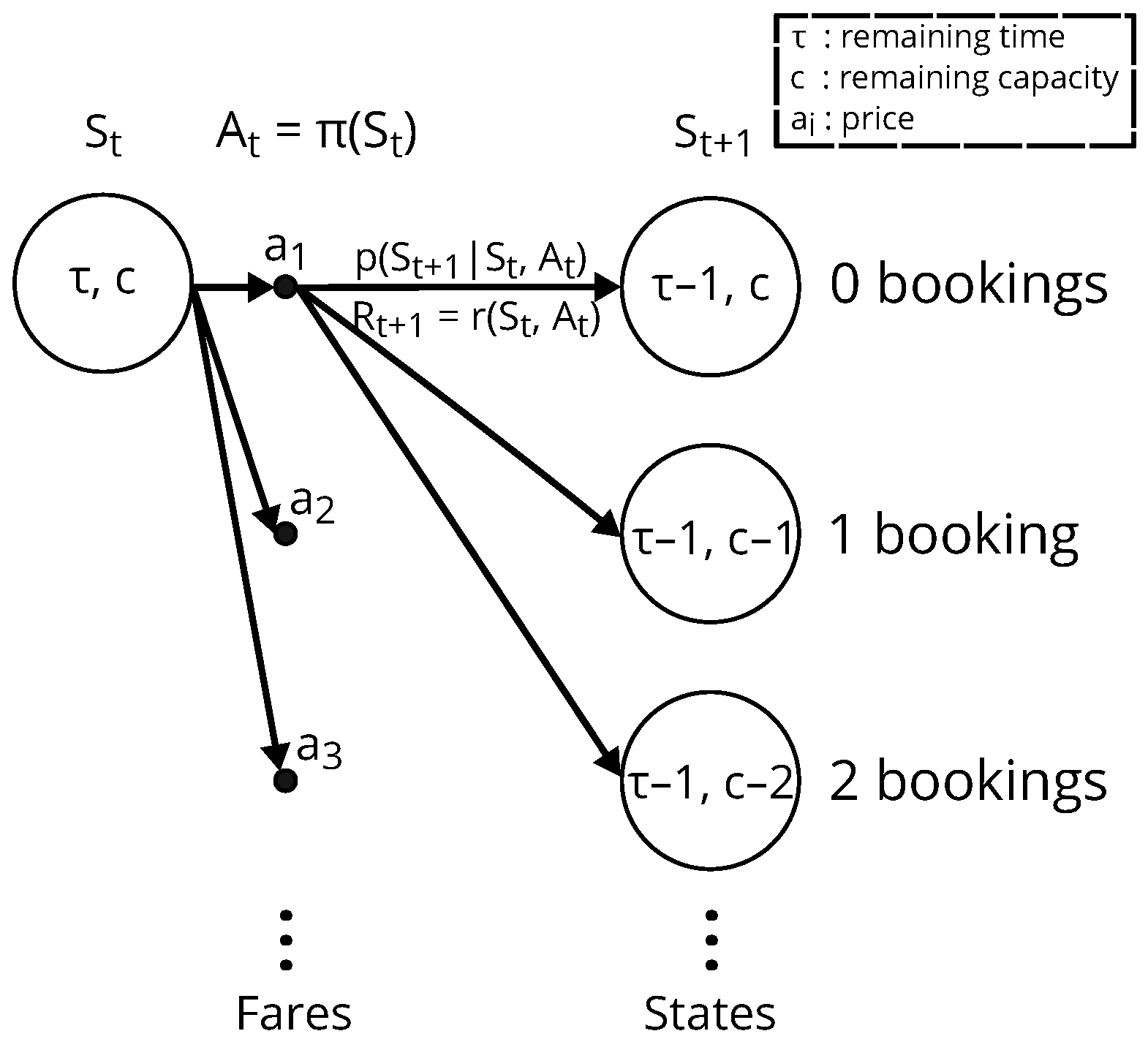
For each active flight, the pricing optimization is modeled and solved as a finite Markov decision process (MDP) [44], which is defined by a tuple , where is the state space, is the action space, is the reward function, and is the transition probability function. At each time step t (e.g., day), the RMS observes the inventory state of an active flight , denoted by the tuple , where is the number of time steps to departure, and c is the flight’s remaining capacity. Then, it takes an action (i.e., it selects a fare) according to its pricing policy . Multiple customers can arrive and interact with the RMS by choosing whether to book or not at the selected action . At the time step , with probability , the remaining capacity c decreases by the number of bookings made at the previous time step. Finally, the RMS receives a reward equal to the immediate expected revenue given by
Interactions with customers continue until the flight departs, at which point no further action can be taken, and the flight reaches the terminal state . The MDP is illustrated in Figure 2.

Figure 2.
Backup diagram for optimization of a flight.
Once the parameters of the demand model are obtained, the system needs to search for the policy that maximizes the expected return , where the return is defined as . The parameter is called the discount rate, and it defines how farsighted the system is with respect to the revenue maximization (in the case of the airline’s RM; the discount rate is very often chosen to be [14,42], because the MDP has no loops, and the episode’s horizon is finite, thus guaranteeing that the return is a finite quantity). The optimal policy according to the demand model defined by can be computed through finite-state dynamic programming (DP) methods, where we first solve the action value function by making use of the Bellman optimality equation after setting the boundary condition ,
Finally, the pricing policy for the flight is obtained by computing . In principle, this optimization procedure must be replicated for each active flight; however, given the simplicity of the assumed demand model (no seasonality nor day of week variation), the same policy function can be used across all active flights.
3.2. Reinforcement Learning
RL also uses the same underlying concepts behind DP to optimize MDPs. The RL agent’s goal is to find the policy that maps the observed state s to actions that maximize the expected return, and the procedure very often involves the computation of value functions. In contrast to DP, RL methods have strong emphasis on learning through the interaction with an environment. RL methods have mainly two important advantages over DP methods that we will exploit [7]. The first one is that they do not require an explicit distribution model, such as the one defined by , that describes every possible outcome weighted by their probabilities when transitioning from one state to another. Instead, RL methods use a sample model, that produces just one example from all possible outcomes. In many applications, sample models are often much easier to obtain, particularly when the number of possible outcomes is very large, and/or the computation of the probability of each outcome is complex. Secondly, RL does not suffer from the curse of dimensionality that occurs when the state–action space of a problem is so large that computing for all the state–action pairs becomes intractable. Alternatively, RL generates trajectories in the state–action space, and it performs updates at the pairs encountered along the way, directing the learning towards the pairs that occur more frequently, thus focusing computational resources where they are most currently needed to succeed in the task.
There are many classes of RL algorithms, but we focus on the important class of actor–critic methods. Generally, these methods seek to compute the stochastic policy function , also known as the actor, which returns the probability of selecting action a given state s, and the value function , also called the critic, which outputs the expected return from state s while following policy . In practice, the actor–critic methods usually model these two functions by the parameterized policy and parameterized value function . The main idea behind actor–critic is to perform updates for parameters to maximize the performance metric while following the policy gradient in a stochastic gradient ascent manner:
The most used policy gradient estimator has the following form (see policy gradient theorem [7] for details)
where indicates the empirical average over a finite batch of samples while following policy . The parameters for the value function can be updated according to
which can be computed through stochastic gradient descent. The actor–critic framework provides a wide range of RL algorithms (e.g., deep deterministic policy gradient [45], asynchronous advantage actor–critic [46], trust region policy optimization [47], proximal policy optimization [48], etc.), each having their respective pros and cons. In principle, for our work, any of these algorithms could be used.
Later, we present the EWL problem in its continuing nature, that is, the task of balancing between earning and learning never finishes, because, for every day, new booking data are added to the historical database and old data are deleted. For tasks with such a continuing nature (when the episode length ), we cannot choose the discount rate to be one (), because the agent’s goal, which is maximizing the expected return, would diverge [7]. Thus, choosing the discount rate may be a difficult task. If too large, learning can be unstable, whereas, if too small, the agent can be too shortsighted, preferring short-term reward to long-term goals. To overcome this limitation, an alternative classical setting for formulating the goal in MDPs, called the average reward [7], defines the quality of a policy as the average rate of reward while following that policy, denoted by
The value function is then defined in terms of the differential return:
There are several methods for computing the differential return [49], and it has been already successfully extended to the actor–critic framework [50].
4. Revisiting Earning While Learning through Reinforcement Learning
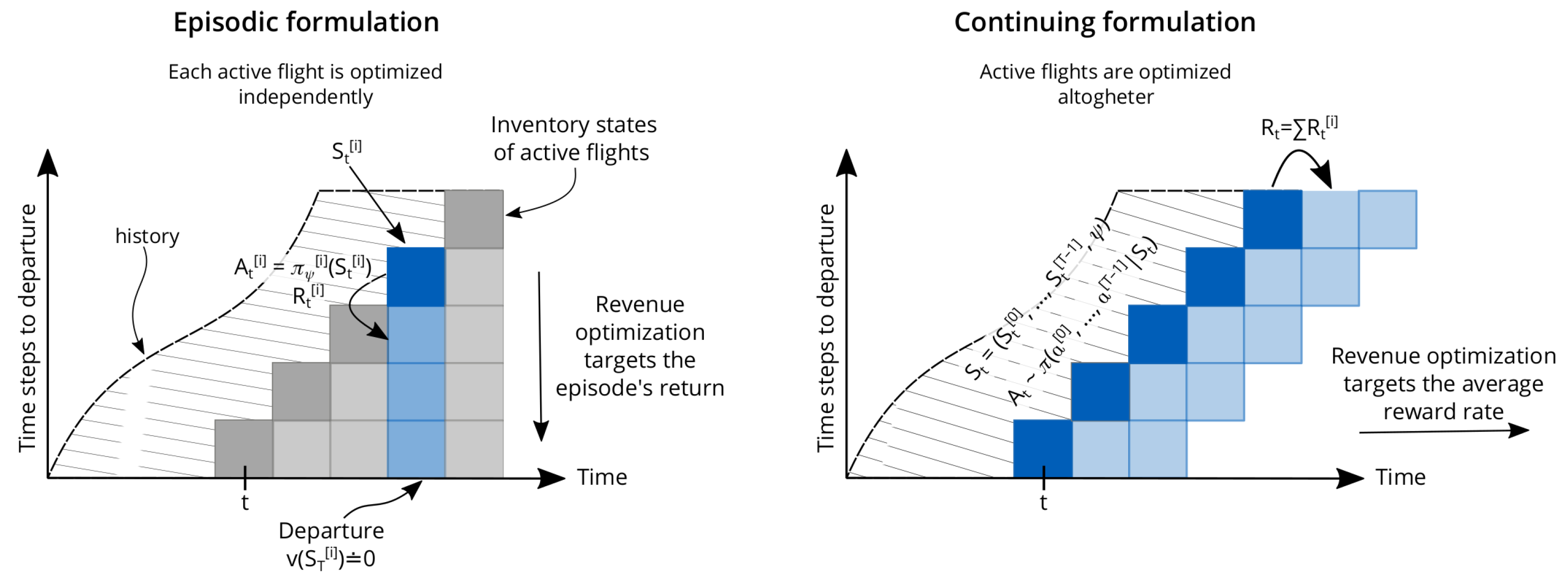
To solve the single-leg problem, the standard approach followed by legacy RMSs breaks down the problem of optimizing active flights into smaller optimization problems, each flight being optimized with DP as described in Section 3, by making use of Equation (2), as illustrated in Figure 3 (left). This approach would be correct if each flight was truly independent of the others. However, the data collected for each flight are aggregated and used for model calibration, which in turn is used for optimization in future time steps. Thus, the pricing decision of each flight has longstanding consequences for the quality of future model calibration that goes beyond the flight’s departure. Furthermore, each price decision contributes to the quality of the estimation of future demand models, making each decision a small part of a whole, suggesting that some collaboration across flights may be needed. In fact, the policy collecting data in legacy RMSs is rather a result of a set of uncoordinated policies, each seeking to maximize its own revenue independently.
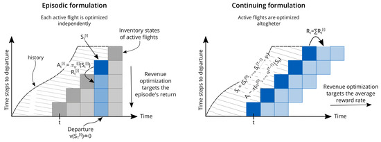
Figure 3.
Comparison between episodic and continuing formulations for revenue maximization.
To address this problem, we want to give the agent the ability to specify a unified policy that can coordinate pricing decisions across flights and that maximizes revenue beyond individual flights. Therefore, we propose to compute a policy that outputs the price decisions across the active flights altogether as illustrated in Figure 3 (right). We denote the i-th active flight on the selling horizon with superscript , such that implies the inventory state at time step t for the i-th active flight on the selling horizon. The agent’s action is a tuple containing the selected fare for each one of the active flights, i.e., . Similarly, the observation space is defined as the tuple of the inventory state for each one of the active flights and the current estimated model parameters, i.e., . A natural consequence of this choice is that we need to redefine the reward signal as the sum of the immediate revenue obtained for each one of the active flights, i.e., , addressing the second point of maximizing the combined revenue across all flights.
Our goal is to find the pricing policy that maximizes the combined revenue. Note that the dimensionality of the problem makes it impossible to solve it with exact methods such as DP. The cardinality of the action space alone is , which makes it impractical even for toy problems. The observation space has a discrete component with size and a continuous component representing the estimated model parameters . The transition probabilities, which we enumerate in Section 3.1, is now one set too large () to be computed exactly. These characteristics make this problem very appealing to address with RL, because RL approximates the policy and value functions, enabling us to represent large state–action spaces, and it uses a simple and cheap sample model to perform trajectory sampling, in contrast to the expensive computation of the transition probabilities required by DP.
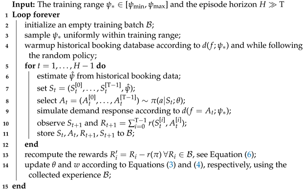
Among the many RL methods in literature, algorithms that use policy parameterization, such as actor–critic methods, are well suited to large action spaces [51]. In Algorithm 1, we present the training pseudocode of the actor–critic framework to the EWL problem. We compute a parameterized policy and a parameterized value function as usual (see Section 3.2). The training environment uses a sample model, where each active flight interacts with a simulated demand following the ordinary assumptions (Poisson arrivals, negative exponential purchase probability), and the estimation of the demand model parameters is also performed also as usual [33,43]. Perhaps the only difference from the standard methods is how the total return is computed. When we redefined the state–action space and the reward signal to contain the aggregation of the state and rewards for all active flights, the “episodic” concepts of the starting and terminal states from Section 3.1 disappeared with it. At each time step, the RL agent observes the sequence of the inventory states and the latest model parameters, and it selects the fares for each active flight. This continues from any particular starting point without termination. The continuing nature of the task suggests the use of the average reward defined in Equation (5).
| Algorithm 1: Actor–critic for EWL. |
 |
The way the EWL problem is formulated for the RL agent is related to multitask reinforcement learning (each set of true demand parameters define a new transition probabilities and thus to a new task) and partial observability (the true demand parameters are unknown to the system). The RL agent is not informed which task it is solving, and it needs to discover which task it is solving along the way through the unreliable estimated demand parameters. In fact, we borrow some ideas from these fields, such as the use of universal function approximators (inputs of the value function) [52], and the use of a (supervised) state-estimator function (which corresponds to the forecasting module that computes the estimated model parameters) [53].
With regard to the modeling of the policy and the value functions in Algorithm 1, we suggest the use of artificial neural networks. We recognize that there may be many possible designs for the artificial neural network (ANN), and finding the best one is not the focus of our work. We find that the architecture illustrated in Figure 4, which uses a long short-term memory (LSTM) [54], the Luong-style attention mechanism [55] following the encoder–decoder architecture [56], delivers stable training and good performance results. Perhaps the most important aspect of our design is the use of the LSTM decoder in the actor network. The number of output units grows linearly with respect to the number of parallel active flights (i.e., for each active flight, the agent must compute the probability of selecting each fare in the fare structure), and it can quickly cause the ANN to have too many outputs to learn. By using an LSTM decoder, the ANN can share the learned parameters between the outputs of each active flight, allowing a more compact and efficient representation.
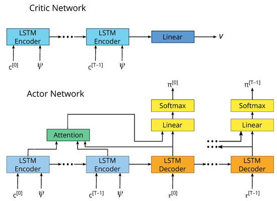
Figure 4.
The artificial neural network architecture consists of two separate networks. The critic network approximates the value function, and the actor network approximates the policy function. The long short-term memory (LSTM) encoder takes the remaining capacity inputs , and the LSTM decoder takes the remaining time inputs , and it outputs the probability of selecting each fare in the fare structure for each active flight.
5. Experiments
We separate our experiments into two distinct scenarios. In the first one, we compare the RL agent to the heuristic method defined in Equation (1) while estimating a single demand-model parameter (price sensitivity ). The heuristic method can be adapted to the single-leg problem under the assumption of unconstrained capacity (i.e., infinite inventory capacity) [33]. Even though the unconstrained capacity is an unrealistic assumption for most real-world scenarios in airline RMs, this experiment provides a baseline to measure the effectiveness of the RL agent when solving the EWL in the single-leg problem. In the second, we compare the solution obtained by RL with the standard RMS (which behaves as certainty equivalent pricing, as described in Section 2) when capacity is constrained, and we assume the system must estimate two model parameters from historical booking data (arrival rate , and price sensitivity ). This scenario aims to demonstrate that our method can learn how to solve more complex settings (such as controlling the uncertainty over two model parameters), and that it can also learn how to optimize pricing under capacity constraints (which is not possible with the work developed in [33]).
Throughout the experiments, we assume that each flight has the capacity (representing, for example, the number of seats in the business cabin), the fare structure has 10 price points , the booking horizon has time steps, the demand follows the exponential model, and the historical database keeps the booking data for the most recent flights. Furthermore, we refer to the price sensitivity in terms of the fare ratio of the lowest fare at which the purchase probability is 50% [57], abbreviated as frat5, which is defined as
The frat5 greatly simplifies interpretation, because it has a linear relationship to revenue-maximizing fare under the assumption of the exponential demand model.
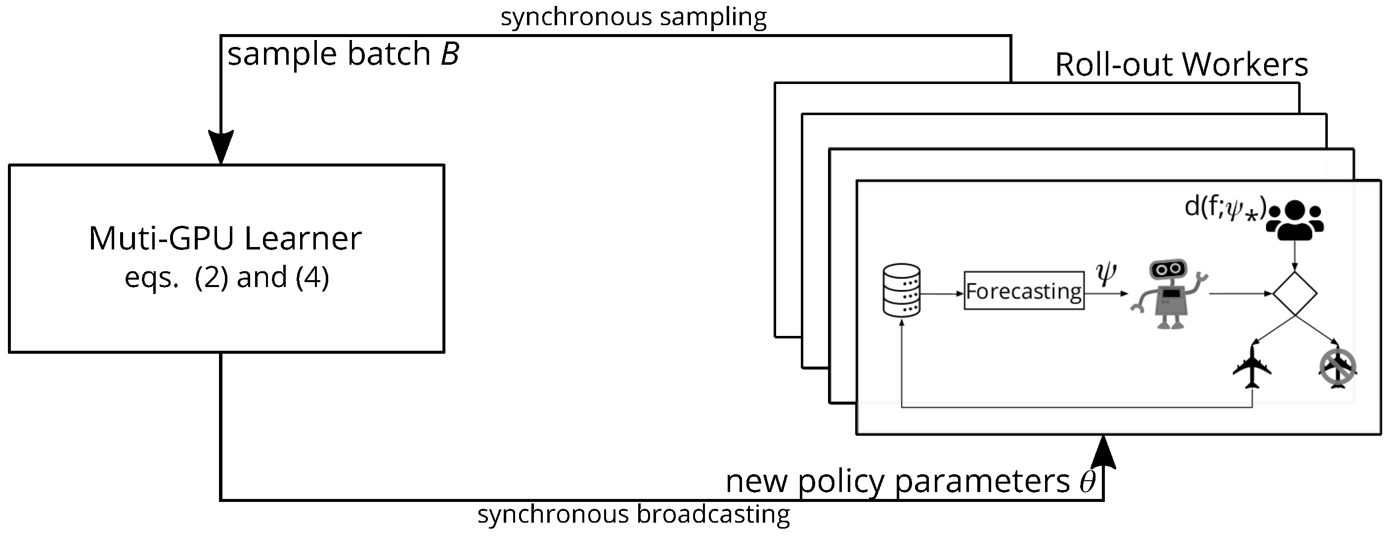
As illustrated in Figure 5, for the RL training set up we use the proximal policy optimization algorithm (PPO) [48] because of its simplicity and stability, and we use RLLib [58] to distribute training computation in a cluster with 4 GPUs and 24 CPUs. The training hyperparameters set for the PPO algorithm for the two investigated scenarios can be found in Table 2.
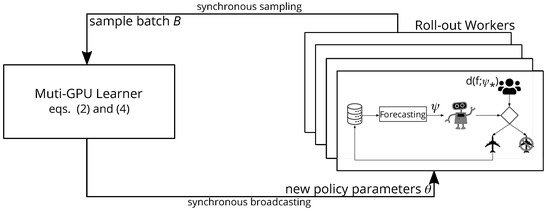
Figure 5.
The proximal policy optimization algorithm training architecture for earning while learning. A copy of actor network is deployed to each roll-out worker responsible for generating training experience according to the true demand behavior specified by . The agent cannot observe the true demand behavior parameters directly, and its decisions rely on exclusively the estimated demand behavior parameters instead. The training experience generated by all roll-out workers are aggregated into a batch and then sent to the learner which is responsible for updating the neural networks weights.

Table 2.
Training hyperparameters. “ep.” abbreviates episode. The RLLib implementation of PPO dedicates one CPU to the master thread, which is not used for generating experience.
5.1. Estimating Only the Price Sensitivity under Unconstrained Capacity
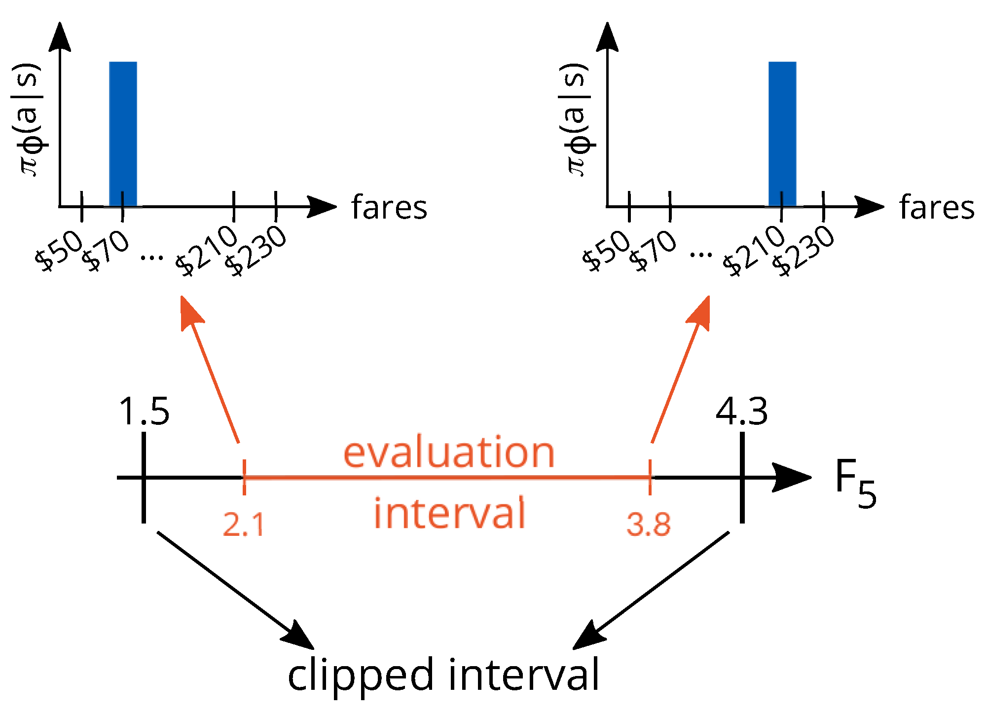
In this section, we follow the experimental settings proposed in [33]. We consider the case where the system must estimate only the price sensitivity parameter , and that the true arrival rate is fixed and known at all time steps (no estimation of this parameter is needed). We evaluate the methods under a low number of arrivals, because the scarcity of booking data for estimating the demand price sensitivity makes the problem very challenging, being efficient price experimentation essential to success in the task. Even though the capacity is finite, , given the very low arrival rate , it is extremely unlikely that the flight’s capacity will ever exhaust even if the lowest fare (the fare for which purchase probability is one) is selected at all time steps (). Therefore, from the optimization perspective, the capacity is practically infinite, allowing us to implement the heuristic method as presented in [33]. Moreover, we perform model calibration at every time step, and we evaluate both the heuristic method from [33] and RL within the interval . In this interval, the revenue-maximizing fare if the true demand behavior were known covers almost the entirety of the fare structure. In theory, the system does not know anything about the evaluation interval, and any positive value of the price sensitivity could be assumed. However, to avoid extreme evaluations for the price sensitivity parameter, we limit its estimates to be within the range (this parameter clipping applies to all methods: RL, RMS, and heuristic). Safety mechanisms such as this one are often present in real-world systems. In Figure 6, we illustrate the relationship of these two intervals with the revenue-maximizing policy when the true price sensitivity of the demand is known by the system at all time steps.

Figure 6.
An illustration of the clipped and evaluation intervals and their corresponding revenue-maximizing policies.
Algorithm 1 requires two inputs. The first input is the value that the model parameters may assume. Given our settings, we have two natural choices: we can either choose to train under the evaluation interval or under the “clipped” interval. We choose the clipped interval (), because the two most extreme price points are never optimal in the evaluation interval, and RL could easily learn how to exploit this fact. For example, if the estimation of the price sensitivity parameter is too unreliable to be useful, RL could still learn that the most extreme price points should never be chosen (as illustrated in Figure 6), whereas the heuristic methods would require to be informed of this fact explicitly. One could argue that this is an advantage, but we believe that the comparison is fairer between heuristic and RL if the agent cannot know the true range of the evaluation interval during training. With respect to the second input, the episode horizon, we can choose any arbitrary value larger than the booking horizon . If this value is too small, the agent might never actually observe the long-term consequences of its choices. We find that time steps is appropriate for our goals.
We focus our analysis on the revenue performance, represented by the average collected revenue normalized with respect to the revenue-maximizing policy (which knows the true demand price sensitivity at every time step) and the random policy (that selects fares from a uniformly random distribution). Furthermore, we also look at the mean square error (MSE) of the estimated price sensitivity (representing the demand model quality), which is given by
where is a sample estimation of the price sensitivity. We perform each evaluation run following the same training procedure from in Algorithm 1, that is, first we set the true demand behavior parameters, then we warm up the historical database using the random policy, and finally we roll out each method’s policy for 440 steps (the computation of the average reward and the update of the neural network weights are not performed during the evaluation). In contrast to the training algorithm, we discard the first time steps of data, because we want to compare each method in its stable regime.
We separate the analysis into two distinct parts. In the first part, we compare how each method behaves within the evaluation interval, then we perform a more detailed analysis of the final pricing policy obtained for each method.
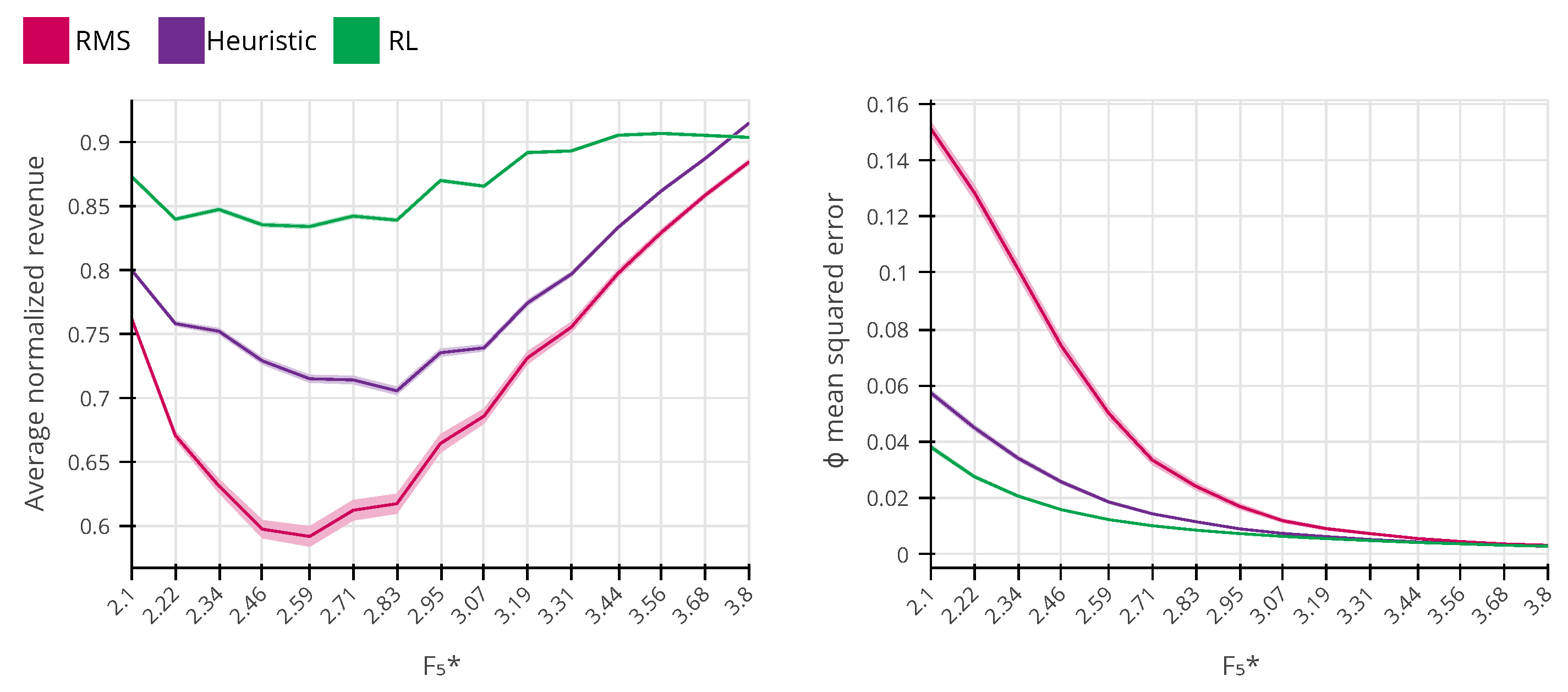
In Figure 7, we set the true frat5 parameter to the fixed values of the evaluation interval, and, for each frat5, we compute the average revenue performance and the price sensitivity MSE for 3565 independent evaluation runs. For the heuristic method, we choose a constant value for the trade-off parameter (see Equation (1)), which is the value that maximizes the expected revenue for the evaluation interval. In Figure 7 (left), we observe that RL outperforms both RMS and the heuristic method in the entire interval, except for . The reason why RL does not perform as well as the heuristic method for will be explained in the second experiment of this section, when we illustrate the final policy obtained for both methods. In Figure 7 (right), we plot the MSE over the estimation of the price sensitivity. We see that all methods have larger values for price sensitivity MSE for lower values of frat5, which decreases as the frat5 increases. The same effect is observed and explained in [33]. In short, this is because the true arrival rate parameter is known by the system. As the frat5 increases, so does the optimal fare, and the higher the selected price is, the more information is obtained about the customers’ price sensitivity. Moreover, we see that RL also produces lower price sensitivity MSE than the RMS and the heuristic method. The RL agent pricing policy displays a better estimation of the demand price sensitivity, and it also generates more revenue on average than the heuristic method and RMS.
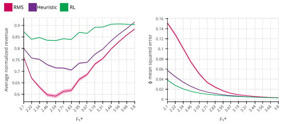
Figure 7.
The comparison between the average performance of the revenue management system (RMS), the heuristic method from [33] and reinforcement learning (RL) (99% confidence level). The system’s performance is better the higher the average normalized revenue is (the best theoretical response that requires the perfect knowledge of the demand parameters of all time steps is normalized to be one). On the right chart, we show the estimation mean squared error of demand model, which indicates that smaller errors are better.
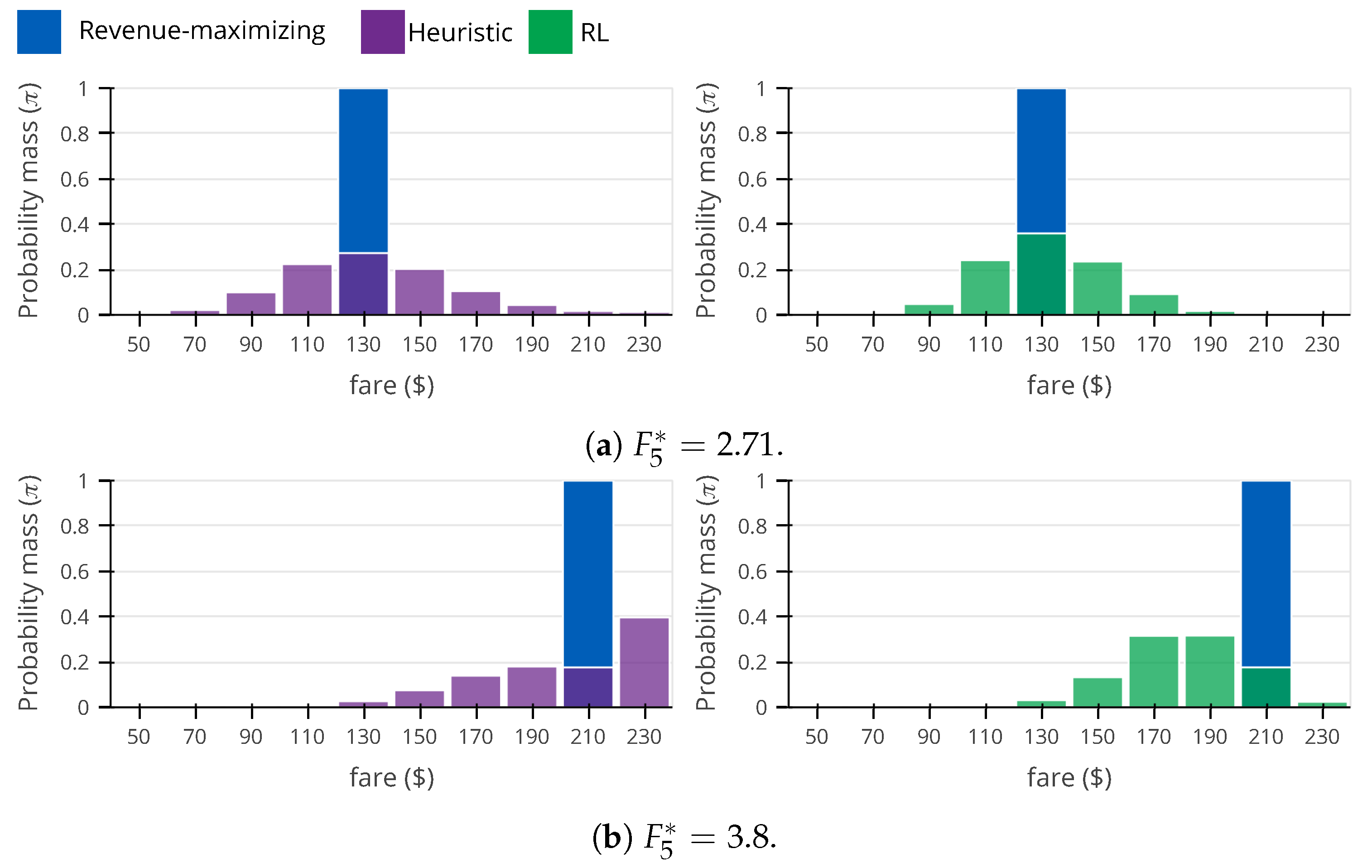
In Figure 8, we show the pricing policy obtained through Monte-Carlo roll-outs for both heuristic and RL methods. When true frat5 (Figure 8a), RL shows a large performance advantage with respect to the heuristic method (see Figure 7) and also a smaller price sensitivity MSE. The reason is clear when comparing the two policies. RL tends to price closer to the true optimal fare, that is, it prices fares $110, $130, and $150 more frequently (83.6%) than the heuristic method (69.9%). RL is also slightly more efficient than the heuristic method with respect to the price sensitivity MSE, because RL tends to price the higher fares more frequently (70.7%) than the heuristic method (65.1%) (in this problem setting, higher fares contain more information about the demand price sensitivity than the lower fares). When true frat5 (Figure 8b), RL generates less revenue than the heuristic method, and they both display the same price sensitivity MSE. Analyzing the heuristic and RL policies closely, we see that the largest difference is that the heuristic method selects the highest fare $230 often (39.6%), while RL rarely selects the same fare (2.4%). This is very surprising, because, under the evaluation settings, the highest fare is near optimal for revenue maximization and also near optimal for the estimation of the demand price sensitivity (see eq. (2) from [33]). The reason the fare $230 is preferred by the heuristic is because, at frat5 , price sensitivity clipping happens frequently (20.1%; same number is observed with RL), causing the heuristic algorithm to select the fare of $230. When the price sensitivity parameter is clipped (and the estimated uncertainty of the price sensitivity is unavailable), it is impossible for the system to know whether it was clipped due to large errors or if it was clipped because the true value is close to the limits. Compared to the heuristic (which has access to the estimation of the price sensitivity uncertainty, see Equation (1)), RL takes a more conservative approach, distrusting the parameter estimation and pricing fares ($170, $190 and $210) that are often better for the estimation of the demand price sensitivity and that work well for high values of frat5.
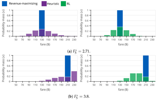
Figure 8.
Comparison between heuristic and reinforcement learning (RL) roll-out policies. For convenience, we represent the revenue-maximizing policy.
5.2. Estimating the Price Sensitivity and Arrival Rate under Constrained Capacity
For our second experimental setting, we consider that the systems must estimate both demand model parameters, i.e., the arrival rate and the price sensitivity , from historical bookings. The true arrival rate can assume any value in the range , making the flights’ capacity finite in practice. As in the previous experiment, we consider that the true price sensitivity can assume any value in the range . For the same reasons as in the previous experimental setting, we train the RL agent over a clipped interval that is larger than the evaluation interval ( and ).
As in the previous section, we first analyze how the RMS and the RL agent perform in the evaluation interval with respect to revenue performance and model quality. Then, we compare how the two policies differ for a specific value of true demand behavior parameters.
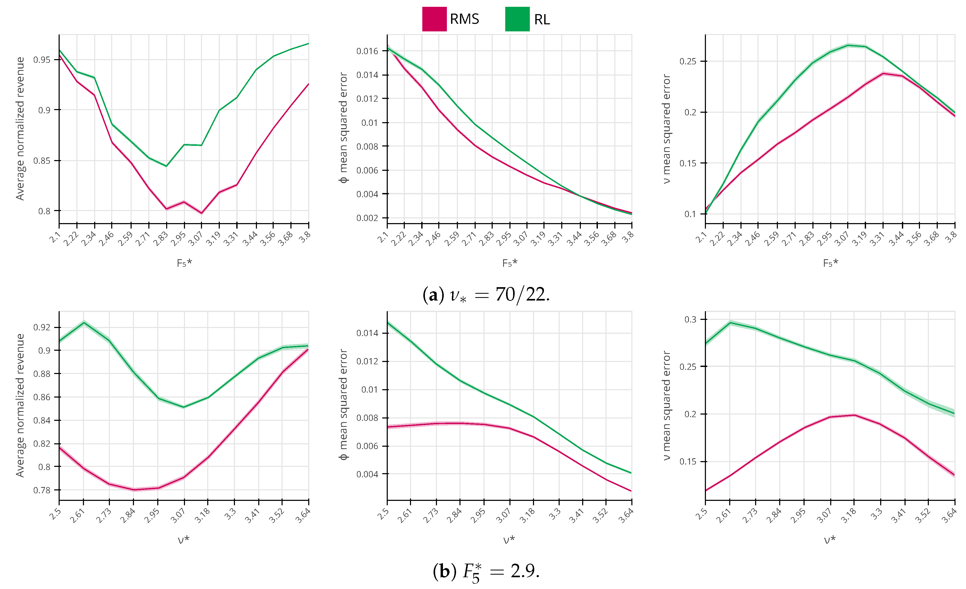
In Figure 9a, we can see how the average normalized revenue and the MSE for the demand model parameters respond to different values of true price sensitivity within the evaluation interval. From the left chart, we can see that RL outperforms RMS in the entire interval, with a larger advantage occurring with higher values of frat5. In the center and right charts, we see that the MSE errors for both parameters are close to each other, but RL consistently demonstrates a worse MSE performance. The same behavior is also present when the true customer price sensitivity is fixed, and we only vary the arrival rate, as in Figure 9b. This may seem paradoxical: how can RL perform better from the revenue maximization perspective while having a worse estimation of the demand model parameters? Unfortunately, we do not have a complete understanding of RL strategy to precisely answer this question, thus we can only speculate about its strategy. As we observe in the following analysis, instead of reducing model uncertainty, the agent can learn to select the “safe price” which it is certain will not lose too much revenue, especially when the estimated demand model parameters are found to be too extreme (i.e., close to the clipping limits).

Figure 9.
The comparison between the average performance of the revenue management system, reinforcement learning, and revenue-maximizing policies (99% confidence level).
For the second analysis, in Figure 10, we display the RMS and the RL agent pricing policies when the true arrival rate and price sensitivity are fixed at and . We choose this point because the flights’ average load factor is 70%, which brings a natural price variability and a high amount of booking data to estimate the demand model parameters (the historical data contains an average of 1078 bookings). Given these two properties, obtaining a good estimation of the demand model parameters is relatively easy for the RMS, which puts in question the value of price experimentation. The RMS achieves a normalized revenue performance of 80.6%, with an MSE for a price sensitivity and an arrival rate of 0.007 and 0.20, respectively. The agent is better for revenue maximization, with a normalized revenue performance of 89.9%, but it has a worse model quality with an MSE for a price sensitivity and an arrival rate of 0.008 and 0.26, respectively. When comparing the two policies, we see that the major difference is that the agent prefers to price center fares $130, $150, and $170 more frequently (72.1%) than the RMS (65.3%). This strategy has a negative impact on the overall model quality, because it decreases the price variability in the historical data, but it turns out that center fares are better for revenue maximization than higher fares such as $210 and $230, because they are a less extreme given the true demand behavior. This aligns with our intuition that the RL agent tends to prefer “safer prices” when “price experimentation” is less suitable.

Figure 10.
Comparison between revenue management system (RMS) (left) and reinforcement learning (RL) (right) roll out policies for , . The reinforcement learning policy performs better (89.9%) than the revenue management system policy (80.6%) with respect to the revenue performance but has worse mean squared errors for both demand model parameters.
In Table 3, we present a summary of the performance of each method for the two investigated scenarios. The results represented in the table correspond to the average behavior of 3565 episodes for each method in the evaluation range.

Table 3.
Summary of experimental results.
6. Discussion
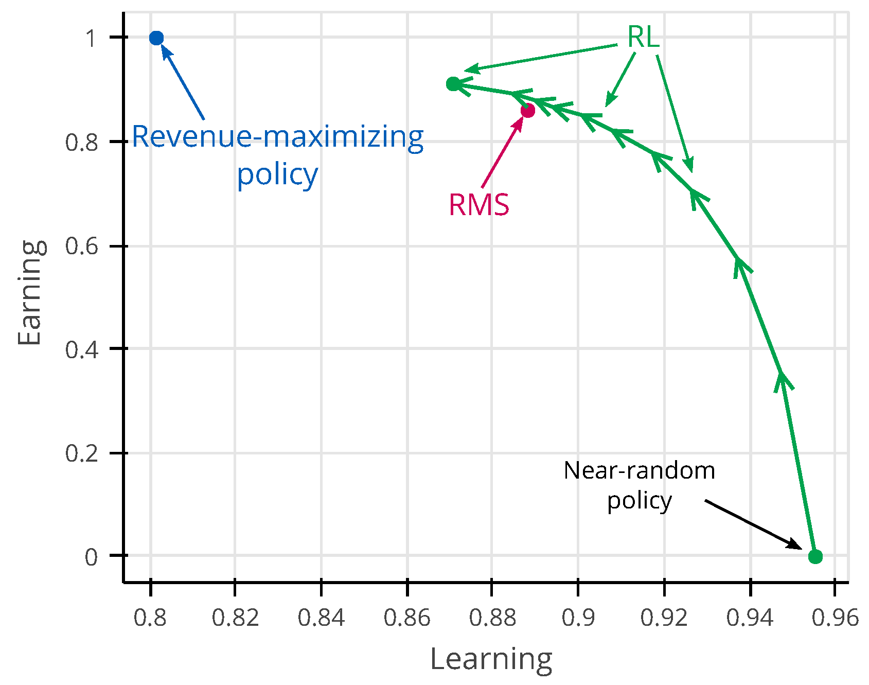
Perhaps one of the most important keys to the success of RL was the simplification the dual optimization aspect of the EWL problem into a single optimization dimension, which is the revenue maximization. Instead of describing the EWL problem as an explicit requirement of balancing revenue maximization and model learning common to heuristic methods [2,3,33], we ask the RL agent to maximize only revenue, and RL has the flexibility to trade-off between earning and learning as it finds best suitable. In Figure 11, we show how RL trades earning and learning throughout its training. This figure is computed according the same experimental settings which the RMS must use to estimate both arrival rate and price sensitivity, and the true demand behavior parameters are sampled uniformly in the evaluation interval. Prior to the start of training, RL starts following a near-random policy at the bottom right, and, as training progresses, RL policy improves its revenue performance (earning) at the expense of the demand behavior parameter’s accuracy (learning). At some point in training, RL displays the same revenue performance of RMS while presenting a better estimation of the demand model parameters. As training continues, RL is able to further improve revenue by sacrificing the demand model quality, ultimately converging towards the point of equilibrium represented by the dot at the end of its trajectory, where it cannot further improve revenue.

Figure 11.
RL trajectory in the earning–learning space. The earning axis represents the average normalized revenue for the evaluation interval, while the learning axis represents the average estimated demand parameter’s accuracy . The revenue-maximizing policy is obtained by providing the true demand behavior parameters to the optimizer while keeping the estimation of parameters of the demand model as usual. The balance found by the revenue-maximizing policy is unstable, thus not being an answer to the problem.
Since controlling model uncertainty is required to succeed in the task, we leave the mission of identifying when and how much price experimentation should be conducted to the agent. Such an approach has strong connections to the “reward is enough” hypothesis [13], which states that any associate abilities of intelligence (e.g., social intelligence, perception, knowledge representation, planning, etc.) can be understood as sub-serving the maximization of reward (i.e., the measure of success in the task). In our case, we claim that controlling the quality of the estimated demand model is the associated ability needed by the agent to achieve the maximization of reward (or revenue). We trust RL to find out the solution to all the complexities of the EWL problem from nothing more than the standard RMS raw inputs, without any human guidance.
Even though we did not investigate how our method behaves in the face of market shocks, we believe that the adaptation should be straightforward. In principle, to train the agent to react to market shocks, we can simply introduce simulated examples of market shocks by making the true demand behavior parameters a function of time in the inner loop of Algorithm 1. Indeed, this illustrates how human experts can interact with the agent in the offline setting; the expert’s mission is to define what task they want the agent to solve (in this example, the expert specifies the functional form of a market shock).
Last but not least, our method also displays some practical benefits when compared to heuristic methods such as in [33]. The RL agent has no need for any external indication of the level trust of the estimated demand model parameters (represented by the estimation of demand model uncertainty in heuristic methods). The advantage of not requiring a measure of uncertainty is that, for realistic-sized demand models that have many parameters to be calibrated, computing these quantities and balancing their importance in the optimization heuristic may not be so a trivial task. Furthermore, training the RL agent imposes a different set of constraints, such as computation requirements and fine-tuning the algorithm’s hyperparameters, which may be easier to address and less time consuming than heuristic-based methods that often require significant expert time to develop, implement, and calibrate.
7. Conclusions and Future Work
In recent years, the EWL problem has attracted attention from academia and industry, in particular since the COVID-19 pandemic, which significantly impacted the global economy, especially the airline industry. We believe that recovery requires effective price experimentation to learn the new and potentially evolving demand price sensitivity. In this work, we investigate the EWL problem in the challenging single-leg problem, where the system must control the pricing strategy of many active flights while learning the parameters of the demand model from historical bookings.
Throughout the decades, many analytical studies and heuristic methods have been proposed to address the EWL problem, with different revenue performance and implementation constraints. To the best of our knowledge, none of these methods have been successfully deployed in the airline industry yet, despite their good performance in simulation studies and real-world benchmark datasets, perhaps because of the complexity of computing the estimation of the parameter errors in realistic demand models, and the difficulty of integrating these methods with current price optimization techniques.
Inspired by recent advances in AI, we propose a novel method that does not rely on any heuristics. Instead of trying to solve the EWL problem through human design, we describe the problem to an RL agent, and we leave the agent the task of finding the solution to the problem by itself. The RL agent searches for pricing policies that maximize revenue while controlling the overall demand model quality, and the learned policies generate more revenue on average than the state-of-the-art methods. We also show that our method can be extended to more complex settings, which heuristic methods fail to address. Our results suggest that, contrary to expert intuition (expressed in most heuristic methods), “earning is enough” to solve the EWL problem; no specification of an objective balancing revenue maximization and model learning nor explicit optimization involving the uncertainty of the demand model parameters is needed.
We believe that better future solutions to the EWL problem will be found through AI improvements rather than human-designed heuristics. We suggest that RL experts should focus on investigating different ANN architectures, more adapted RL methods, enhance computation capabilities, or changes in the modeling of the observation/action space. At the same time, RM experts could concentrate on designing the training environment (the sample demand model) that the RL agent relies upon for training. Finally, we leave to the agent the task of discovering how to solve the problem, while the human designer concentrates on specifying what problem needs to be solved. We hope that our successful experience will inspire researchers to try to solve problems that rely on expert intuition through RL instead.
Author Contributions
G.G.P.: conceptualization, methodology, software, and writing. M.D.-P.: methodology, supervision, writing—review and editing. J.-C.R.: supervision, writing—review and editing. All authors have read and agreed to the published version of the manuscript.
Funding
This research was funded by Amadeus SAS and the French Industrial Agreements for Training through Research (CIFRE) program.
Institutional Review Board Statement
Not applicable.
Informed Consent Statement
Not applicable.
Data Availability Statement
Not applicable. The source code of the current work is available from the corresponding author on request.
Acknowledgments
We would like to thanks the Amadeus research team for their support during the writing of this work, in particular Thomas Fiig, Michael Wittman, Alexander Papen, and Tianshu Yang. We also would like to thank the two anonymous reviewers for their input.
Conflicts of Interest
The authors declare no conflict of interest.
References
- Fiig, T.; Weatherford, L.R.; Wittman, M.D. Can demand forecast accuracy be linked to airline revenue? J. Revenue Pricing Manag. 2019, 18, 291–305. [Google Scholar] [CrossRef]
- Den Boer, A.V.; Zwart, B. Simultaneously learning and optimizing using controlled variance pricing. Manag. Sci. 2014, 60, 770–783. [Google Scholar] [CrossRef] [Green Version]
- Elreedy, D.; Atiya, A.F.; Shaheen, S.I. Novel pricing strategies for revenue maximization and demand learning using an exploration—Exploitation framework. Soft Comput. 2021, 25, 11711–11733. [Google Scholar] [CrossRef] [PubMed]
- Keskin, N.B.; Zeevi, A. Chasing demand: Learning and earning in a changing environment. Math. Oper. Res. 2017, 42, 277–307. [Google Scholar] [CrossRef] [Green Version]
- Kumar, R.; Li, A.; Wang, W. Learning and optimizing through dynamic pricing. J. Revenue Pricing Manag. 2018, 17, 63–77. [Google Scholar] [CrossRef]
- Olsson, F. A Literature Survey of Active Machine Learning in the Context of Natural Language Processing; Swedish Institute of Computer Science: Kista, Sweden, 2009. [Google Scholar]
- Sutton, R.S.; Barto, A.G. Reinforcement Learning: An Introduction; MIT Press: Cambridge, MA, USA, 2018. [Google Scholar]
- Ferreira, K.J.; Simchi-Levi, D.; Wang, H. Online network revenue management using thompson sampling. Oper. Res. 2018, 66, 1586–1602. [Google Scholar] [CrossRef]
- Trovo, F.; Paladino, S.; Restelli, M.; Gatti, N. Multi-armed bandit for pricing. In Proceedings of the 12th European Workshop on Reinforcement Learning, Lille, France, 10–11 July 2015; pp. 1–9. [Google Scholar]
- Degrave, J.; Felici, F.; Buchli, J.; Neunert, M.; Tracey, B.; Carpanese, F.; Ewalds, T.; Hafner, R.; Abdolmaleki, A.; de Las Casas, D.; et al. Magnetic control of tokamak plasmas through deep reinforcement learning. Nature 2022, 602, 414–419. [Google Scholar] [CrossRef]
- Jumper, J.; Evans, R.; Pritzel, A.; Green, T.; Figurnov, M.; Ronneberger, O.; Tunyasuvunakool, K.; Bates, R.; Žídek, A.; Potapenko, A.; et al. Highly accurate protein structure prediction with AlphaFold. Nature 2021, 596, 583–589. [Google Scholar] [CrossRef]
- Vinyals, O.; Babuschkin, I.; Czarnecki, W.M.; Mathieu, M.; Dudzik, A.; Chung, J.; Choi, D.H.; Powell, R.; Ewalds, T.; Georgiev, P.; et al. Grandmaster level in StarCraft II using multi-agent reinforcement learning. Nature 2019, 575, 350–354. [Google Scholar] [CrossRef]
- Silver, D.; Singh, S.; Precup, D.; Sutton, R.S. Reward is enough. Artif. Intell. 2021, 299, 103535. [Google Scholar] [CrossRef]
- Bondoux, N.; Nguyen, A.Q.; Fiig, T.; Acuna-Agost, R. Reinforcement learning applied to airline revenue management. J. Revenue Pricing Manag. 2020, 19, 332–348. [Google Scholar] [CrossRef]
- Kastius, A.; Schlosser, R. Dynamic pricing under competition using reinforcement learning. J. Revenue Pricing Manag. 2021, 21, 50–63. [Google Scholar] [CrossRef]
- Shihab, S.A.; Wei, P. A deep reinforcement learning approach to seat inventory control for airline revenue management. J. Revenue Pricing Manag. 2021, 21, 183–199. [Google Scholar] [CrossRef]
- Silver, D.; Schrittwieser, J.; Simonyan, K.; Antonoglou, I.; Huang, A.; Guez, A.; Hubert, T.; Baker, L.; Lai, M.; Bolton, A.; et al. Mastering the game of go without human knowledge. Nature 2017, 550, 354–359. [Google Scholar] [CrossRef]
- Hansen, B. Report of the Uppsala Meeting, August 2–4, 1954. Econometrica 1955, 23, 198–216. [Google Scholar]
- Hawkins, E.R. Methods of estimating demand. J. Mark. 1957, 21, 428–438. [Google Scholar] [CrossRef]
- Lobo, M.S.; Boyd, S. Pricing and learning with uncertain demand. In Proceedings of the INFORMS Revenue Management Conference, Honolulu, HI, USA, 2–5 June 2003. [Google Scholar]
- Chhabra, M.; Das, S. Learning the demand curve in posted-price digital goods auctions. In Proceedings of the 10th International Conference on Autonomous Agents and Multiagent Systems, Taipei, Taiwan, 2–6 May 2011; Volume 1, pp. 63–70. [Google Scholar]
- Kwon, H.D.; Lippman, S.A.; Tang, C.S. Optimal markdown pricing strategy with demand learning. Probab. Eng. Inf. Sci. 2012, 26, 77–104. [Google Scholar] [CrossRef]
- Besbes, O.; Zeevi, A. On the minimax complexity of pricing in a changing environment. Oper. Res. 2011, 59, 66–79. [Google Scholar] [CrossRef] [Green Version]
- Keskin, N.B.; Zeevi, A. Dynamic pricing with an unknown demand model: A symptotically optimal semi-myopic policies. Oper. Res. 2014, 62, 1142–1167. [Google Scholar] [CrossRef] [Green Version]
- Chen, N.; Gallego, G. Nonparametric pricing analytics with customer covariates. Oper. Res. 2021, 69, 974–984. [Google Scholar] [CrossRef]
- Chen, N.; Gallego, G. A Primal—Dual Learning Algorithm for Personalized Dynamic Pricing with an Inventory Constraint. Available online: https://pubsonline.informs.org/doi/abs/10.1287/moor.2021.1220 (accessed on 10 February 2022).
- Aoki, M. On a dual control approach to the pricing policies of a trading specialist. In Proceedings of the IFIP Technical Conference on Optimization Techniques, Rome, Italy, 7–11 May 1973; Springer: Berlin/Heidelberg, Germany, 1973; pp. 272–282. [Google Scholar]
- Chong, C.Y.; Cheng, D. Multistage pricing under uncertain demand. In Annals of Economic and Social Measurement; NBER: Cambridge, MA, USA, 1975; Volume 4, Number 2; pp. 311–323. [Google Scholar]
- McLennan, A. Price dispersion and incomplete learning in the long run. J. Econ. Dyn. Control 1984, 7, 331–347. [Google Scholar] [CrossRef]
- Rothschild, M. A two-armed bandit theory of market pricing. J. Econ. Theory 1974, 9, 185–202. [Google Scholar] [CrossRef]
- Besbes, O.; Zeevi, A. Dynamic pricing without knowing the demand function: Risk bounds and near-optimal algorithms. Oper. Res. 2009, 57, 1407–1420. [Google Scholar] [CrossRef] [Green Version]
- Den Boer, A.V.; Zwart, B. Dynamic pricing and learning with finite inventories. Oper. Res. 2015, 63, 965–978. [Google Scholar] [CrossRef] [Green Version]
- Gatti Pinheiro, G.; Defoin-Platel, M.; Regin, J.C. Optimizing revenue maximization and demand learning in airline revenue management. arXiv 2022, arXiv:2203.11065. [Google Scholar]
- Aviv, Y.; Pazgal, A. Dynamic Pricing of Short Life-Cycle Products through Active Learning; Olin School Business, Washington University: St. Louis, MO, USA, 2005. [Google Scholar]
- Cope, E. Bayesian strategies for dynamic pricing in e-commerce. Nav. Res. Logist. (NRL) 2007, 54, 265–281. [Google Scholar] [CrossRef]
- Xia, C.H.; Dube, P. Dynamic pricing in e-services under demand uncertainty. Prod. Oper. Manag. 2007, 16, 701–712. [Google Scholar] [CrossRef]
- Thompson, W.R. On the likelihood that one unknown probability exceeds another in view of the evidence of two samples. Biometrika 1933, 25, 285–294. [Google Scholar] [CrossRef]
- Auer, P.; Cesa-Bianchi, N.; Fischer, P. Finite-time analysis of the multiarmed bandit problem. Mach. Learn. 2002, 47, 235–256. [Google Scholar] [CrossRef]
- Brafman, R.I.; Tennenholtz, M. R-max-a general polynomial time algorithm for near-optimal reinforcement learning. J. Mach. Learn. Res. 2002, 3, 213–231. [Google Scholar]
- Kearns, M.; Singh, S. Near-optimal reinforcement learning in polynomial time. Mach. Learn. 2002, 49, 209–232. [Google Scholar] [CrossRef] [Green Version]
- Pathak, D.; Agrawal, P.; Efros, A.A.; Darrell, T. Curiosity-driven exploration by self-supervised prediction. In Proceedings of the International Conference on Machine Learning, Sydney, Australia, 6–11 August 2017; pp. 2778–2787. [Google Scholar]
- Gallego, G.; Van Ryzin, G. Optimal dynamic pricing of inventories with stochastic demand over finite horizons. Manag. Sci. 1994, 40, 999–1020. [Google Scholar] [CrossRef] [Green Version]
- Newman, J.P.; Ferguson, M.E.; Garrow, L.A.; Jacobs, T.L. Estimation of choice-based models using sales data from a single firm. Manuf. Serv. Oper. Manag. 2014, 16, 184–197. [Google Scholar] [CrossRef] [Green Version]
- Talluri, K.T.; Van Ryzin, G.; Van Ryzin, G. The Theory and Practice of Revenue Management; Springer: Berlin/Heidelberg, Germany, 2004; Volume 1. [Google Scholar]
- Silver, D.; Lever, G.; Heess, N.; Degris, T.; Wierstra, D.; Riedmiller, M. Deterministic policy gradient algorithms. In Proceedings of the International Conference on Machine Learning, Beijing, China, 21–26 June 2014; pp. 387–395. [Google Scholar]
- Mnih, V.; Badia, A.P.; Mirza, M.; Graves, A.; Lillicrap, T.; Harley, T.; Silver, D.; Kavukcuoglu, K. Asynchronous methods for deep reinforcement learning. In Proceedings of the International Conference on Machine Learning, New York, NY, USA, 20–22 June 2016; pp. 1928–1937. [Google Scholar]
- Schulman, J.; Levine, S.; Abbeel, P.; Jordan, M.; Moritz, P. Trust region policy optimization. In Proceedings of the International Conference on Machine Learning, Lille, France, 6–11 July 2015; pp. 1889–1897. [Google Scholar]
- Schulman, J.; Wolski, F.; Dhariwal, P.; Radford, A.; Klimov, O. Proximal policy optimization algorithms. arXiv 2017, arXiv:1707.06347. [Google Scholar]
- Wan, Y.; Naik, A.; Sutton, R.S. Learning and planning in average-reward markov decision processes. In Proceedings of the International Conference on Machine Learning, Virtual. 18–24 July 2021; pp. 10653–10662. [Google Scholar]
- Zhang, S.; Wan, Y.; Sutton, R.S.; Whiteson, S. Average-Reward Off-Policy Policy Evaluation with Function Approximation. arXiv 2021, arXiv:2101.02808. [Google Scholar]
- Degris, T.; White, M.; Sutton, R.S. Off-policy actor–critic. arXiv 2012, arXiv:1205.4839. [Google Scholar]
- Schaul, T.; Horgan, D.; Gregor, K.; Silver, D. Universal value function approximators. In Proceedings of the International Conference on Machine Learning, Lille, France, 6–11 July 2015; pp. 1312–1320. [Google Scholar]
- Kaelbling, L.P.; Littman, M.L.; Cassandra, A.R. Planning and acting in partially observable stochastic domains. Artif. Intell. 1998, 101, 99–134. [Google Scholar] [CrossRef] [Green Version]
- Hochreiter, S.; Schmidhuber, J. Long short-term memory. Neural Comput. 1997, 9, 1735–1780. [Google Scholar] [CrossRef]
- Luong, M.T.; Pham, H.; Manning, C.D. Effective approaches to attention-based neural machine translation. arXiv 2015, arXiv:1508.04025. [Google Scholar]
- Badrinarayanan, V.; Kendall, A.; Cipolla, R. Segnet: A deep convolutional encoder-decoder architecture for image segmentation. IEEE Trans. Pattern Anal. Mach. Intell. 2017, 39, 2481–2495. [Google Scholar] [CrossRef]
- Belobaba, P.P.; Hopperstad, C. Algorithms for revenue management in unrestricted fare markets. In Proceedings of the Meeting of the INFORMS Section on Revenue Management; Massachusetts Institute of Technology: Cambridge, MA, USA, 2004. [Google Scholar]
- Liang, E.; Liaw, R.; Nishihara, R.; Moritz, P.; Fox, R.; Goldberg, K.; Gonzalez, J.; Jordan, M.; Stoica, I. RLlib: Abstractions for distributed reinforcement learning. In Proceedings of the International Conference on Machine Learning, Stockholm, Sweden, 10–15 July 2018; pp. 3053–3062. [Google Scholar]
- Schulman, J.; Moritz, P.; Levine, S.; Jordan, M.; Abbeel, P. High-dimensional continuous control using generalized advantage estimation. arXiv 2015, arXiv:1506.02438. [Google Scholar]
Publisher’s Note: MDPI stays neutral with regard to jurisdictional claims in published maps and institutional affiliations. |
© 2022 by the authors. Licensee MDPI, Basel, Switzerland. This article is an open access article distributed under the terms and conditions of the Creative Commons Attribution (CC BY) license (https://creativecommons.org/licenses/by/4.0/).

