
Improved Scheduling Algorithm for Synchronous Data Flow Graphs on a Homogeneous Multi-Core Systems


Abstract
:1. Introduction
- Using data-driven thinking, the DAG computational model is extended to propose the SDAG model, which is applicable to the scheduling of dataflow programs under the current common processor architecture platforms;
- Improved the currently used SDFG scheduling algorithm to achieve better speedup;
- A new SDFG random generator was designed and used to create an SDFG dataset for evaluating the scheduling algorithm. The data are stored in matrix format, eliminating the need to create additional xml parsers and making it easier for researchers to use.
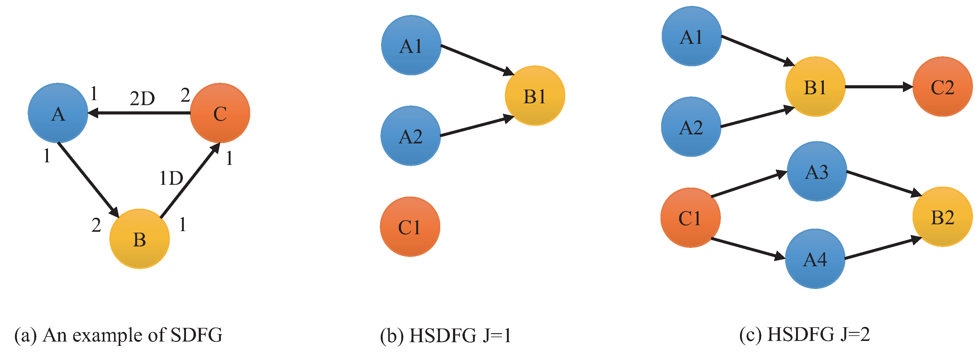
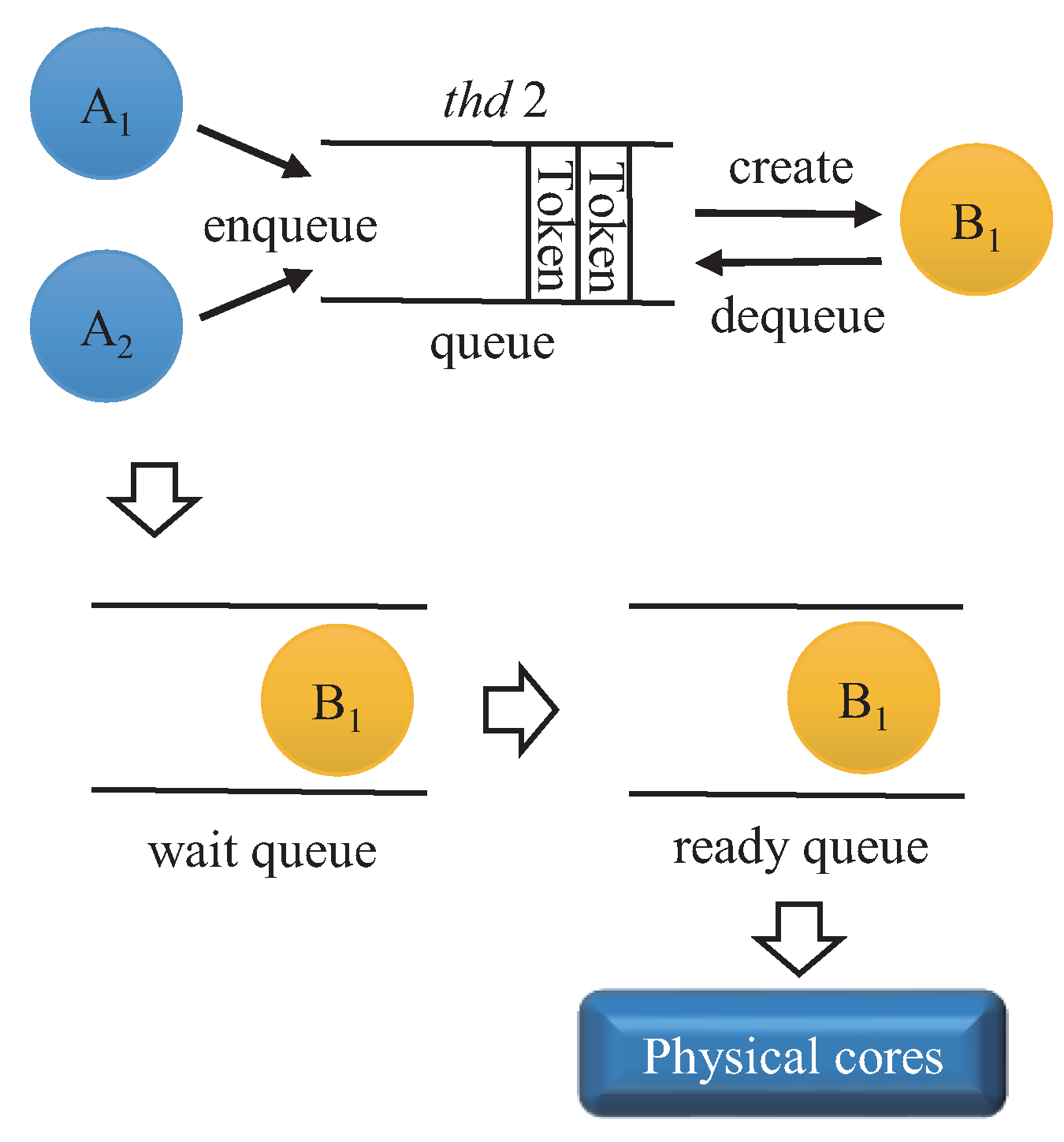
2. SDFG Background
Construction of the HSDFG Algorithm
| Algorithm 1: Constructing the HSDFG |
| Input: SDFGm Output: HSDFG 1: , , O is zero vector. 2: Iterate over the actor in the sequence 3: IF , then perform Step 2, else perform Step 4. 4: Calculate to judge whether the actor can be executed. If not, perform Step 2. If so, , and create the -th instance . Then add to the instance sequence . 5: Check whether the precursor set of the actor has elements. If not, perform Step 9. Else perform Step 6. 6: Iterate through the precursor actor set of the actor to obtain the precursor actor and the connected directed edge a. 7: Calculate d value, using . If , then . Establish a precursor relationship between the first d instances of actor and instance . 8: Update . If the current traversal is not complete, perform Step 2; else, preform Step 9. 9: For all actors, if , then algorithm is terminated. Else perform Step 2 and start a new round of traversal. |
3. Related Work
4. SDAG Model and HSDFG Scheduling
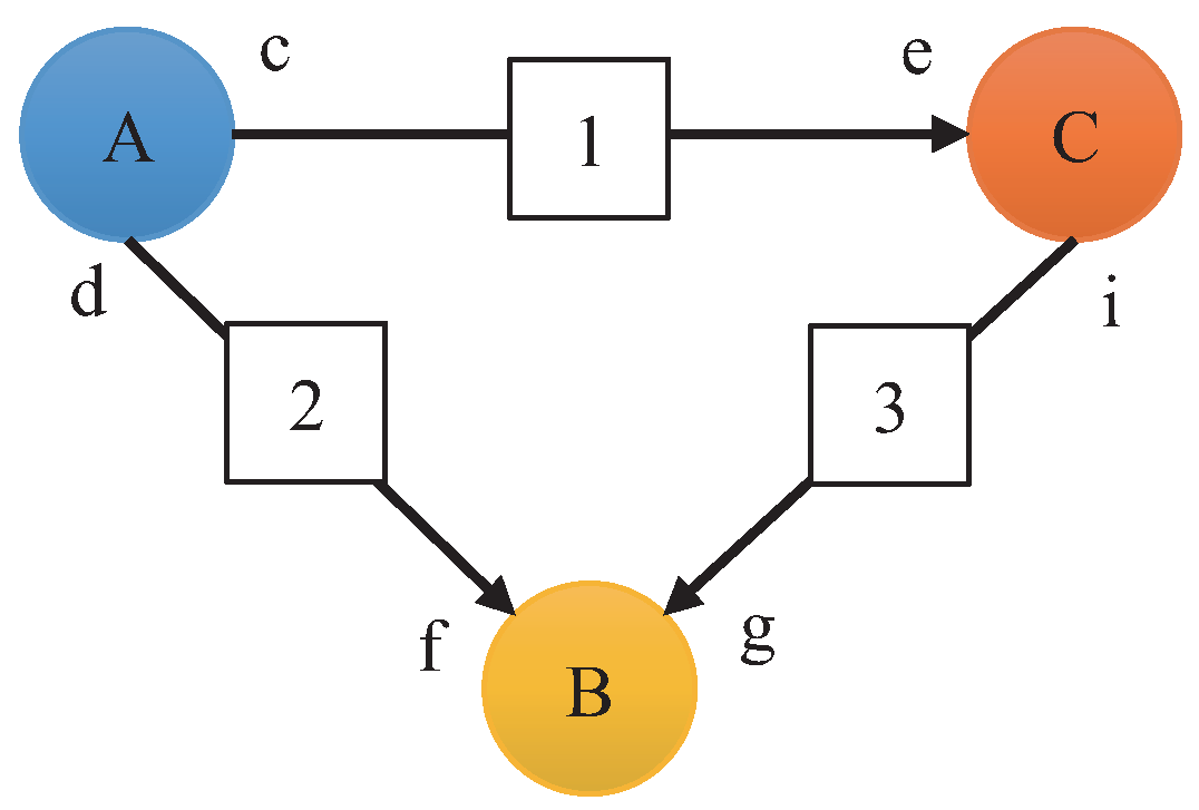
4.1. SDAG Computational Model
4.2. SDAG Computational Model Analysis
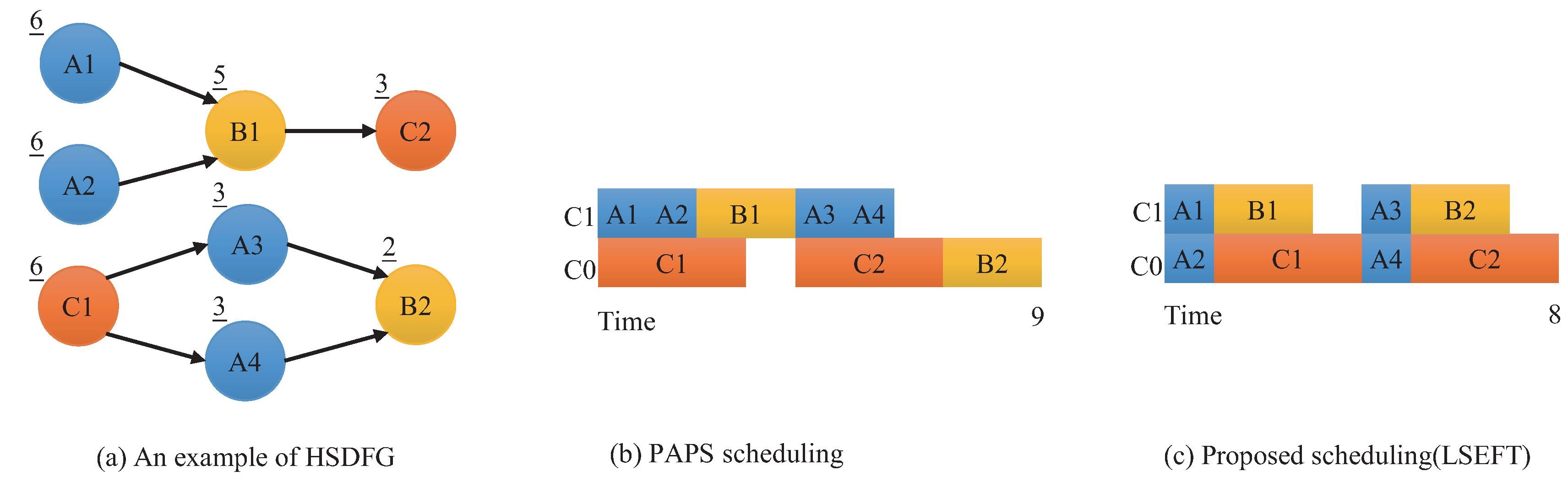
4.3. HSDFG Scheduling
4.3.1. Problem Definition
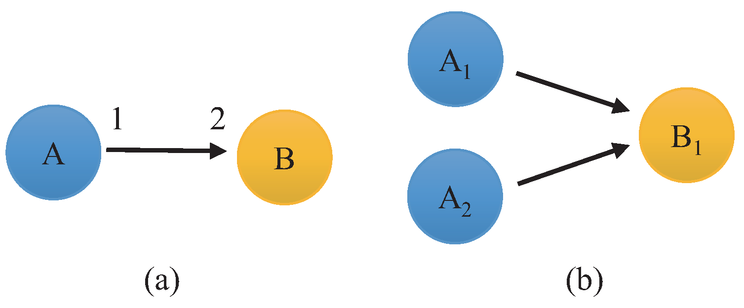
4.3.2. Instance Selection
| Algorithm 2: Calculate Level Values of Instances |
| Input: HSDFG Output: each instance level value 1: Put all instances of HSDFG are in reverse order into queue F, each instance has a set of precursor instance 2: , 3: for all do 4: for all do 5: 6: if then 7: 8: end if 9: end for 10: end for |
4.3.3. Core Selection
4.3.4. Overall Algorithm
| Algorithm 3: LSEFT Algorithm |
|
Input: queue F, set of cores M Output: scheduling result 1: Create empty queue D 2: , 3: Compute level value using Algorithm 1 4: repeat 5: Put instance with maximum level into D 6: Pick instance from D using Equation 18) 7: Assign instance to core using Equation 19) 8: 9: until queue F is empty |
5. Evaluation
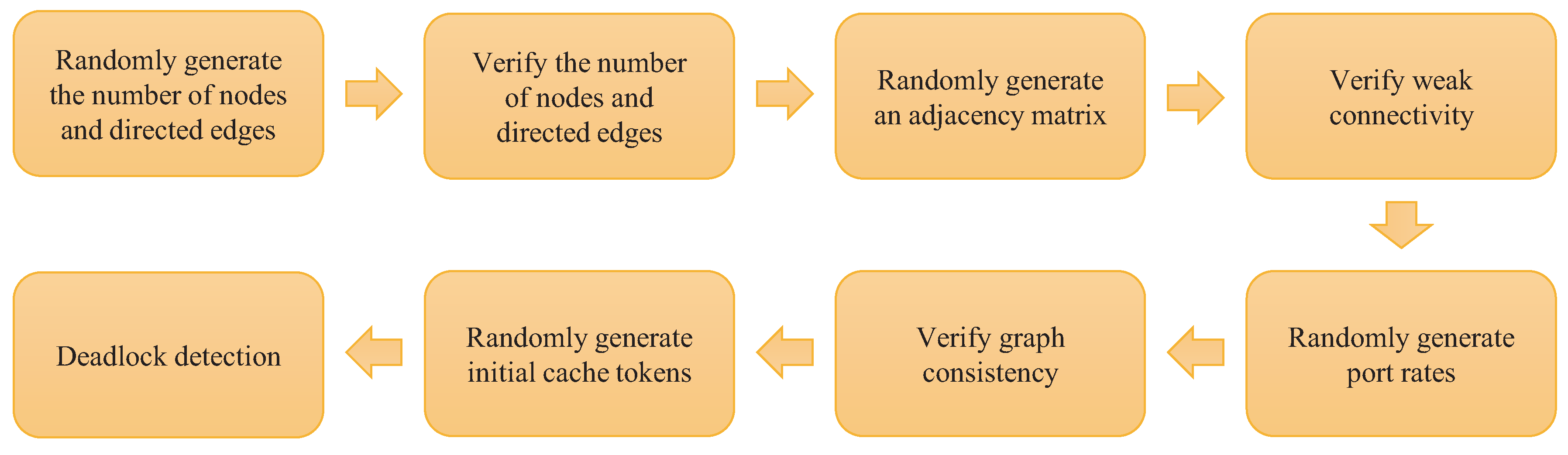
5.1. SDFG Random Generator
5.2. SDFG Data
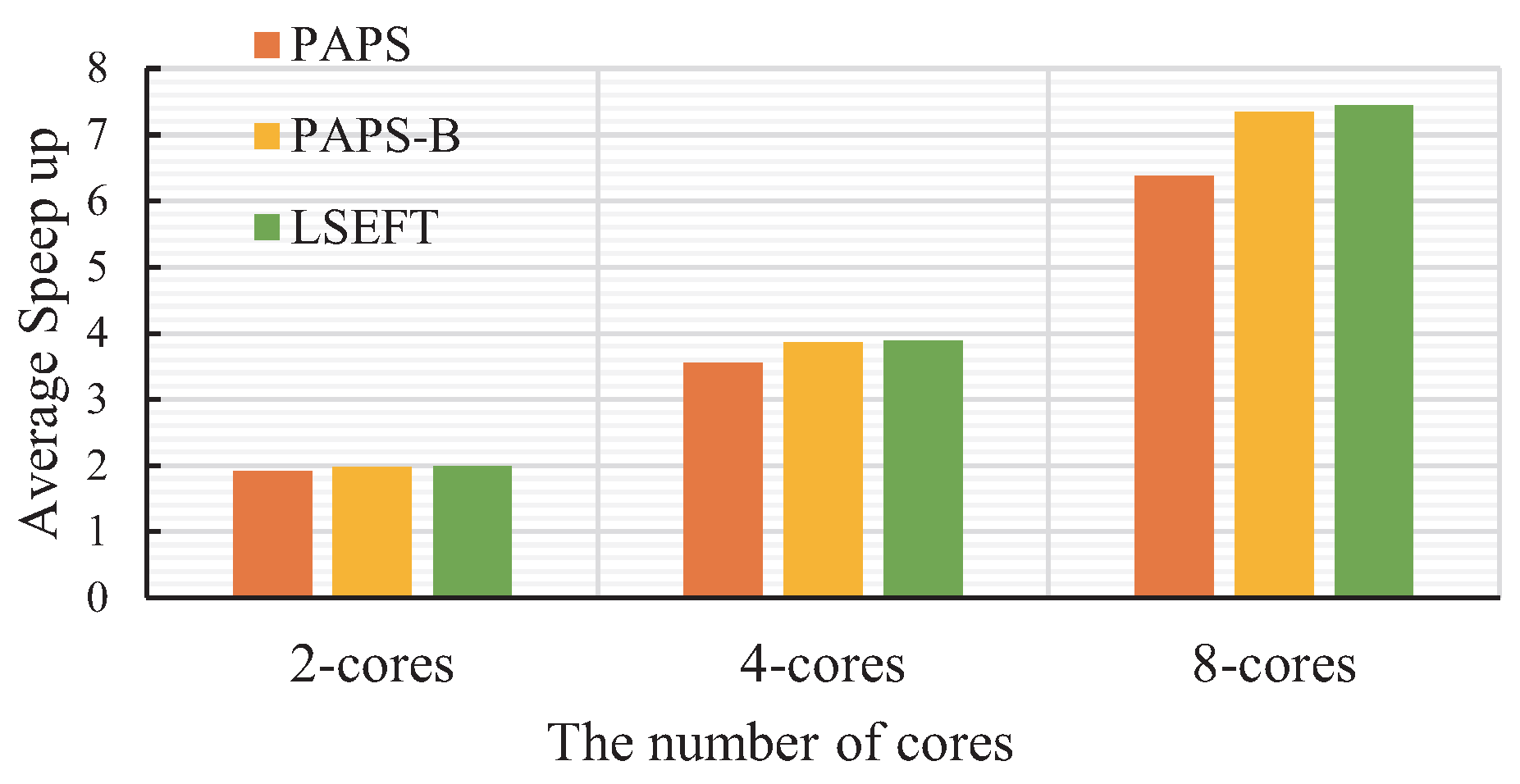
5.3. Speed Up
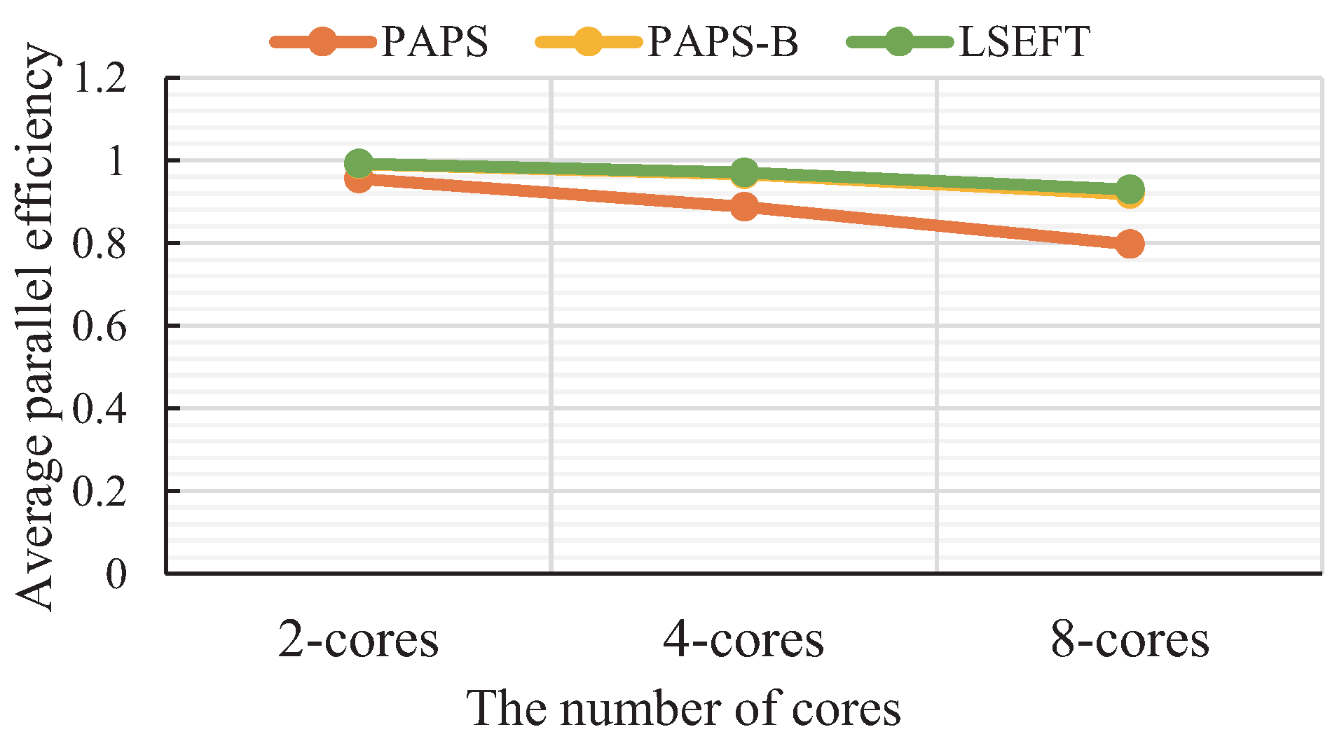
5.4. Parallel Efficiency
6. Conclusions
Author Contributions
Funding
Institutional Review Board Statement
Informed Consent Statement
Data Availability Statement
Conflicts of Interest
Abbreviations
| DAG | Directed Acyclic Graphs |
| FIFO | First In First Out |
| HSDFG | Homogeneous SDFG |
| LSEFT | Level Shortest First Earliest Finish Time |
| SDAG | Super Directed Acyclic Graphs |
| SDFG | Synchronous Data Flow Graphs |
| PAPS | Periodic Admissible Parallel Schedule |
References
- Damavandpeyma, M.; Stuijk, S.; Basten, T.; Geilen, M.; Corporaal, H. Schedule-Extended Synchronous Dataflow Graphs. IEEE Trans. Comput.-Aided Des. Integr. Circuits Syst. 2013, 32, 1495–1508. [Google Scholar] [CrossRef] [Green Version]
- Lee, E.; Messerschmitt, D. Synchronous data flow. Proc. IEEE 1987, 75, 1235–1245. [Google Scholar] [CrossRef]
- Lee, E.A.; Messerschmitt, D.G. Static Scheduling of Synchronous Data Flow Programs for Digital Signal Processing. IEEE Trans. Comput. 1987, 100, 24–35. [Google Scholar] [CrossRef] [Green Version]
- Lin, H.; Li, M.F.; Jia, C.F.; Liu, J.N.; An, H. Degree-of-node task scheduling of fine-grained parallel programs on heterogeneous systems. J. Comput. Sci. Technol. 2019, 34, 1096–1108. [Google Scholar] [CrossRef]
- Cole, R.; Zajicek, O. The APRAM: Incorporating Asynchrony into the PRAM Model. In Proceedings of the First Annual ACM Symposium on Parallel Algorithms and Architectures, SPAA’89. Santa Fe, NM, USA, 18–21 June 1989; Association for Computing Machinery: New York, NY, USA, 1989; pp. 169–178. [Google Scholar] [CrossRef]
- Suettlerlein, J.; Zuckerman, S.; Gao, G.R. An implementation of the codelet model. In Proceedings of the European Conference on Parallel Processing, Aachen, Germany, 26–30 August 2013; Springer: Berlin/Heidelberg, Germany, 2013; pp. 633–644. [Google Scholar] [CrossRef] [Green Version]
- Hu, T.C. Parallel sequencing and assembly line problems. Oper. Res. 1961, 9, 841–848. [Google Scholar] [CrossRef]
- Thies, W.; Karczmarek, M.; Amarasinghe, S. StreamIt: A Language for Streaming Applications. In Compiler Construction; Horspool, R.N., Ed.; Springer: Berlin/Heidelberg, Germany, 2002; pp. 179–196. [Google Scholar]
- Zhang, W.; Wei, H.; Yu, J. COStream: A language for dataflow application and compiler. Chin. J. Comput. 2013, 36, 1993–2006. [Google Scholar] [CrossRef]
- Veen, A.H. Dataflow Machine Architecture. ACM Comput. Surv. 1986, 18, 365–396. [Google Scholar] [CrossRef]
- Kung, S.Y.; Arun.; Gal-Ezer.; Rao, B. Wavefront Array Processor: Language, Architecture, and Applications. IEEE Trans. Comput. 1982, 100, 1054–1066. [Google Scholar] [CrossRef]
- JéJé, J. An Introduction to Parallel Algorithms; Addison-Wesley: Reading, MA, USA, 1992; Volume 10, p. 133889. [Google Scholar]
- Dorostkar, F.; Mirzakuchaki, S. List Scheduling for Heterogeneous Computing Systems Introducing a Performance-Effective Definition for Critical Path. In Proceedings of the 2019 9th International Conference on Computer and Knowledge Engineering (ICCKE), Mashhad, Iran, 24–25 October 2019; pp. 356–362. [Google Scholar] [CrossRef]
- Wu, Q.; Zhou, M.; Zhu, Q.; Xia, Y.; Wen, J. MOELS: Multiobjective Evolutionary List Scheduling for Cloud Workflows. IEEE Trans. Autom. Sci. Eng. 2020, 17, 166–176. [Google Scholar] [CrossRef]
- Djigal, H.; Feng, J.; Lu, J. Performance Evaluation of Security-Aware List Scheduling Algorithms in IaaS Cloud. In Proceedings of the 2020 20th IEEE/ACM International Symposium on Cluster, Cloud and Internet Computing (CCGRID), Melbourne, Australia, 11–14 May 2020; pp. 330–339. [Google Scholar] [CrossRef]
- Bo, Y.; Benfa, Z.; Feng, L.; Xiaoyu, Z.; Xinjuan, L.; Fang, W.; Zhitao, Z. List scheduling algorithm of improved priority with considering load balance. In Proceedings of the 2021 IEEE International Conference on Data Science and Computer Application (ICDSCA), Haikou, China, 29–31 October 2021; pp. 324–327. [Google Scholar] [CrossRef]
- Suzuki, M.; Ito, M.; Hashidate, R.; Takahashi, K.; Yada, H.; Takaya, S. Fundamental Study on Scheduling of Inspection Process for Fast Reactor Plants. In Proceedings of the 2021 2020 9th International Congress on Advanced Applied Informatics (IIAI-AAI), Tokyo, Japan, 1–15 September 2020; pp. 797–801. [Google Scholar] [CrossRef]
- Miao, C. Parallel-Batch Scheduling with Deterioration and Group Technology. IEEE Access 2019, 7, 119082–119086. [Google Scholar] [CrossRef]
- Hu, Z.; Li, D.; Zhang, Y.; Guo, D.; Li, Z. Branch Scheduling: DAG-Aware Scheduling for Speeding up Data-Parallel Jobs. In Proceedings of the 2019 IEEE/ACM 27th International Symposium on Quality of Service (IWQoS), Phoenix, AZ, USA, 24–25 June 2019; pp. 1–10. [Google Scholar] [CrossRef]
- Wu, X.; Yuan, Q.; Wang, L. Multiobjective Differential Evolution Algorithm for Solving Robotic Cell Scheduling Problem with Batch-Processing Machines. IEEE Trans. Autom. Sci. Eng. 2021, 18, 757–775. [Google Scholar] [CrossRef]
- Moi, S.H.; Yong, P.Y.; Weng, F.C. Genetic Algorithm Based Heuristic for Constrained Industry Factory Workforce Scheduling. In Proceedings of the 2021 7th International Conference on Control, Automation and Robotics (ICCAR), Singapore, 23–26 April 2021; pp. 345–348. [Google Scholar] [CrossRef]
- Yang, S.; Xu, Z. Intelligent Scheduling for Permutation Flow Shop with Dynamic Job Arrival via Deep Reinforcement Learning. In Proceedings of the 2021 IEEE 5th Advanced Information Technology, Electronic and Automation Control Conference (IAEAC), Chongqing, China, 12–14 March 2021; Volume 5, pp. 2672–2677. [Google Scholar] [CrossRef]
- Jeong, D.; Kim, J.; Oldja, M.L.; Ha, S. Parallel Scheduling of Multiple SDF Graphs Onto Heterogeneous Processors. IEEE Access 2021, 9, 20493–20507. [Google Scholar] [CrossRef]
- Bonfietti, A.; Benini, L.; Lombardi, M.; Milano, M. An efficient and complete approach for throughput-maximal SDF allocation and scheduling on multi-core platforms. In Proceedings of the 2010 Design, Automation Test in Europe Conference Exhibition (DATE 2010), Dresden, Germany, 8–12 March 2010; pp. 897–902. [Google Scholar] [CrossRef]
- Ali, H.I.; Stuijk, S.; Akesson, B.; Pinho, L.M. Reducing the Complexity of Dataflow Graphs Using Slack-Based Merging. ACM Trans. Des. Autom. Electron. Syst. 2017, 22, 1–22. [Google Scholar] [CrossRef]
- Bambha, N.; Kianzad, V.; Khandelia, M.; Bhattacharyya, S.S. Intermediate representations for design automation of multiprocessor DSP systems. Des. Autom. Embed. Syst. 2002, 7, 307–323. [Google Scholar] [CrossRef]
- Choi, J.; Ha, S. Worst-Case Response Time Analysis of a Synchronous Dataflow Graph in a Multiprocessor System with Real-Time Tasks. ACM Trans. Des. Autom. Electron. Syst. 2017, 22, 1–26. [Google Scholar] [CrossRef]
- Jung, H.; Oh, H.; Ha, S. Multiprocessor Scheduling of a Multi-Mode Dataflow Graph Considering Mode Transition Delay. ACM Trans. Des. Autom. Electron. Syst. 2017, 22, 1–25. [Google Scholar] [CrossRef]
- Bouakaz, A.; Fradet, P.; Girault, A. Symbolic Analyses of Dataflow Graphs. ACM Trans. Des. Autom. Electron. Syst. 2017, 22, 1–25. [Google Scholar] [CrossRef]
- Stuijk, S.; Geilen, M.; Basten, T. SDF3: SDF For Free. In Proceedings of the Sixth International Conference on Application of Concurrency to System Design (ACSD’06), Turku, Finland, 28–30 June 2006; pp. 276–278. [Google Scholar] [CrossRef]
- Rajadurai, S.; Alazab, M.; Kumar, N.; Gadekallu, T.R. Latency Evaluation of SDFGs on Heterogeneous Processors Using Timed Automata. IEEE Access 2020, 8, 140171–140180. [Google Scholar] [CrossRef]


| Notation | Description |
|---|---|
| An instance in set V | |
| The size of the instance | |
| The set of input channels of the instance | |
| The set of output channels of the instance | |
| The ID of input channel of the instance | |
| The ID of output channel of the instance | |
| The token producing rate of instance of channel | |
| The token consuming rate of instance of channel | |
| The execution time of the instance | |
| e | A channel in set E |
| C | A set of all processing cores |
| c | A processing core in C |
| The performance of processing core c | |
| M | The number of processing cores |
| Parameters | SDFG |
|---|---|
| Number of SDFG | 958 |
| Number of nodes | |
| Number of edges | |
| Port rate | |
| Execution time |
| Number of Instances | M | Speed Up of PAPS | Speed Up of PAPS-B | Speed Up of LSEFT |
|---|---|---|---|---|
| 8 | 2 | 1.56 | 1.56 | 1.75 |
| 32 | 2 | 1.19 | 1.33 | 1.33 |
| 64 | 2 | 1.09 | 1.09 | 1.24 |
| 128 | 2 | 1.04 | 1.20 | 1.20 |
| 8 | 4 | 2.00 | 2.00 | 2.33 |
| 32 | 4 | 1.33 | 1.33 | 1.33 |
| 64 | 4 | 1.24 | 1.24 | 2.15 |
| 128 | 4 | 1.20 | 1.20 | 2.24 |
| 8 | 8 | 2.33 | 2.33 | 2.33 |
| 32 | 8 | 1.33 | 1.33 | 2.80 |
| 64 | 8 | 1.24 | 2.04 | 3.29 |
| 128 | 8 | 2.02 | 2.02 | 3.61 |
Publisher’s Note: MDPI stays neutral with regard to jurisdictional claims in published maps and institutional affiliations. |
© 2022 by the authors. Licensee MDPI, Basel, Switzerland. This article is an open access article distributed under the terms and conditions of the Creative Commons Attribution (CC BY) license (https://creativecommons.org/licenses/by/4.0/).
Share and Cite
Wang, L.; Wang, C.; Wang, H. Improved Scheduling Algorithm for Synchronous Data Flow Graphs on a Homogeneous Multi-Core Systems. Algorithms 2022, 15, 56. https://doi.org/10.3390/a15020056
Wang L, Wang C, Wang H. Improved Scheduling Algorithm for Synchronous Data Flow Graphs on a Homogeneous Multi-Core Systems. Algorithms. 2022; 15(2):56. https://doi.org/10.3390/a15020056
Chicago/Turabian StyleWang, Lei, Chenguang Wang, and Huabing Wang. 2022. "Improved Scheduling Algorithm for Synchronous Data Flow Graphs on a Homogeneous Multi-Core Systems" Algorithms 15, no. 2: 56. https://doi.org/10.3390/a15020056
APA StyleWang, L., Wang, C., & Wang, H. (2022). Improved Scheduling Algorithm for Synchronous Data Flow Graphs on a Homogeneous Multi-Core Systems. Algorithms, 15(2), 56. https://doi.org/10.3390/a15020056