Data Fitting with Rational Functions: Scaled Null Space Method with Applications of Fitting Large Scale Shocks on Economic Variables and S-Parameters

Abstract

Curve fitting discrete data (x, y) with a smooth function is a complex problem when faced with sharply oscillating data or when the data are very large in size. We propose a straightforward method, one that is often overlooked, to fit discrete data ($s$, $y_s$) with rational functions. This method serves as a solid data fitting choice that proves to be fast and highly accurate. Its novelty lies on scaling positive explanatory data to the interval [0, 1], before solving the associated linear problem $\mathrm{A}x=0$. A rescaling is performed once the fitting function is derived. Each solution in the null space of A provides a rational fitting function. Amongst them, the best is chosen based on a pointwise error check. This avoids solving an overdetermined nonhomogeneous linear system $\mathrm{A}x=b$ with a badly conditioned and scaled matrix A. With large data, the latter can lack accuracy and be computationally expensive. Furthermore, any linear combination of at least one solution in the basis of the null space produces a new fitting function, which gives the flexibility to choose the best rational function that fits the constraints of specific problems. We tested our method with many economic variables that experienced sharp oscillations owing to the effects of COVID-19-related shocks to the economy. Such data are intrinsically difficult to fit with a smooth function. Deriving such continuous model functions over a desired period is important in the analysis and prediction algorithms of such economic variables. The method can be expanded to model behaviors of interest in other applied sciences, such as electrical engineering, where the method was successfully fitted into network scattering parameter measurements with high accuracy.

1. Introduction

Fitting data with smooth functions, polynomials, rational functions, and others is an increasingly growing topic of interest in the fields of data science, machine learning, all engineering disciplines, political and social sciences, medicine and pharmaceutical sciences, economics, finance, and many others. The fitting function is considered a mathematical continuous model obtained from discrete experimental measurements. A few examples of the vital applications are data recovery in imaging, extrapolation, converting discrete frequency measurements to a continuous time-domain simulation in electrical and mechanical systems via Fourier transform, data mining, machine learning, neural networks, and statistical predictors algorithms used in stock prices predictions software.

There are various fitting methods in the literature, and they all have advantages and disadvantages. In ref. [1], a survey of many fitting methods with rational functions is presented along with performance comparative examples. Some of the fitting techniques are: Bode’s asymptotic approximation [2], the Levy method [3], iteratively reweighted least squares [4,5], the Sanathanan–Koerner method [6], the Noda method, Vector Fitting along with its improvement [7,8], the Levenberg–Marquardt method and its updates [5,9,10], and the Damped Gauss–Newton method [4].

These methods solve the problem of finding a rational curve fitting function $f$ that takes the general form from discrete measurements $\left(s,y_s\right)$, which is substituted in the above equation for $\left(z,f\left(z\right)\right)$. A linear system $\mathrm{A}x=b$ is then derived to solve for the coefficients $a_i \mathrm{and} b_i$.

Most of the mentioned rational approximation techniques are iterative and rely on a clever choice of an initial guess. The behavior and size of data control the success or failure of the methods. With sharply oscillating data, convergence fails or performs slowly. Also, accuracy of the approximation would not be achieved with a less refined initial guess [11].

Furthermore matrix $\mathrm{A}$ is badly scaled with high magnitudes of s and N, which also affects convergence and accuracy. The presented method in this work is a noniterative method, and therefore we do not incorporate an initial guess. Moreover, scaling explanatory data s to the interval [0, 1] before deriving the linear system solves the badly scaled matrix A issue, and therefore results in higher stability and accuracy compared to that of methods that did not scale measurement s. We believe that the scaling process is what set the presented method apart from others, coupled with the use of the “extraordinary SVD method” as described in the work of Martin and Porter [12] to solve a homogeneous system.

In Section 2, we present the mathematical derivation of the method. In Section 3, we apply scaled null space technique to model various economic variables that experienced sudden shocks due to COVID-19 impact on US economy during the recession that started in March 2020. We believe that since the model could fit the data for such a period of unstable trends in the economic variables, it is expected to perform better with data that does not manifest such strong oscillations. We used our method to model two stock market indices: Dow Jones Index Average (DJIA) and Standard and Poor’s 500 (S&P 500); two US treasury bonds yields: the 3-month treasury bond and 10-year treasury bond; and unemployment rate. Although the actual data go through large shocks, our model is accurate in approximating the data with low residual errors. In Section 4, we compare the results of our proposed method with the Matlab rationalfit method and the results with the unscaled version of our method. In the same section, we present a recovery example of the sine function from sampled points selected from its curve. Finally, we discuss in Section 5 limitations of the presented method, a proposed approach to overcome failure to accurately fit the data, and an example to approximate very large data of sinusoidal behavior.

2. Methodology: Null Space on Scaled Independent Variable

The goal of the method presented in this section is to fit discrete data measurements ($s$, $y_s$) with a real valued rational function $f$ where s is the explanatory variable and $y_s$ is the response variable. We consider the fitting function $f$ to be in the form

$$f\left(z\right)=\frac{a_0+a_{1}z+a_2{z}^2+\cdots a_N{z}^N}{b_0+b_{1}z+b_2{z}^2+\cdots b_N{z}^N}$$

(1)

for real value z. When the responses $y_s$ are complex numbers, as in many engineering systems, the fitting technique can be broken down into fitting separately the real and imaginary parts of $y_s$.

Before we proceed with the derivations, we normalize the explanatory variable data s in the infinity norm sense. So, all values s will be replaced with $\frac{s}{s_{max}}$, where $s_{max}$ is the maximum value among all |s|. This scaling process allow all powers of s to be contained in the interval [0, 1] for positive s. For each value s, Equation (1) becomes:

$$y_s(b_0+b_{1}s+b_2{s}^2+\cdots b_N{s}^N)-(a_0+a_{1}s+a_2{s}^2+\cdots a_N{s}^N)=0$$

which gives

$$b_0{y}_s+b_{1}s{y}_s+b_2{s}^2{y}_s+\cdots b_N{s}^N{y}_s-a_0-a_{1}s-a_2{s}^2-\cdots -a_N{s}^N=0$$

The unknowns are the coefficients in the vector $\left(b_0,b_1,b_2,\dots ,b_N,a_{0 },a_{1 },a_2\dots a_N\right)$. Once we solve for the coefficients, a fitting function is defined.

Suppose we have m data (s,$y_s$). Each pair of measurement gives an equation, and therefore we obtain a homogeneous system of m equations represented in matrix form:

$$\mathrm{A}x=0$$

(2)

where $x=\left(b_0,b_1,b_2,\dots ,b_N,a_{0 },a_{1 },a_2\dots a_N\right)$’ and A is the coefficient matrix with size m by 2N + 2. Each couple (s,$y_s$) defines a row in the matrix A,

$$(y_s y_{s}s y_s{s}^2\dots y_s{s}^N -1 -s -s^2\dots -s^{N })$$

The benefit of scaling by 1/$s_{max}$, where all powers of s are contained in the interval [0, 1], is evident. This avoids a badly scaled coefficient matrix A, especially for higher s and N.

The set of vector solutions $x=\left(x_1,x_2,\dots ,x_r\right)$ form a basis of the null space of A, null(A). With the proper choice of the degree N, each solution vector $x_i , 1\le i\le r$ gives a rational fitting function $f_i$. The best rational function $f$ is picked by calculating the minimum of the errors $\left||f_i-y_s\right|{|}_{\infty }$, where $f_i$ is the evaluation vector with inputs $s$ using Equation (1), and $y_s$ is the vector of the data responses $y_s$.

In other words, the index n, that gives the best fitting function $f_n$ is defined by

$$||f_n-y_s|{|}_{\infty }=\underset{1\le i\le r}{\min }||f_i-y_s|{|}_{\infty }$$

The vector $f_n$ contains the coefficients of the model function $f_n$.

This process is our preferred error minimization method between the response observations $y_s$ and the function coefficients in $f_i$. The users can choose an alternative minimization norm such as the 2-norm for instance. Next, we horizontally stretch the fitting function by a factor of $s_{max}$ to be defined on the original interval containing the raw unscaled variable $s$, i.e., the fitting function is giving by

$$f\left(z\right)=f_n\left(s_{max}z\right)$$

(3)

To solve Equation (2) we used MATLAB built-in function null(A), which is based on the singular value decomposition (SVD) of matrix A. When A is very large the economy-sized MATLAB svd(A,”econ”) can be used. This method also extends for negative values of $s$, in which case scaled values $\frac{s}{s_{max}}$ will be contained in the interval [−1, 1], and so are all powers of s. The existence of infinitely many solutions is guaranteed when the system $\left(2\right)$ is underdetermined $\left(m<2N+2\right)$. In fact, the dimension of the null space is always at most $\left(2\mathrm{N}+2-\mathrm{m}\right)$. When the system is overdetermined or A is a square matrix $\left(m\ge 2N+2\right)$, we need enough linearly dependent equations for the solutions to exist, precisely at most $2N+1$ linearly independent equations. If the latter condition is not satisfied, we should increase the degree $N$ until either we have an underdetermined system or $2N+1$ linearly independent equations if the system remains overdetermined. In general, the degree of the polynomials $N$ is higher with more fluctuating data. It is also higher with a larger amount of data.

3. Results and Discussion

Modeling discrete data responses with a continuous smooth function can be used as a future predictor, when fit, to anticipate similar behavior in economics, finance, public health, sociology, etc. [13]. It can also be used as a base to derive momentum oscillators and be implemented in learning algorithms crucial to profitability of technical stock trading, for instance [14,15,16,17].

In this section, we apply our method on examples from the shock that hits the economy early in the onset of COVID-19 pandemic. During the early onset of COVID-19 in March and April of 2020, financial markets were very volatile given the uncertainty about the future. Financial literature showed that uncertainty about the near-term or long-term future leads to large spreads in bond markets and high volatility in the financial markets. In [18], the authors even show that stock market uncertainty has important cross-market pricing influences and that stock-bond diversification benefits increase with stock market uncertainty. In addition, Federal Reserve intervened to calm the markets by lowering the key interest rate and creating various special lending programs to provide liquidity for the financial system and for local and state governments. All these unique developments created a chaotic scenario for many of the economic variables to experience huge swings. Indeed, the effects of COVID-19 developments and policy responses on the US stock market and bond markets are without historical precedent [19]. We choose this period given its large uncertainty about the future and its erratic oscillations in all economic and financial variables during this period. We included examples from Dow Jones Index Average (DJIA), Standard and Poor’s 500 (S&P 500), two treasury rates such as 3-month treasury bond rate and 10-year treasury bond rate, and unemployment rate. We collected data from publicly available sources such as Federal Reserve Economic Data, which is published by Federal Reserve Bank of St. Louis [20].

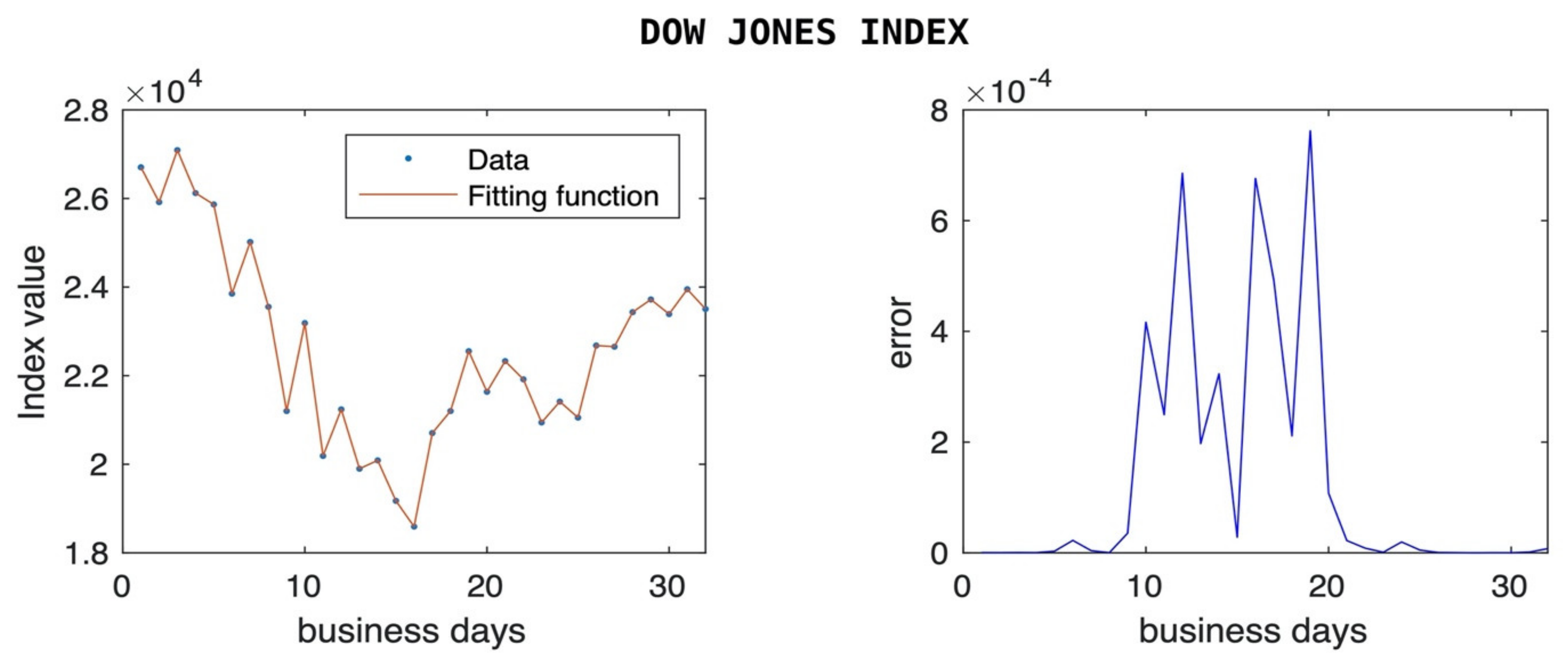
For each data sample, a graph of the fitting function versus raw observations is presented along with a pointwise error plot. The method was capable of fitting data with frequent zigzagging, especially in the DJIA and S&P 500 index examples.

In the following examples the error figures represent the absolute value of the difference between the response observations $y_s$ and the corresponding values of the fitting function, $error=\left|f\left(s\right)-y_s\right|$. As in Equation (1) in the previous section, we denote N, the order of the polynomials in the numerator, and the denominator of the fitting function f.

In Figure 1 and Figure 2, we show how the stock market indices reacted to the news of the COVID-19 pandemic. DJIA is one of the oldest and most commonly used equity indices in the market, representing a price weighted index of 30 large companies. The figures show that DJIA lost more than 32% of its value within a few days in mid-March, and it was able to recover most of it back within a couple of weeks. The figures include only business days since there are no data for stock market and bond market during the weekends.

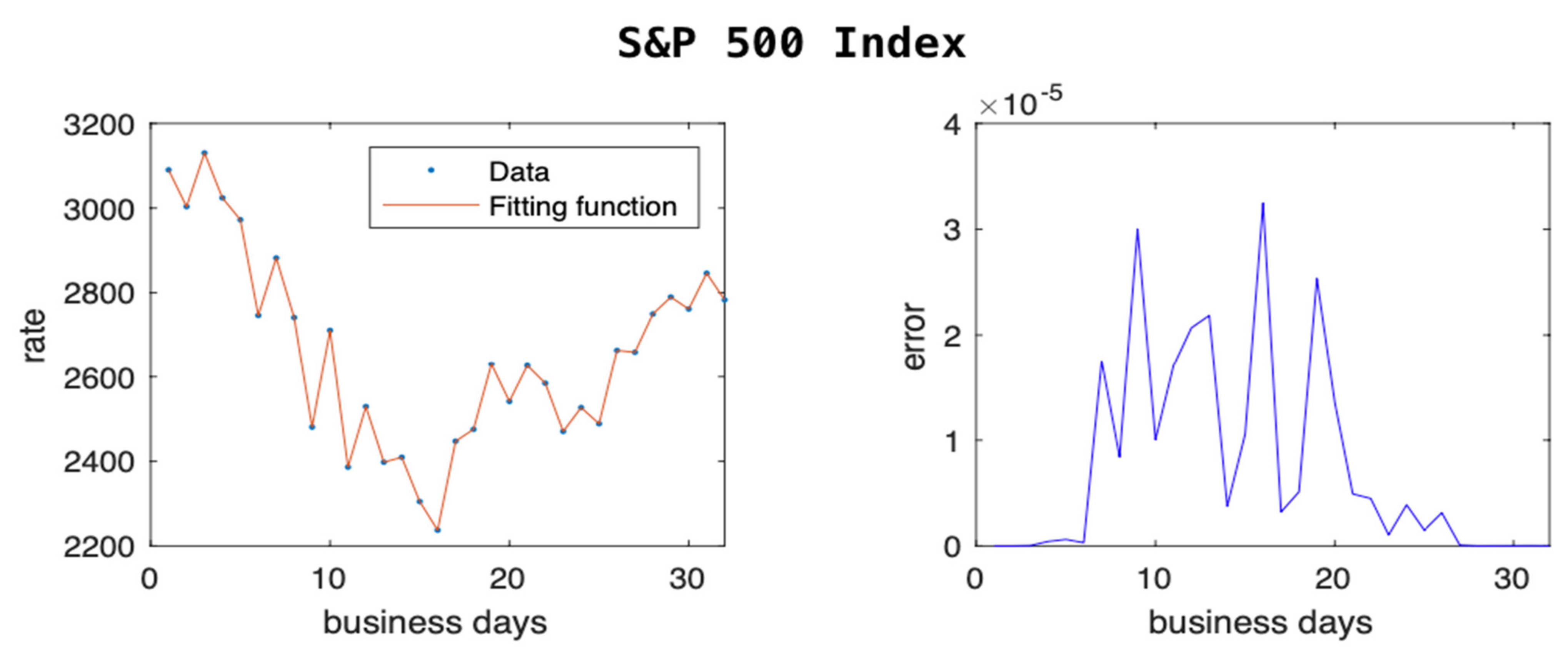
In Figure 2, we show the trend of S&P 500, which tracks the performance of 500 large companies listed on the stock exchanges in the US. Even here we can see a drop of about 28% in the value of the index and a quick recovery of most of that loss within a few weeks. Our model is able to predict with low error these zigzagging trends.

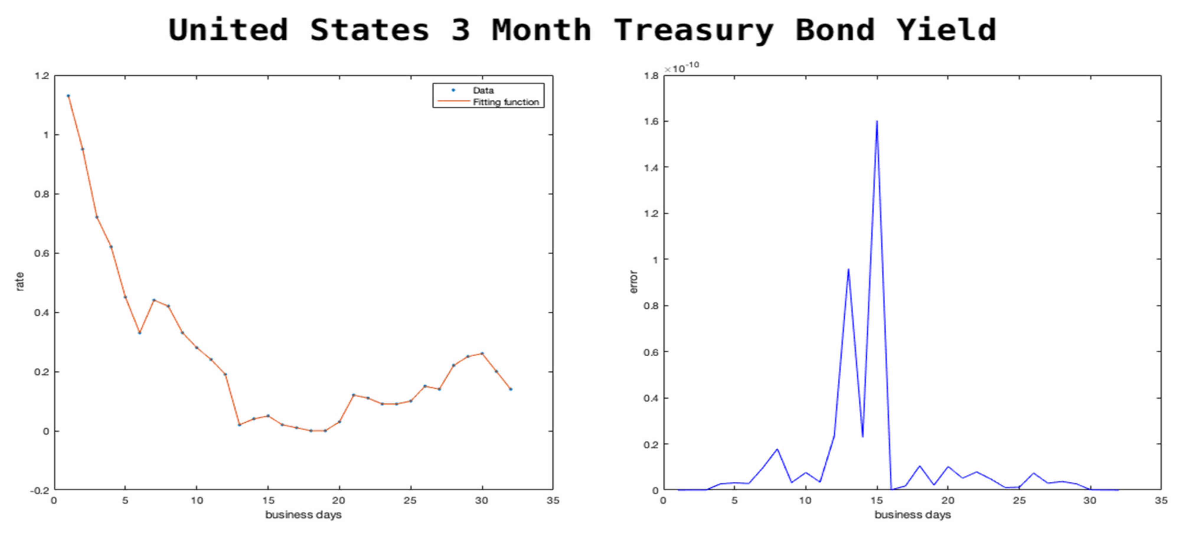
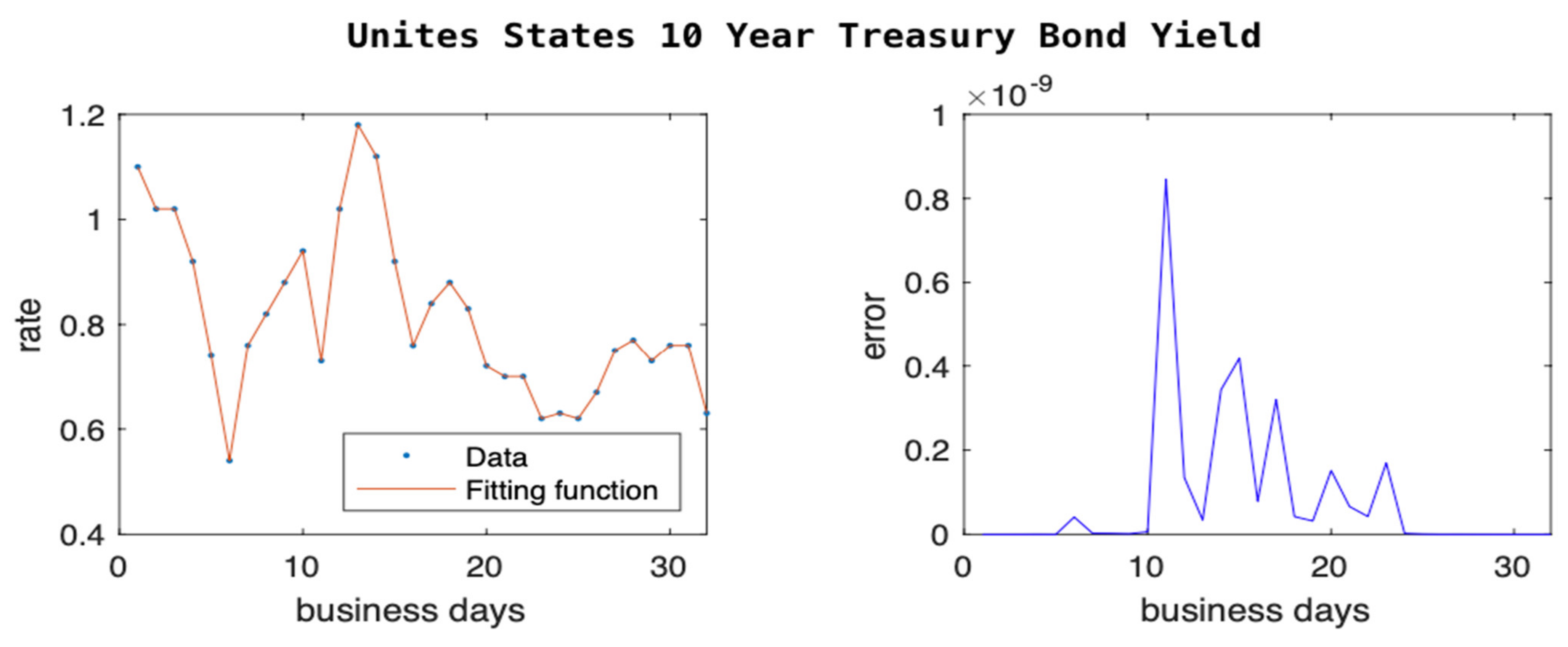
In Figure 3 and Figure 4, we show the trend of the two treasury bond rates. We chose to focus on these two bonds rates because one is very short-term (3 months) and one is long-term (10 years). The short-term one is the cost of borrowing on money markets for a short period, while the long-term one is a proxy for the cost of investment. Many companies choose to borrow for investment and borrow based on the cost of borrowing for a long-term project, which is usually at a higher premium compared to that of the treasury bond.

In February 2020, the interest rates of the two bonds were similar, and many financial economists were predicting a potential economic crisis due to expectations of lower long-term interest rates. After the announcement of the pandemic by the World Health Organization on 11 March 2020, Federal Reserve slashed its own key interest rate and started purchasing treasury bonds. This movement led to drastic changes in the interest rates as seen in Figure 3 and Figure 4. However the effect was much larger on the short-term interest rates as the markets expected the shock to be short-lived. Our models predict the trend within low errors as seen on the right side of the figures.

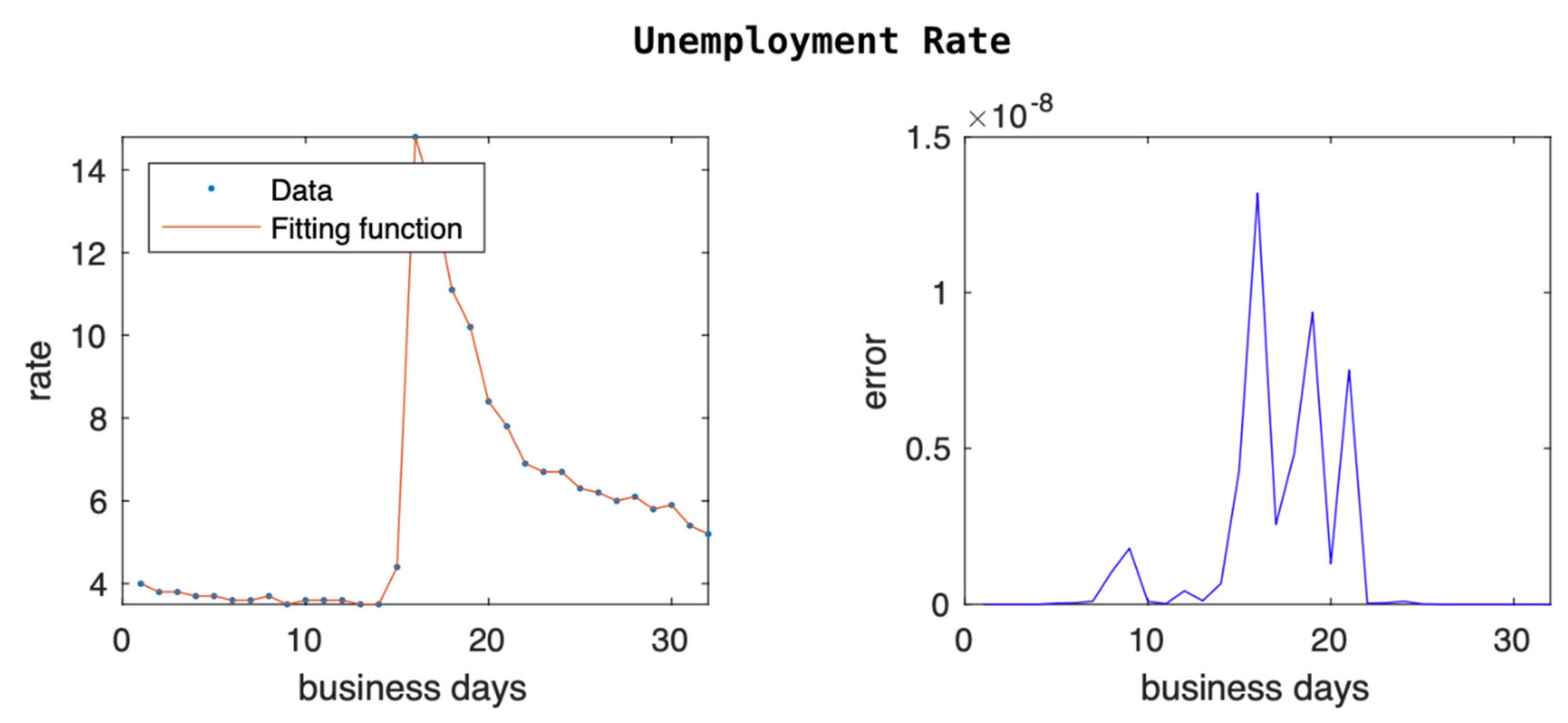
Our last example with economic data is the unemployment rate, and we can see the data and the error fitting of our model in Figure 5. Given that the unemployment rate data are monthly, we expand our sample from January 2019 to August 2021. The unemployment rate was decreasing to historical lows until COVID-19 hit. Due to forced shutdowns the number of layoffs increased dramatically, going from 3.5% to 14.8%. As the economy started reopening slowly, we saw the unemployment rate coming down slowly. Our model was able to cope with the sharp spike of the unemployment rate and approximated the responses within very small errors, as shown in Figure 5.

We tested our model with extreme cases where the actual historical data have experienced large fluctuations. We showed that our model is able to predict with an extremely low number of errors (as low as 0) that the 10-year treasury bond rate, in which there were instances of large swings in data, showed approximately 100% fluctuation within a few days (see Figure 4). If the model can perform at this level, in extreme cases like the ones shown above, one can expect even higher accuracy (lower errors) in the case of relatively lower fluctuations as presented in the next sections.

4. A Comparative Performance of the Model

In this section, we present two examples to perform a comparison between a Matlab bult-in function rationalfit and our method.

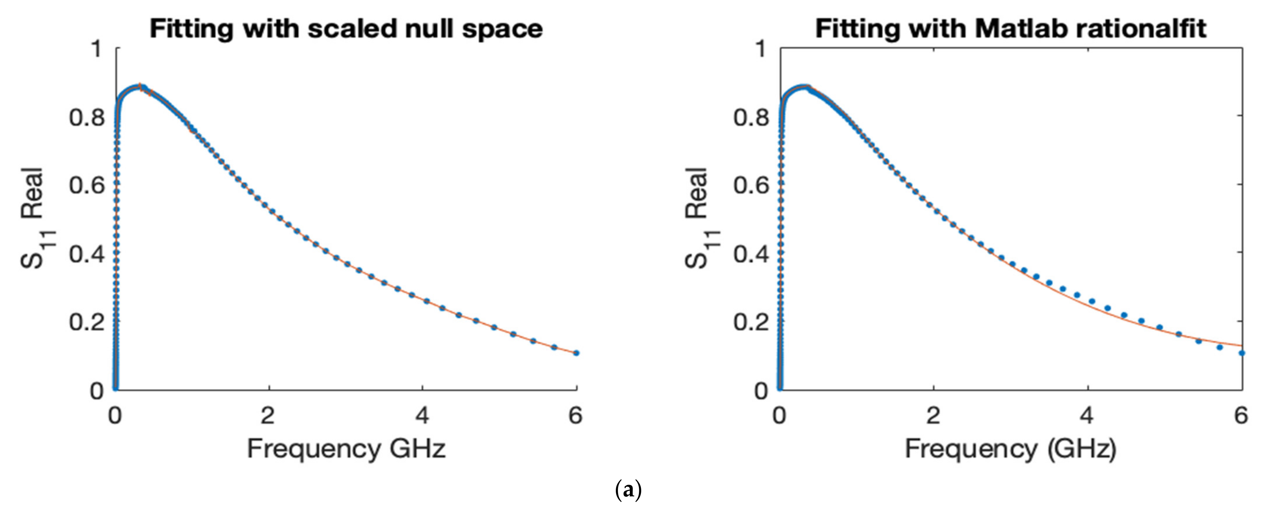
4.1. Comparison on Network Scattering Parameters Data $S_{11}$

The first comparative example is concerned with fitting network scattering parameter data. Network scattering parameters are powerful tools for the analysis and design of high-frequency and microwave networks, and they can be tested by users in a guided example with Matlab Radio Frequency toolbox [21,22]. As stated in Matlab R2021b release documentation, rationalfit approximates data using stable rational function object and is based on vector fitting method [1], along with its improvement [23]. The original paper [1] gained popularity in the electrical engineering community, with high number of paper citations and patent. The data in this example are the same used by the author to illustrate its robust performance in fitting S-parameters. We compared the model functions obtained by both schemes to fit the real and imaginary parts of the responses $S_{11}$ along with their corresponding errors, Figure 6, Figure 7, Figure 8 and Figure 9.

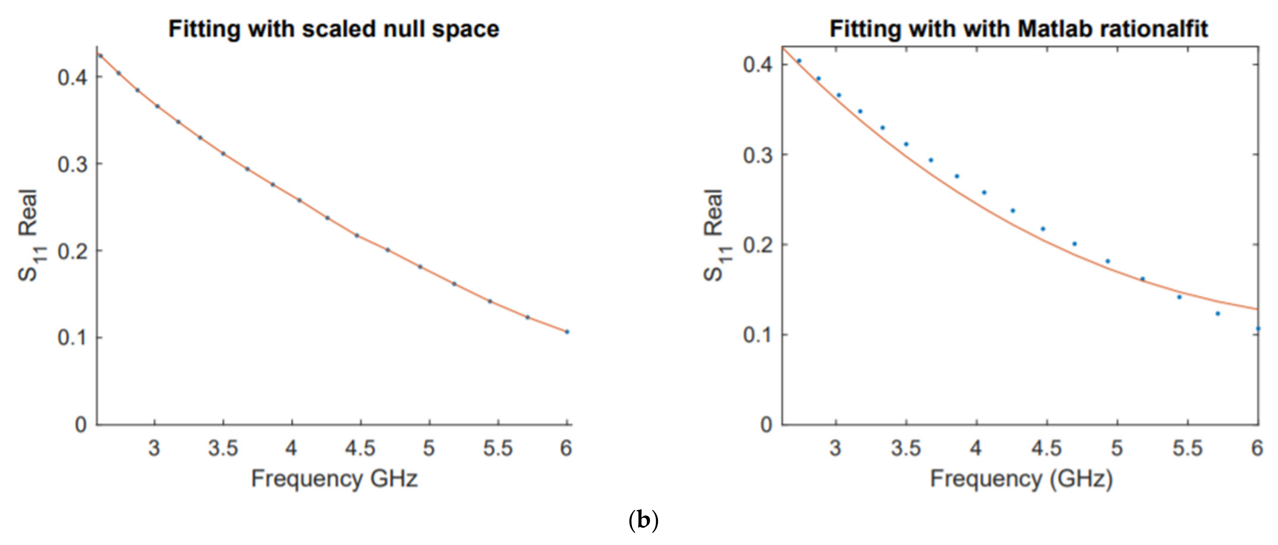
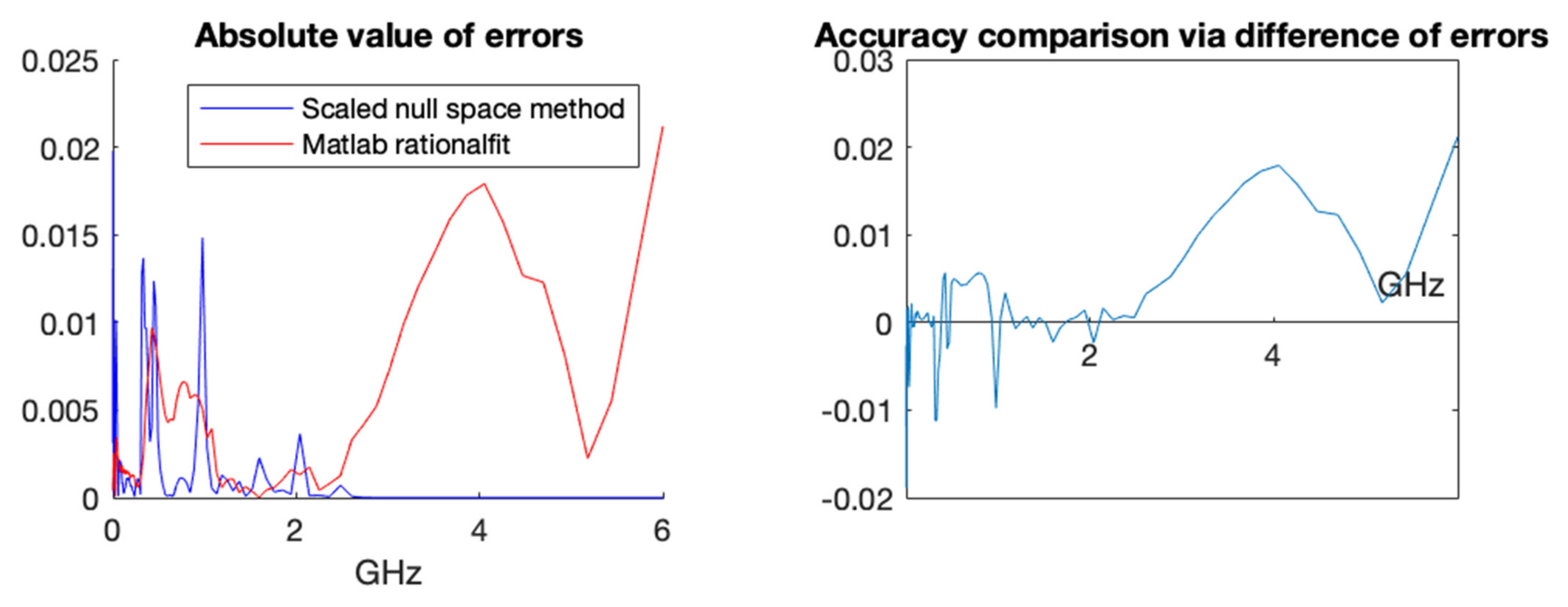
A more in-depth comparison is presented below in Figure 7 with a pointwise error plot of each method and a difference plot between the errors (error with rationalfit minus error with scaled null space).

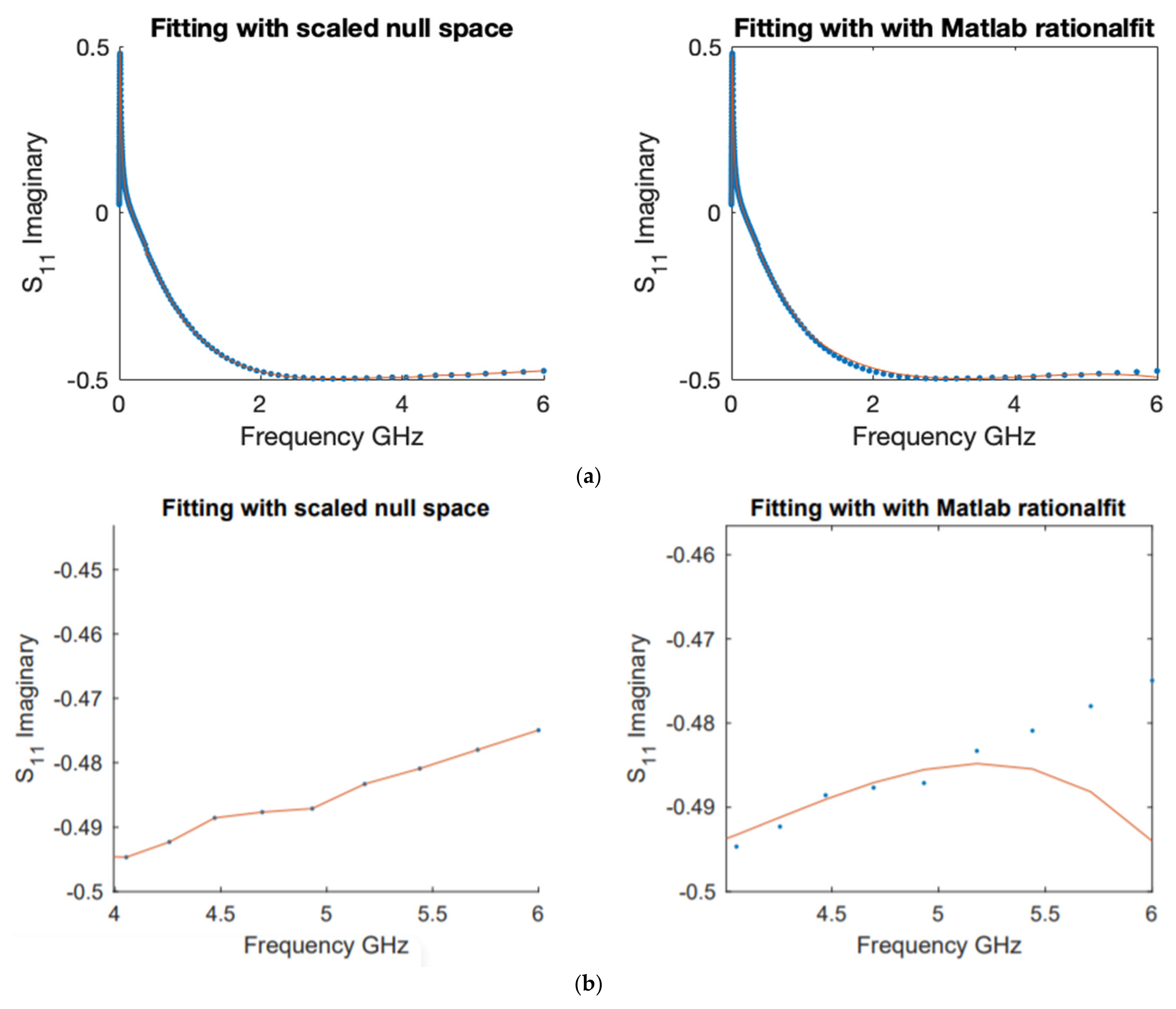
Next, we show a similar profile when we fit the imaginary part of the responses in terms of frequencies. These comparisons are reported in Figure 8 and Figure 9. First, we report the fitting of both methods with scaled null space and with Matlab rationfit method in Figure 8.

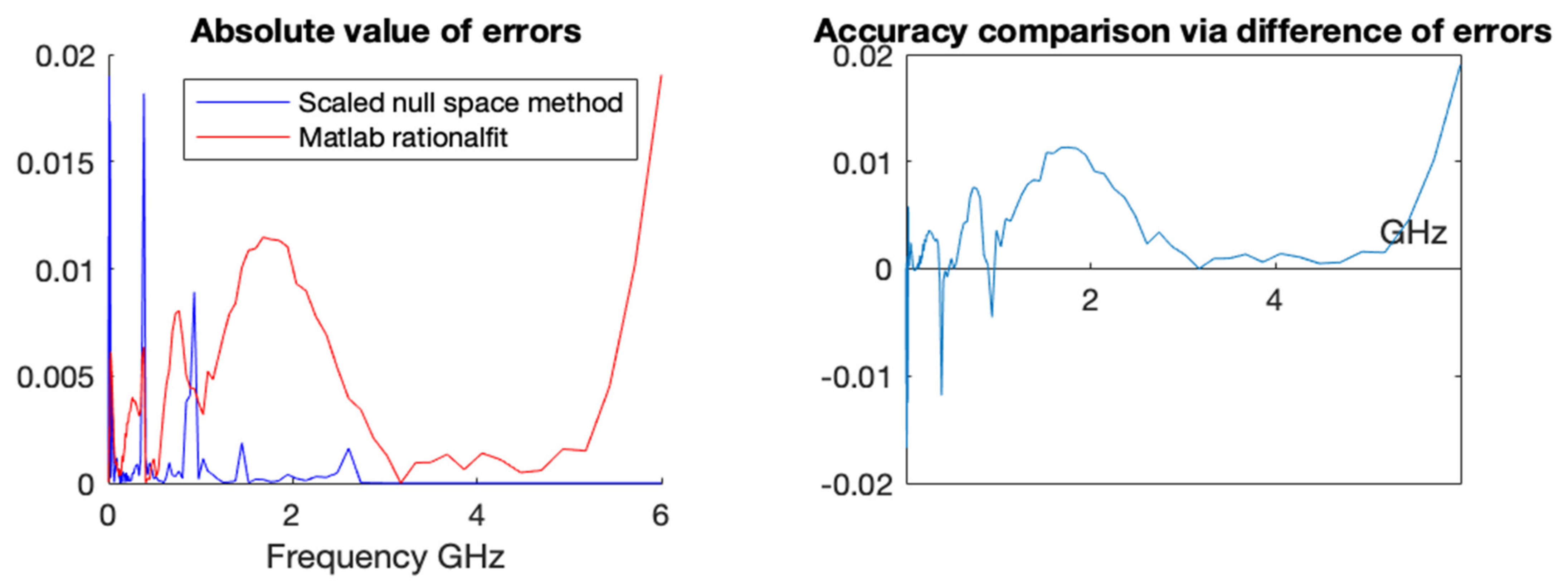
In Figure 9, we show a pointwise comparison that illustrates the error plot and the difference between the magnitude of the errors (error with rationalfit minus error with scaled null space).

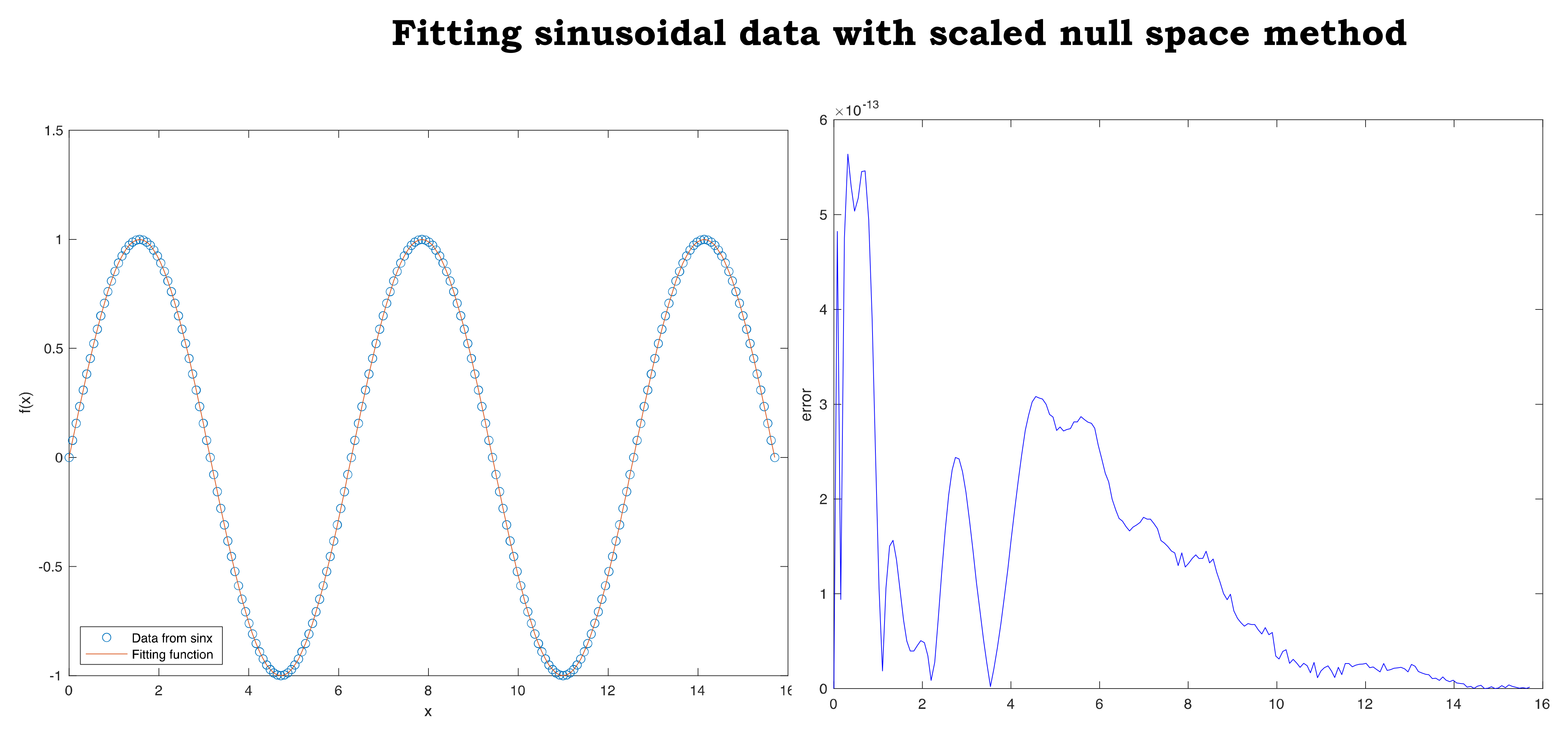
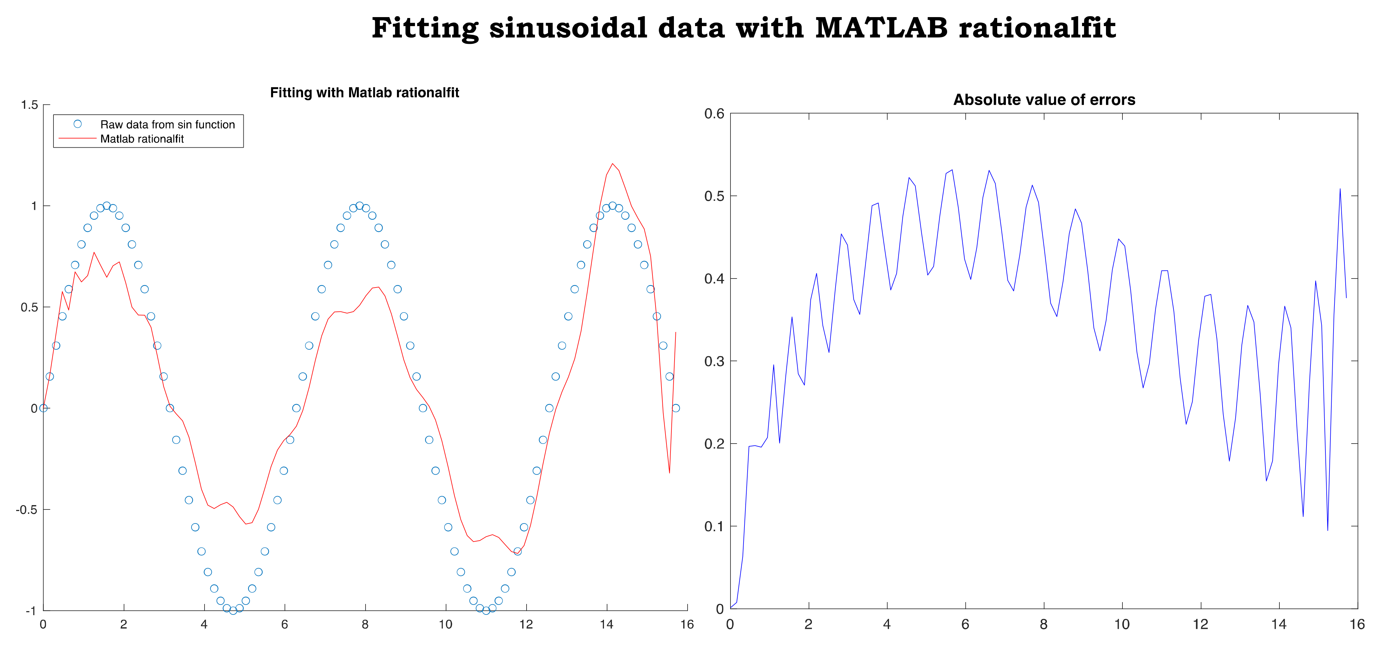
4.2. Comparison on Sinusoidal Behaving Data

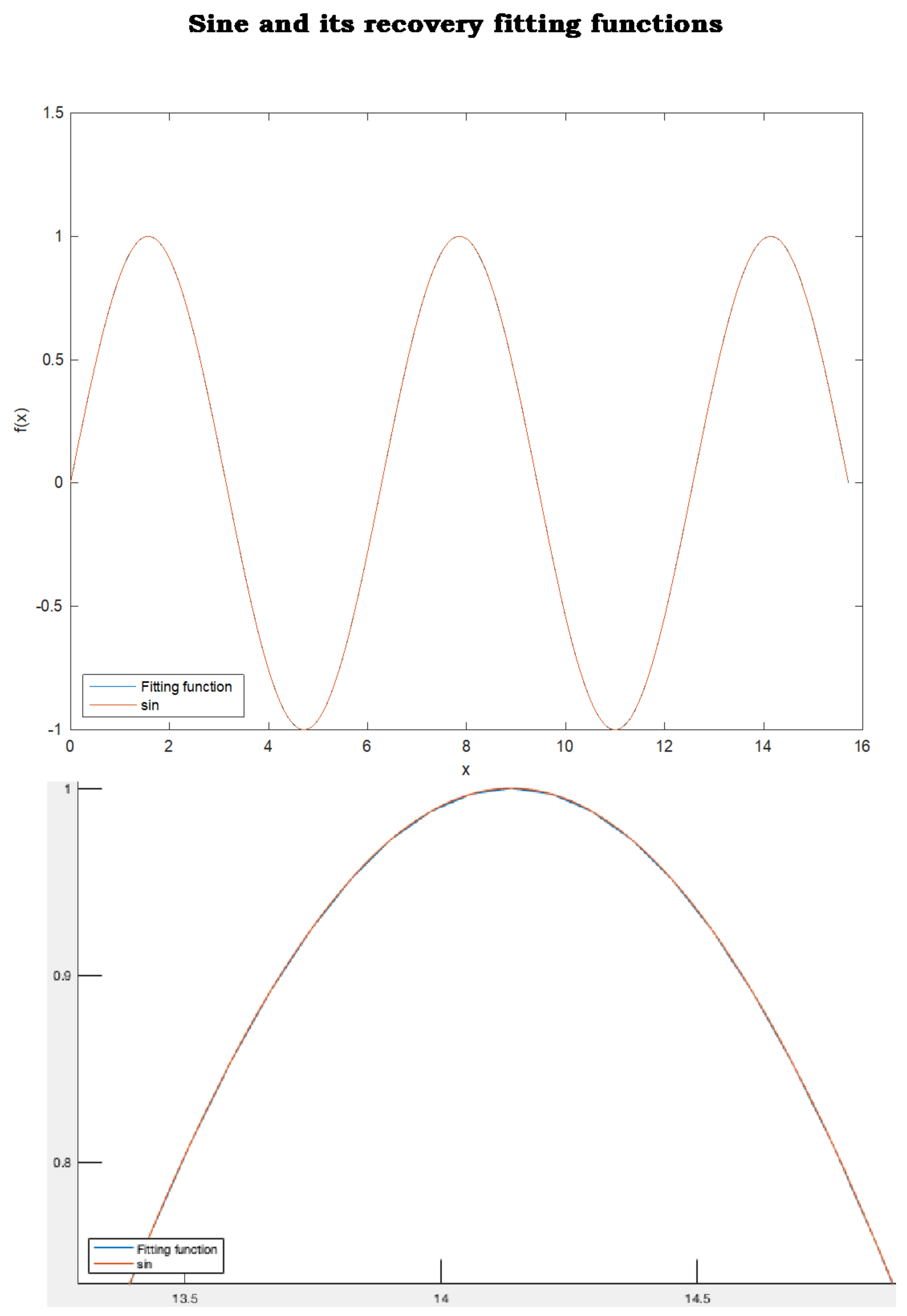
The second comparative example begins with fitting a sample (x, y) of 201 points uniformly spaced, extracted from the sine function over the interval $\left[0, 5\pi \right].$ This example shows high accuracy of fitting sinusoidal behaving data that arise in many applications, Figure 10. In addition, we show the capability of the fitting function to recover, with high precision, data not included in the sample, Figure 11. In fact, every real value in $\left[0, 5\pi \right]$ not listed in the 201 sample points is recovered with high accuracy by the fitting function provided by scaled null space method. The sine function and the rational fitting function are almost overlapping everywhere in $\left[0, 5\pi \right]$. In other words, if the sine function was unknown and was only represented by a sample of 201 data uniformly distributed over $\left[0, 5\pi \right]$, then scaled null space method would have recovered the sine function with high accuracy over the entire interval $\left[0, 5\pi \right]$. MATLAB rationalfit did not return an adequate fitting of the same data, Figure 12. Furthermore, at the end of this subsection, we fit the same data $S_{11}$ with the unscaled version of our method to highlight the importance of the scaling procedure, Figure 13.

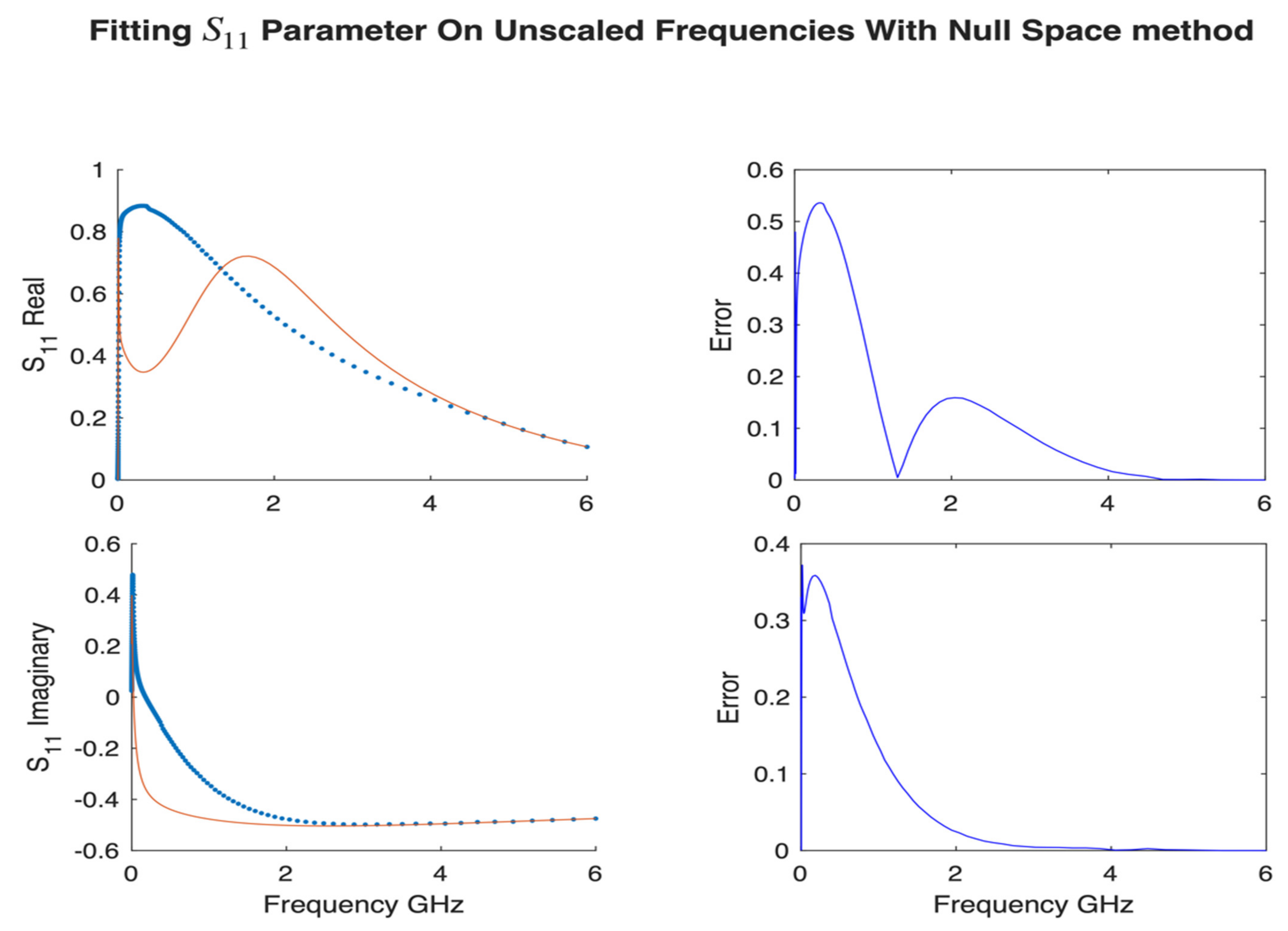
Lastly, we show the performance of our method without scaling the frequencies $s$ by ${\frac{1}{s}}_{max}$ in Figure 13. As we discussed in Section 2, the coefficient matrix A is badly scaled due to the high powers $s^i$ for large $s$ and $i$. We used the same s-parameters data presented above for accuracy comparison with scaled null space method.

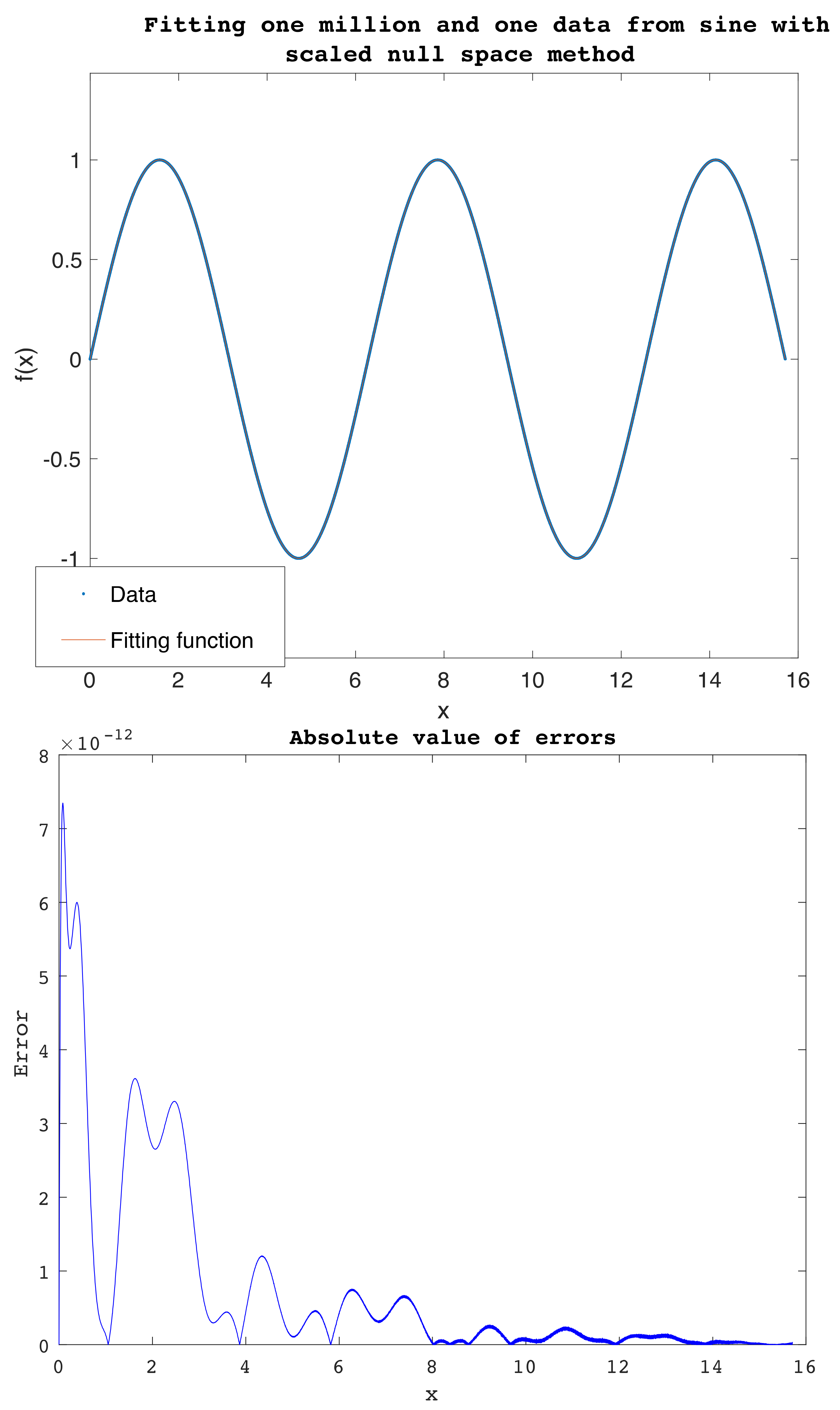
5. Fitting Large Data and Limitations

There are challenges that face fitting experimental data (x, y) with smooth functions. These challenges impede many successful curve fitting methods from being universal, meaning the capability of performing smoothing of any data (x, y) regardless of their complexity. One of the challenges is the behavior of the data, especially data manifesting frequent sharp oscillations, as in the examples of stock prices. The latter limitation is intrinsic as the data have many corners and the fitting function is smooth. Another limitation is the large size of the data leading to large scale linear systems with very large coefficient matrices that could be ill-conditioned or badly scaled. Furthermore, large data exacerbate convergence failure and speed issues in iterative fitting methods such as Levenberg–Marquardt. Fitting with a smooth function data with both limitations present simultaneously is a very complicated problem. Our method fails to provide adequate accuracy when both conditions meet in certain data, as any fitting method would do. The highest number our method was successful to fit is one-million-and-one (${10}^6+1$) pairs (x, y) extracted from the sine function over $\left[0, 5\pi \right]$ (Figure 14), with pointwise errors less than 7.4 × ${10}^{-12}$ over all the one-million-and-one points. These small residuals show a clear advantage of our method when fitting very large data that behave smoothly enough. Matlab rationalfit failed to fit 201 data extracted from the same function as discussed in the previous example.

As a proposed remedy, when the method fails to return a desired precision, the user should resort to partitioning the data over subintervals and fit them over each one. The overall fitting function is a piecewise continuous function with negligible jump discontinuities. In other words, let us consider the partition of the data over $x$ into n subintervals

$$I_{i=}\left[x_i, x_{i+1}\right), 1\le i\le n-1, I_{n=}\left[x_n, x_{n+1}\right].$$

Let $f_i$ be a good rational fit over $I_i$ obtained either by our method or any other method. The overall fitting function $f$ writes:

$$f={\displaystyle \sum }_{i=1}^n{f}_i {\chi }_{I_i}$$

where ${\chi }_{I_i}$ is the characteristic function ${\chi }_{I_i}\left(x\right)=\left\{\begin{array}{c}1, if x\in I_i\\ 0,if x \notin I_i \end{array}\right.$.

The jump discontinuities ${\epsilon }_i=\left|f_i\left(x_{i+1}\right)-f_i\left(x_i\right)\right|, 1\le i\le n$ are small when the functions $f_i$ perform well the curve fitting over $I_i.$ In many practical applications, such derivation is sufficient as in numerical integration of a function given as discrete pairs (x, y) for instance.

6. Conclusions and Future Expansion

The presented method in this work has a few advantages. First, it fits with rational functions, which are proven to be reliable at coping with many data behaviors. Second, the mathematics of finding the best fitting rational function is straight forward and is based primarily on solving a homogeneous linear system or finding the null space of a matrix, which can be performed efficiently in numerous ways [11]. Lastly, generating a null space base is efficiently computed via the “Extraordinary SVD” method as described in the work of Martin and Porter [12]. This will take away much of the burden in solving an overly determined, nonhomogeneous system Ax = b with optimization techniques; a task that is more challenging when the matrix A is badly scaled and conditioned, which is the case when trying to solve for the coefficients in $f\left(s\right)$ via a nonhomogeneous system [1]. The latter limitation was the drive behind straying away from a direct approach when fitting with rational functions [1,2].

In this paper, we proposed a robust method to fit data ($s$, $y_s$) with rational functions. We transformed the problem to a null space problem on scaled explanatory data. The presented method has a few advantages: First, we fit data with rational functions that are flexible in coping with different data behaviors. Second, the underlying null space problem is much easier to solve, as it entails computing a one-time SVD decomposition of a matrix that is not badly scaled due to controlling the terms $s^i$ via scaling the independent variable $s$. Third, the method provides high levels of efficiency and accuracy in the computations mainly because it attempts to solve for the exact solutions instead of iterative approximation schemes. As we showed through numerous examples, null space method succeeded to model many vital behaviors expressed as discrete measurements with high accuracy. As a potential future expansion of this work, we are interested in exploring prediction capabilities of the rational functions in many artificial intelligence algorithms in which cubic splines are used to smooth the data [24]. We are intrigued to explore whether cubic splines method replaced by our rational fit method would enhance prediction. We are also interested in deriving a numerical integration method to approximate ${{\displaystyle \int }}_a^{b}f\left(x\right)dx$ based on fitting the integrand expressed discretely as $\left(x_i, f\left(x_i\right)\right)$.