A Momentum-Based Local Face Adversarial Example Generation Algorithm

Abstract

Small perturbations can make deep models fail. Since deep models are widely used in face recognition systems (FRS) such as surveillance and access control, adversarial examples may introduce more subtle threats to face recognition systems. In this paper, we propose a practical white-box adversarial attack method. The method can automatically form a local area with key semantics on the face. The shape of the local area generated by the algorithm varies according to the environment and light of the character. Since these regions contain major facial features, we generated patch-like adversarial examples based on this region, which can effectively deceive FRS. The algorithm introduced the momentum parameter to stabilize the optimization directions. We accelerated the generation process by increasing the learning rate in segments. Compared with the traditional adversarial algorithm, our algorithms are very inconspicuous, which is very suitable for application in real scenes. The attack was verified on the CASIA WebFace and LFW datasets which were also proved to have good transferability.

1. Introduction

1.1. Introductions

In the field of computer vision, deep learning has become a major technology for applications such as self-driving cars, surveillance, and security. Face verification [1] and face recognition [2] have outperformed humans. The recently proposed ArcFace [3] is an improvement on the previous face recognition model, which uses the loss function in angle space to replace the one in the CosFace [4] model. Earlier, the loss of the Euclidean distance space was used in the FaceNet [5] model. Furthermore, in some face recognition competitions such as the Megaface competition, ArcFace models are comparable to those of Microsoft and Google, and the accuracy rate reached 99.936%. Moreover, many open-source datasets such as LFW [6], CASIA-WebFace [7], etc. are available to researchers.

Despite the extraordinary success of deep neural networks, adversarial attacks against deep models also pose a huge threat in computer vision such as face recognition [8] and person detecton [9]. Szegedy, C. [10] and Goodfellow, I.J. [11] proved from the principle and experiment that the adversarial example is the inherent property of the deep model and proposed a series of classical algorithms. Dong, Y. [12] proposed the momentum algorithm on this basis, which is also one of the research bases of this paper.

However, the fine adversarial noise based on the whole image is not easy to realize, yet adversarial patch is an excellent option. Adversarial patches are covered to an image making it lead to misclassification or undetectable recognition by highlighting salient features of the object classification [13]. In the task of detection and classification, adversarial patches can be on the target or the background, regardless of the location [14]; a sticker on a traffic sign may cause the misclassification of traffic signs [15]; Refs. [16,17] Make it impossible for detctor to detect the wearer by creating wearable adversarial clothing(like a T-shirt or jacket). Ref. [18] is a very powerful attack that uses adversarial glasses to deceive both the digital and physical face recognition system; Based on this idea, researchers turned to the application of adversarial patches in the field of face recognition, and achieved a high success rate [19]. Therefore, adversarial examples are a non-negligible threat in the security field and have received a lot of attention.

1.2. Motivations

There are numerous methods for targeting face recognition models, and many of them have been validated in real scenarios. Ref. [11] proposed that the perturbation direction is the direction of the gradient of the predicted the target category labels; in addition, a GAN-based AGN [1] generates an ordinary eyeglass frame sticker to attack the VGG model. Ref. [3] proposed a new, simple, and replicable method attack the best public Face ID system ArcFace. Adversarial patches generally have a fixed position and visible scale, and also need to consider deformation and spatial mapping [7].

The second idea is rooted in the pixel level, which tricks the FRS with subtle perturbations. As previously described, generating adversarial examples against the full image ignores the semantic information within faces [9]. Such algorithms theoretically validate the feasibility of the attack, but are too restrictive in terms of the environmental requirements, making it difficult to realize. Meanwhile, existing algorithms launch undifferentiated attacks on all the targets in the picture. In real scenes, there are multiple objects in the complex background and foreground, and attacking multiple objects at the same time makes it easy to attract the attention of defenders. To address the above problems, we propose an adversarial example generation algorithm that targets local areas with distinctive facial features.

1.3. Contributions

As shown in Figure 1, our algorithm combines the advantages of adversarial patches and perturbations, generating invisible adversarial examples in the form of a patch. We first extracted a face from the image, and then generated the adversarial example based on the local key features of the face. The adversarial example can be targeted or non-targeted, which can effectively mislead FRS.

The work in this paper is as follows.

• We proposed a white-box adversarial example generation algorithm (AdvLocFace) based on the local face. We circled an area with intensive features on the face to construct an patch-like adversarial example within this range.
• A momentum optimization module with a dynamic learning rate was proposed. By adopting a dynamic piecewise learning rate, the optimization algorithm can accelerate convergence; the momentum parameter was introduced to avoid the algorithm oscillating near the best point, which improved the attack efficiency.
• By dynamically calculating the attack threshold, the optimal attack effect parameters were estimated, which reduced the number of modifications to the pixels in the clean images and effectively improved the transferability of the adversarial examples.
• We compared the algorithm with several traditional algorithms. The experiments showed that the algorithm had a high success rate in the white-box setting, and to also obtain an ideal transferability.

2. Preliminaries

2.1. Deep Model of Face Recognition

DeepFace [1] is the first near-human accuracy model using Labeled Faces in the Wild (LFW) [20] and applies neural networks to face recognition models with nine layers to extract the face vectors. FaceNet [5] computes the Euclidean distance of the feature vectors of face pairs by mapping the face images into the feature space. In addition, they introduced triplet loss as a loss function so that after training, the distance of matched face pairs with the same identity would be much smaller than the distance of unmatched face pairs with different identities [4]. Sphereface [21] uses angular softmax loss to achieve the requirement of “maximum intra-class distance” to be less than “minimum inter-class distance” in the open-set task of face recognition. ArcFace [3] introduces additive angular margin loss, which can effectively obtain face features with high discrimination. The main approach is to add the angle interval $m$ to the $\theta$ between $x_i$ and $W_{ij}$ to penalize the angle between the deep features and their corresponding weights in an additive manner. The equation is as follows:

$$L_3=-\frac{1}{N}{\displaystyle \sum }_{i=1}^{N}log\frac{e^{s\left(cos\left({\theta }_{y_i}+m\right)\right)}}{e^{s\left(cos\left({\theta }_{y_i}+m\right)\right)}+{\sum }_{j=1,j\ne y_i}^n{e}^{s·cos{\theta }_j}}$$

(1)

2.2. Classic Adversarial Attacks Algorithms

Adversarial examples are delicately designed perturbations imperceptible to humans to the input that leads to incorrect classifications [9]. The generation principle is shown in the following equation:

$$X^{\prime }=X+ϵ·sign\left({\nabla }_{X}L\left(f\left(x\right),y\right)\right)$$

(2)

where $ϵ$ is set empirically, which indicates the learning rate. $L\left(f\left(x\right),y\right)$ is the linear loss function with the image $x$ and label $y$. Update the input data by passing back the gradient ${\nabla }_{x}L\left(f\left(x\right),y\right)$, and use the $sign()$ to calculate the update direction.

The fast gradient sign method (FGSM) is a practical algorithm for the fast generation of the adversarial examples proposed by Goodfellow et al. [11]. To improve the transferability of the adversarial examples, Dong et al. [12] proposed the momentum iterative fast gradient sign method by adding the momentum term to the BIM, which prevents the model from entering the local optima and generating overfitting. The C&W [13] attack is a popular white-box attack algorithm that generates adversarial examples with high image quality, and transferability, and is very difficult to defend. Lang et al. [22] proposed the use of the attention mechanism to guide the generation of adversarial examples.

2.3. Adversarial Attacks on Face Recognition

The attack on the face not only needs to deceive the deep model but also requires the semantic expression of the attack method. Ref. [23] studied an off-the-shelf physical attack projected by a video camera, and project the digital adversarial mode onto the face of the adversarial factor in the physical domain, so as to implement the attack on the system. Komkov et al. [19] attached printed colored stickers on hats, called AdvHat, as shown in Figure 2.

In the context of the COVID-19 epidemic, Zolfi et al. [24] used universal adversarial perturbations to print scrambled patterns on medical masks and deceived face recognition models. Yin et al. [25] proposed the face adversarial attack algorithm of the Adv-Makeup framework, which implemented a black-box attack with imperceptible properties and good mobility. The authors in [26] used a generation model to improve the portability of adversarial patches in face recognition. This method not only realized the digital adversarial example but also achieved success in the physical world. In [27], they generated adversarial patches based on FGSM. The effectiveness of the attack was proven by a series of experiments with different numbers and sizes of patches. However, the patch was still visible and still did not take into account the feature information of the face. The study in [28] introduced adversarial noise in the process of face attribute editing and integrated it into the high-level semantic expression process to make the example more hidden, thus improving the transferability of adversarial attacks.

3. Methodology and Evaluations

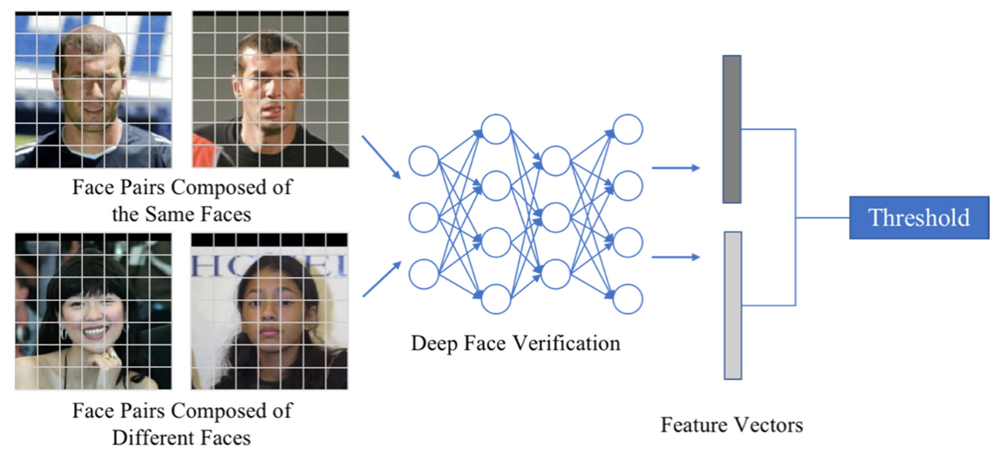
3.1. Face Recognition and Evaluation Matrix

We used a uniform evaluation metric to measure whether a face pair matched or not. A positive sample pair is a matched face pair with the same identity; a negative sample pair is a mismatched face pair. To evaluate the performance of the face recognition model, the following concepts are introduced.

The True Positive Rate (TPR) is calculated as follows:

$$TPR=\frac{TP}{TP+FN}$$

(3)

where TP indicates the matching face pair and is correctly predicted as a matching face pair, and FN means a matching face pair and is incorrectly predicted as a mismatched face pair. TPR is the probability of correctly predicted positive samples to all positive samples, which is the probability of correctly predicted matched face pairs to all matched face pairs.

The False Positive Rate (FPR) is calculated as follows:

$$FPR=\frac{FP}{FP+TN}$$

(4)

where FP denotes a face pair whose true label is mismatched and is incorrectly predicted as a matched face pair. TN denotes a face pair whose true label is mismatched and is correctly predicted as a mismatched face pair. FPR is the probability that the incorrectly predicted negative samples account for all negative samples, and in the face recognition scenario is the probability that the incorrectly predicted mismatched face pairs account for all mismatched face pairs.

Therefore, the accuracy rate (Acc) of the face recognition model is calculated as follows:

$$Acc=\frac{TP+TN}{TP+FN+TN+FP}$$

(5)

That is, the accuracy of the face recognition model is the ratio of the number of correctly predicted face pairs to the total number of face pairs. Meanwhile, we chose five face recognition models with different network architectures for validation. These networks are described in the following sections.

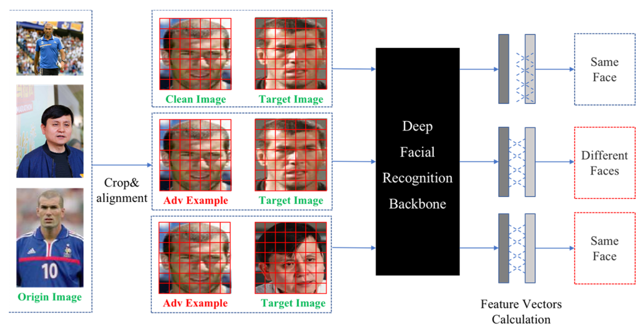
3.2. Adversarial Attacks against Faces

The adversarial attacks are classified into non-targeted attacks and targeted attacks. An intuitive way to do this is to set a threshold. When the distance between two faces and this threshold is compared, if the result is less than the threshold, the two faces are from the same person and vice versa. This is obviously more difficult for the FRS to mistake the target face for another designated one [18].

Suppose that for input $x$, the true label $f\left(x\right)=y$ is output by the classification model $f$. The purpose of the adversarial attack is to generate an adversarial example $x^{adv}$ by adding a small perturbation, and there exists ${\left|\left|x^{adv}-x\right|\right|}_p\le \epsilon$, where $p$ can be 0, 1, 2, ∞. For the non-targeted attack, the generated adversarial example makes $f\left(x^{adv}\right)\ne y$ and the results of the classifier were different from the original label; for the targeted attack, it makes $f\left(x^{adv}\right)\ne y^{*}$, where $y^{*}\ne y$, a previously defined specific class.

3.3. Evaluation Indices of Attack

Our goal is to generate adversarial patches to deceive FRS within a small area of the human face. The patch is generated by optimizing the pixels in the area, changing the distance between pairs of faces. The smaller the patch, the less likely it is to be detected by defenders. We explain the process of generating these patches.

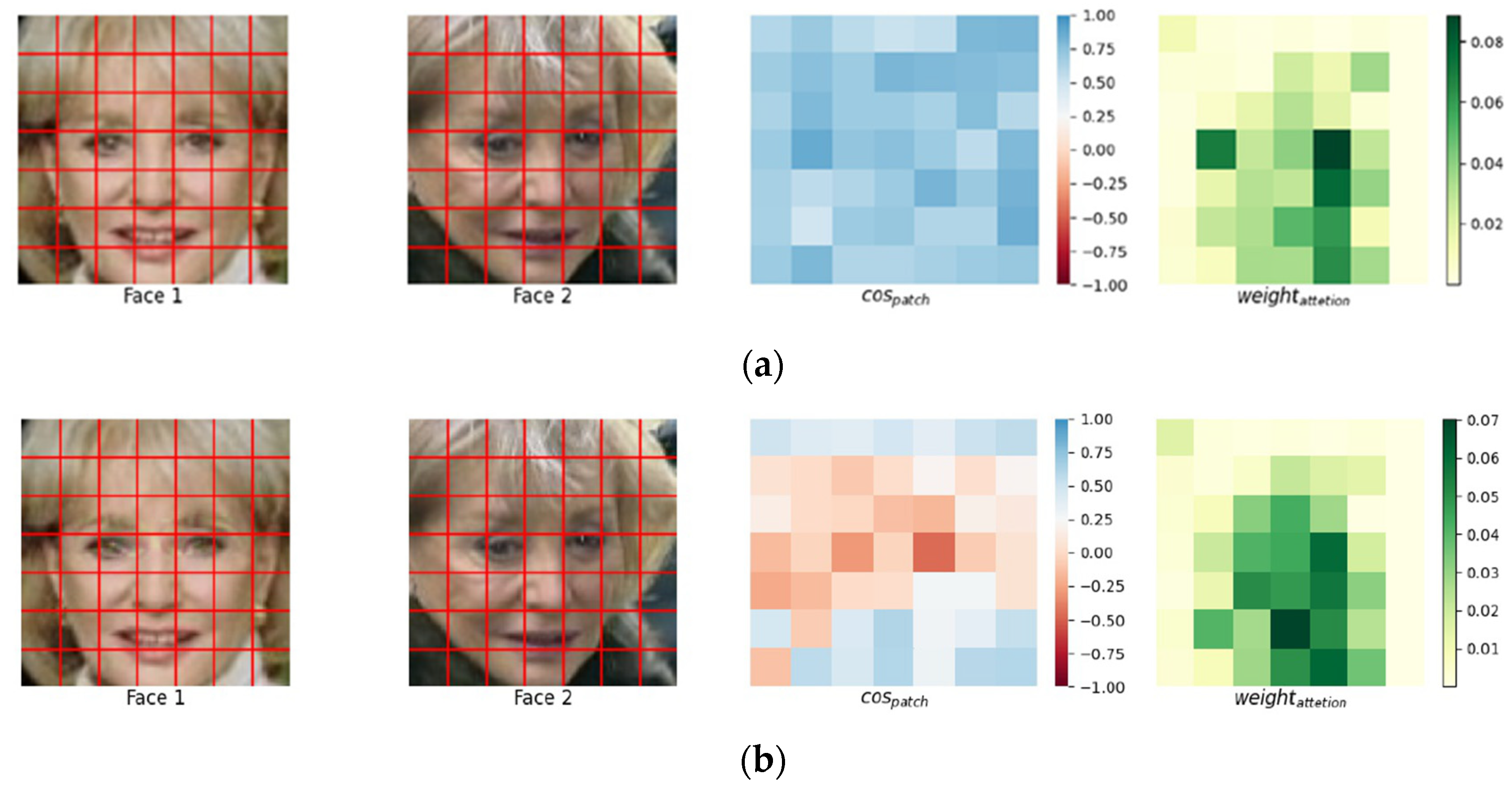
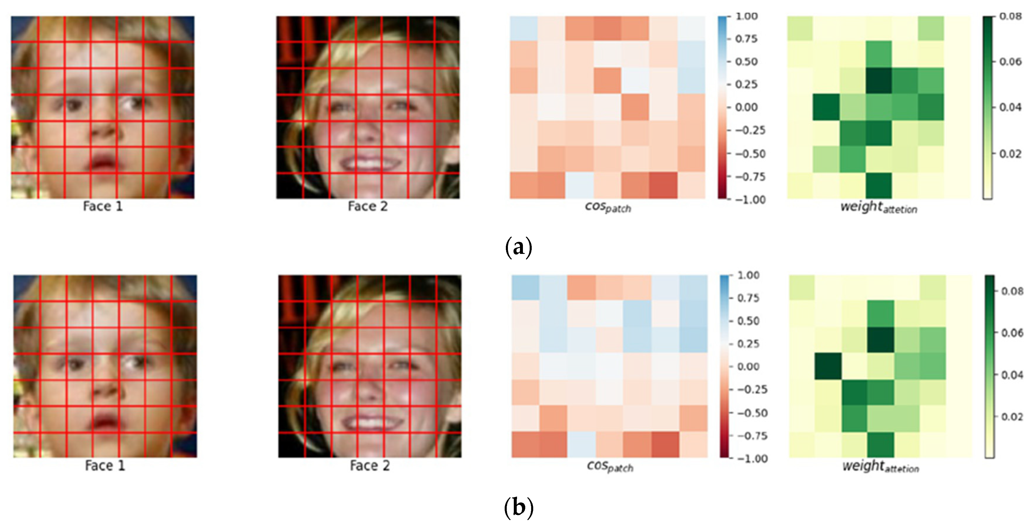
• Cosine Similarity is calculated by the cosine of the angle between two vectors, given as vector $X$ and vector $Y$, and their cosine similarity is calculated as follows.

  $$\cos \left(X,Y\right)=\frac{X\cdot Y}{\parallel X\parallel \parallel Y\parallel }=\frac{{\sum }_{i=1}^n{X}_i{Y}_i}{\sqrt{{\sum }_{i=1}^n{X}_i^2}\sqrt{{\sum }_{i=1}^n{Y}_i^2}}$$

  (6)

  where $X_i$ and $Y_i$ are the individual elements of vector $X$ and vector $Y$, respectively. The cosine similarity takes values in the range [–1, 1], and the closer the value is to 1, the closer the orientation of these two vectors (i.e., the more similar the face feature vectors). Cosine similarity can visually measure the similarity between the adversarial example and the clean image.
• Total variation (TV) [19], as a regular term loss function, reduces the variability of neighboring pixels and makes the perturbation smoother. Additionally, since perturbation smoothness is a prerequisite property for physical realizability against attacks, this lays some groundwork for future physical realizability [18]. Given a perturbation noise $r$, $r_{i,j}$ is the pixel where the perturbation $r$ is located at coordinate $\left(i,j\right)$. The $TV\left(r\right)$ value is smaller when the neighboring pixels are closer (i.e., the smoother the perturbation, and vice versa). The TV is calculated as follows:

  $$TV\left(r\right)={\displaystyle \sum }_{i,j}{\left({\left(r_{i,j}-r_{i+1,j}\right)}^2+{\left(r_{i,j}-r_{i,j+1}\right)}^2\right)}^{\frac{1}{2}}$$

  (7)
• We used the $L_2$ constraints to measure the difference between the original image and the adversarial example. $L_2$ is used as a loss function to control the range of perturbed noise. In the application scenario of attacking, it can be intuitively interpreted as whether the modified pixels will attract human attention.

Given vector $\mathrm{X}$ and vector $\mathrm{Y}$, their $L_2$ distances (i.e., Euclidean distances) can be calculated as follows:

$$\parallel \mathrm{X},\mathrm{Y}{\parallel }_2=\sqrt{{\displaystyle \sum }_i^n{\left(x_i-y_i\right)}^2}$$

(8)

where $x_i$ and $y_i$ are the elements of the input vector $\mathrm{X}$ and the output vector $\mathrm{Y}$, respectively. The larger the $L_2$ distance between the two vectors, the greater their difference.

4. Our Method

4.1. Configurations for Face Adversarial Attack

After the image preprocessing, we extracted the features from the two face images and calculated their distance. For the input face image $x$, the face recognition model $f$ extracted the features. For the input face pairs $\{x_1, x_2\}$, the face feature vector $f\left(x_1\right)$ and $f\left(x_2\right)$ were mapped to 512-dimensional feature vectors, respectively.

Therefore, we compared the distance of $f\left(x_1\right)$ and $f\left(x_2\right)$ with the specified threshold to determine whether the face pair matched or not. We calculated the angular distance by cosine similarity, which is as follows.

$$Similarity=\cos \left(f\left(x_1\right), f\left(x_2\right)\right)$$

(9)

$$D\left(f\left(x_1\right), f\left(x_2\right)\right)=\frac{\mathit{arccos}\left(Similarity\right)}{\pi }$$

(10)

where $\cos \left(·,·\right)$ is the cosine similarity of the feature vector of the face pair in the range of [−1, 1]. Therefore, $D\left(f\left(x_1\right), f\left(x_2\right)\right)$, based on the cosine similarity, ranged from [0, 1]. The closer the distance is to 0, the more similar the face feature vector and the more likely the face pair is matched, and vice versa. Equation (11) is used to predict the matching result of the face pair.

$$C\left(x_1, x_2\right)=\mathbb{I}\left(D\left(f\left(x_1\right), f\left(x_2\right)\right)<threshold\right)$$

(11)

where $\mathbb{I}(·)$ is the indicator function; the threshold is the baseline of the detection model that is different depending on the model used. $C\left(·,·\right)$ outputs the matching result, if $C=1$, the face pair is matched; if $C=0$, the face pair is not matched. A unified attack model is established based on the $\mathbb{I}(·)$ indicator function to implement targeted and non-targeted attacks. The flow of face pair recognition based on the threshold comparison is shown in Figure 3.

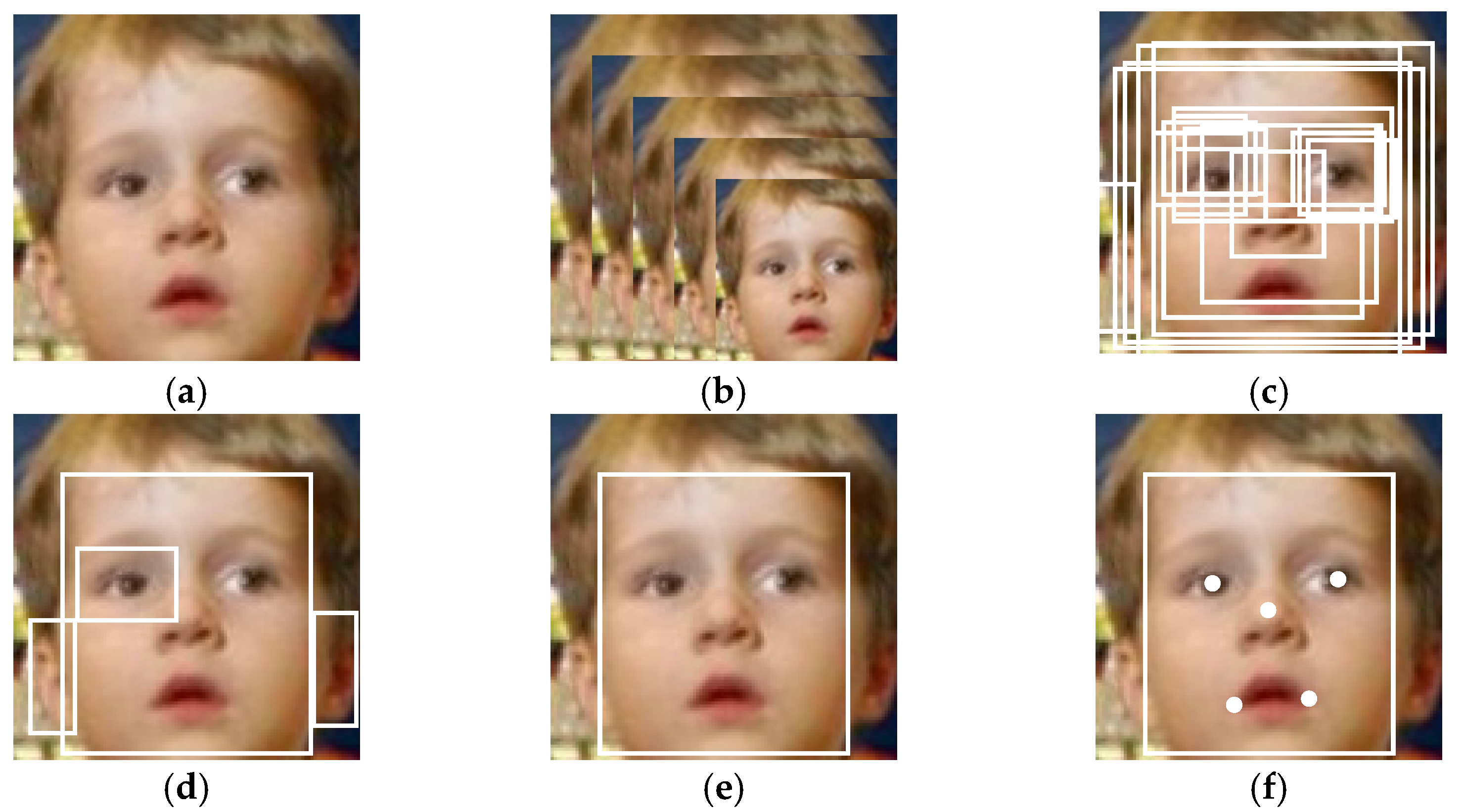
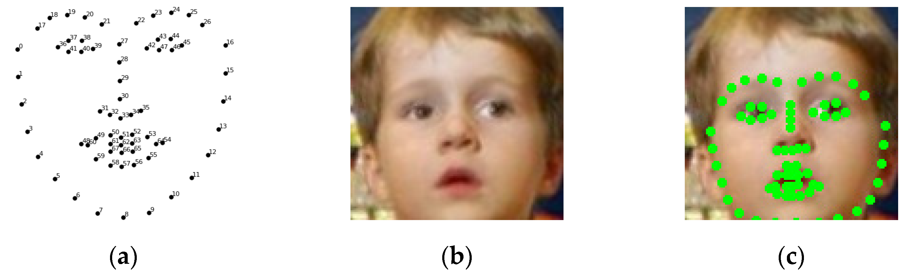
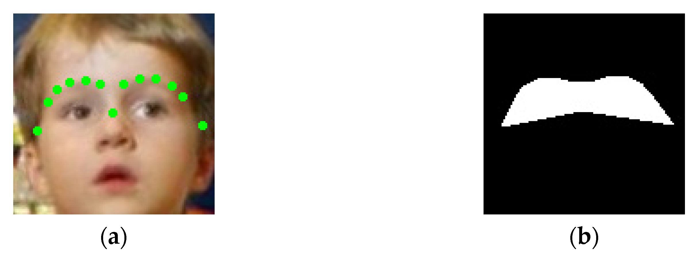
4.2. Local Area Mask Generation

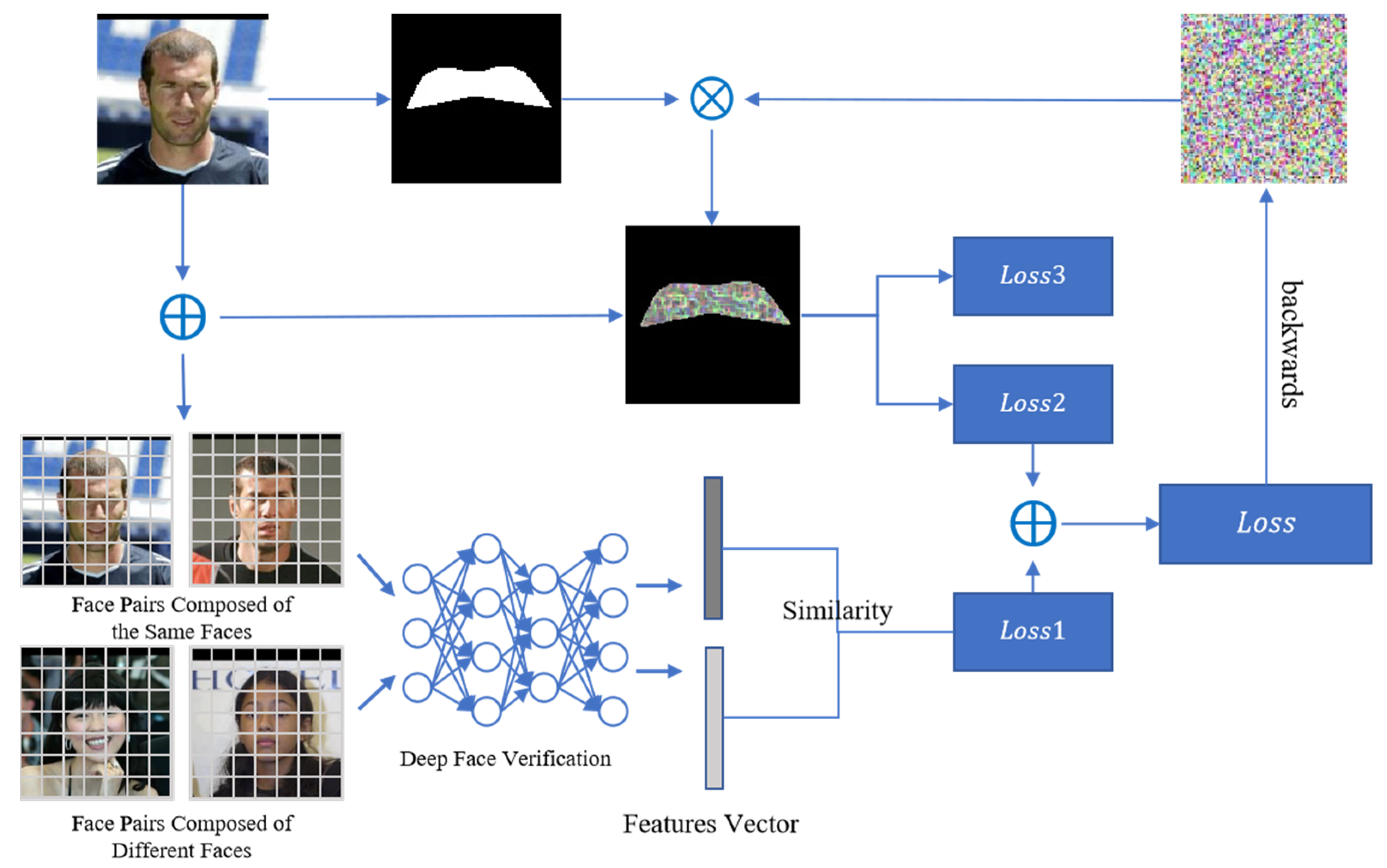
The human eye region contains critical semantic information despite its small area [23]. The local region matrix is generated according to the human eye position as the range of constraint against adversarial perturbance. Due to various poses, illumination, and occlusions, we applied a deeply cascaded multitasking framework to integrate face detection and alignment through multitasking learning. First, since images have different sizes, the key points of the extracted face were affined to the unit space using affine transformation to unify the size and coordinate system. The detection and alignment of faces were accomplished by building a multi-level CNN structure containing three stages. Candidate windows will be quickly generated by a shallow CNN. Then, the windows were optimized by more complex CNNs to discard a large number of non-facial windows. Finally, it refines the results. by using a more powerful CNN and outputs the facial marker positions.

The algorithm flow is shown in Figure 4. In Figure 4b, for a given image, we first adjusted it to different scales to construct the image pyramid. In Figure 4c, we referred to the method in [29] to obtain the candidate windows and their bounding box regression vectors. The estimated bounding box regression vectors were then used to calibrate the candidate boxes; in Figure 4d, we used non-maximal suppression (NMS) to merge the highly overlapping candidate objects. In Figure 4e, all candidate frames were used as input to the CNN of the optimization network, which further discarded a large number of incorrect candidate frames, calibrated them using bounding box regression, and merged the NMS candidate frames. Finally, Figure 4f shows the CNN-based classification network that generated a more detailed description of the faces and outputs the critical facial positions.

Pixels are randomly sampled within the range of key points as the corresponding feature pixel [29]. The feature pixels select the closest initial key point as the anchor and calculate the deviation. The coordinate system of the current pixel after rotation, transformation, and scaling should be close to the initial key point. It acts on the deviation and adds its own position information to obtain the feature pixel of the current key point. Then, we constructed the residual tree and calculated the deviation of the current key point from the target key point. We split the sample and updated the current key point position based on the average residual of the sample. Back to the previous step, it reselected the feature key points, fit the next residual tree, and finally combined the results of all residual trees to obtain the key point locations. According to the default settings, the coordinates of the points 0, 28, 16, 26–17 in the image for the human eye area are shown in Figure 5.

We located the human eye region based on the key points of the detected eye in the image and drew the mask against the attacked region. The range of pixel values in the generated mask image was normalized to [0.0, 1.0] to generate a binary-valued mask matrix. This is shown in Figure 6.

We generated adversarial examples combining the eye region matrix and full face region, respectively, to test the effect of the attacks. Figure 7a shows the clean image used for testing while Figure 7b shows the visualization of the perturbation based on the eye region and the full-face region. Figure 7c is the adversarial example. After testing, both images could successfully deceive the face detector. The adversarial perturbation generated based on the human eye region accounted for 17.8% of the total pixels, while the number of pixels of the adversarial perturbation generated based on the whole face accounted for 81.3% of the image.

4.3. Loss Functions

As above-mentioned, this algorithm optimizes the $C\left(x,x^{adv}\right)$ function in the local region. For the targeted attack and non-targeted attack, the relationship between the clean face image $x$ and the three target images $x^{tar}$ and the adversarial example image $x^{adv}$ was compared.

(1)

For the non-targeted attack, an adversarial example $x^{adv}$ was generated for the input image $x$ so that the difference between them was as large as possible. When the difference was larger than the threshold value calculated by the deep detection model, the attack was successful; on the other hand, for the targeted attack, the generated adversarial example $x^{adv}$ needed to be as similar as possible to the target image $x^{tar}$. The loss function $ℒos{s}_1$ is shown as Equation (12).

$$ℒos{s}_1=\alpha ·\cos \left(f\left(x\right),f\left(x^{adv}\right)\right)-\left(1-\mathsf{\alpha }\right)·\cos \left(f\left(x^{adv}\right),f\left(x^{tar}\right)\right)$$

(12)

where $cos\left(·,·\right)$ is the cosine similarity of the feature vector calculated by Equation (10); $\alpha$ takes the value of 0 or 1, representing the non-targeted attack and targeted attack, respectively.

(2)

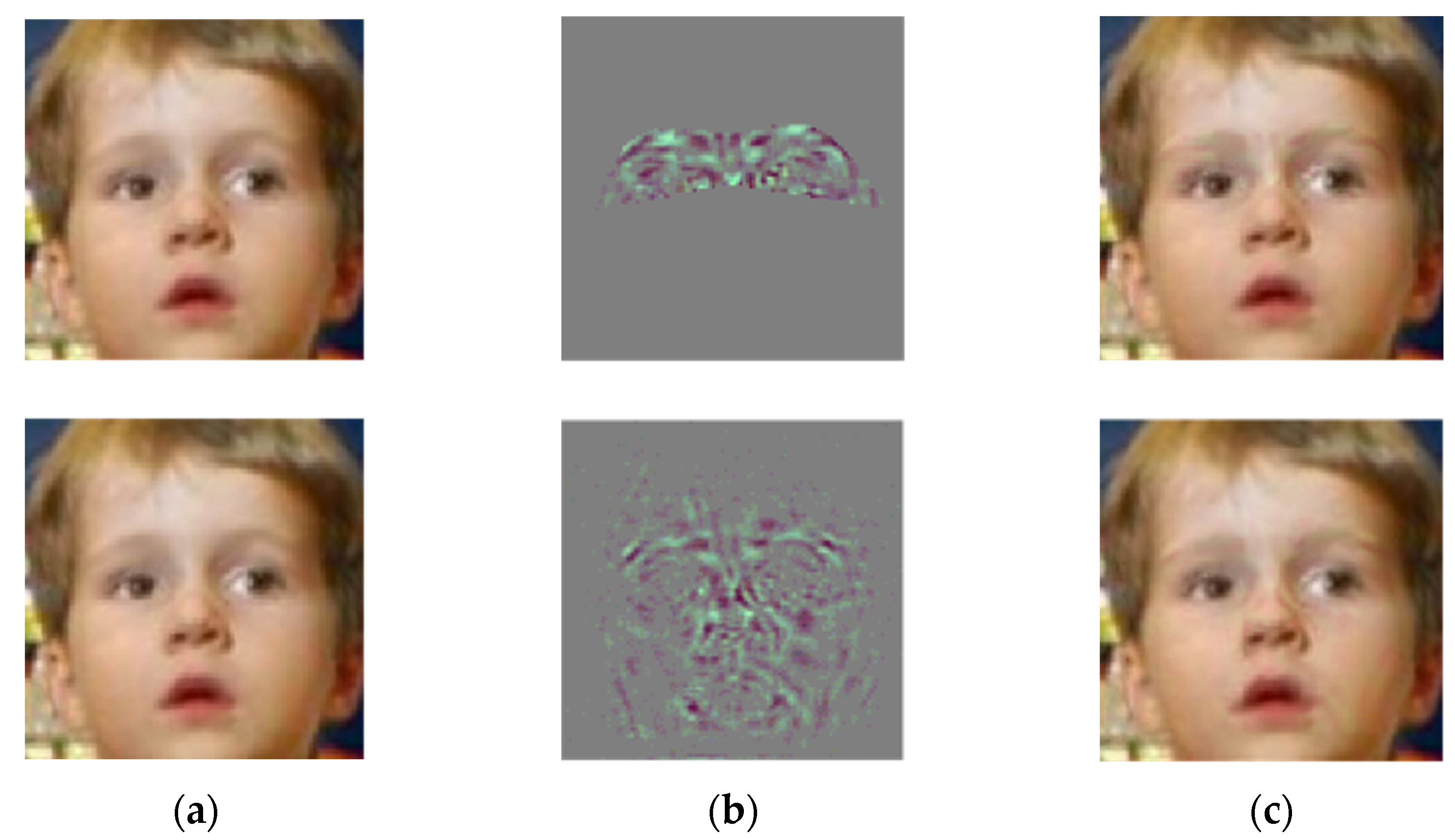
The perturbation size is constrained by the $L_2$ norm, thus ensuring that the visibility of the perturbation is kept within a certain range when an effective attack is implemented. The loss function in this section constrains the perturbation after the restriction as follows.

$$ℒos{s}_2=L_2\left(mask\odot r\right)$$

(13)

where $r$ is the perturbation. The mask is that generated from the first face image of the face pair to restrict the perturbation region. It is a [0, 1] matrix scaled to the same size as the image. The ⨀ symbol indicates the dot product operation between the elements.

(3)

The TV is used to improve the smoothness of the perturbation through Equation (14), and the loss function of this part also deals with the perturbation after restriction, as follows.

$$ℒos{s}_3=TV\left(mask\odot r\right)$$

(14)

In summary, for the above targeted and non-targeted attacks, the loss function is minimized by solving the following optimization problem of Equation (15), which can generate the final adversarial perturbation $r:$

$$\underset{r}{min}ℒ\mathit{oss}=\underset{r}{min}\left({\lambda }_1ℒ{\mathit{oss}}_1+{\lambda }_2ℒ{\mathit{oss}}_2+{\lambda }_3ℒ{\mathrm{oss}}_3\right)$$

(15)

The hyperparameters ${\lambda }_1$, ${\lambda }_2$, and ${\lambda }_3$ are used to control the relative weights of the perturbation losses. The correlation coefficients of the two regular term loss functions $ℒos{s}_2$ and $ℒos{s}_3$ are gradually reduced as the number of iterations increases.

4.4. Momentum-Based Optimization Algorithms

To solve the optimization problem above, the adversarial perturbation is optimized by using an iterative gradient descent method to minimize the objective function. A momentum parameter superimposes in the gradient direction and dynamically stabilizes update directions in each iteration step [12].

In the updating process, due to the different iterations of updating for different scenes, we divided the updating process into several stages, and the learning rate of different stages gradually decreased. The gradient is calculated as follows.Meanwhile, the learning rate ${\alpha }_{\Delta t}$ is changed according to the number of iterations $it$ and stages $st$.

$$\begin{gathered} grad=\beta ·m_i+\frac{{\nabla }_xℒ\mathit{oss}\left(x^{adv},y\right)}{{\left|\left|{\nabla }_xℒ\mathit{oss}\left(x^{adv},y\right)\right|\right|}_1} \\ {m}_{i+1}=grad \\ {r}_{t+1}=r_t-{\alpha }_{\Delta i}\ast grad \\ {\alpha }_{\Delta i}={\left(\frac{it}{st}\right)}^i{a}_{\Delta \left(i-1\right)}+a_{\Delta \left(i-1\right)} \end{gathered}$$

(16)

where $\left|\right|{\nabla }_xℒ\mathit{oss}\left(x^{adv},y\right)|{|}_1$ is the regularized representation of the gradient of ${\nabla }_xℒ\mathit{oss}\left(x^{adv},y\right)$. The parameter $\beta$ is the decay factor, adjusting for the influence of momentum on the gradient calculation. $r_t$ is the adversarial perturbation generated in the $t$ iteration. The parameter ${\alpha }_{\Delta t}$ is dynamically adjusted and is related to the iterations $it$ and the current stages $st$. If $it$ is high, then * can be set bigger. As $it$ increases, $st$ will become smaller.

$$x_{t+1}^{adv}=cli{p}_{x,\epsilon }\left(x+mask\odot r_{t+1}\right)$$

(17)

where $cli{p}_{x,\epsilon }(·)$ serves to restrict the adversarial examples after superimposed perturbation to a reasonable range (after normalization) of [−1, 1] at the end of each iteration.

The final elaborate perturbation is processed and added to the original face image so that the final adversarial example is generated by restricting the perturbation to a reasonable range of [0, 255] using $cli{p}_{x,\epsilon }(·)$. The process is shown in Figure 8.

Figure 8 shows that the feature vectors are first extracted from the aligned faces. The attack region is mapped by keypoint detection and the adversarial perturbation information is generated based on this region. The local aggressive perturbation is obtained through the optimization of the loss functions. This perturbation information can effectively mislead FRS.

5. Experiments

5.1. Datasets

In this paper, we used CASIA WebFace [7] as the training dataset. All of the pictures are from movie websites and vary in light and angle. In order to verify the effect of the algorithm on different datasets, we choose LFW [22] as our test dataset. It provides 6000 test face pairs, of which 3000 are matched pairs and 3000 are mismatched pairs.

For face detection and alignment, MTCNN [30,31,32,33,34] was used to uniformly crop the images to 112 × 112. Experimentally, there were 500 pairs of matched faces with the same identity for non-targeted attacks and 500 pairs of unmatched faces with different identities for targeted attacks.

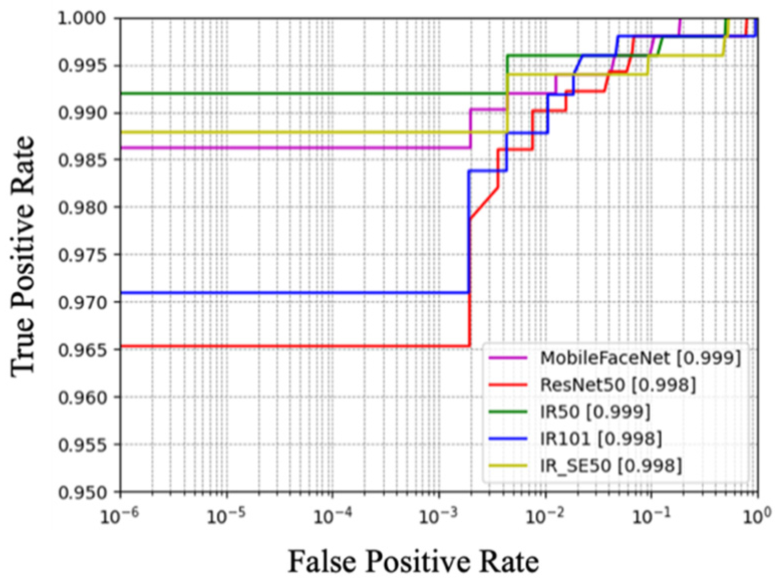
5.2. Performance Evaluation for Face Recognition Models

Five mainstream pre-trained face recognition models were used for comparison, namely ResNet50-IR (IR50) [31], ResNet101-IR (IR101) [32], SEResNet50-IR (IR-SE50) [33], MobileFaceNet [8], and ResNet50 [33]. In order to show the success rate of adversarial attacks more intuitively, the metrics were the True Accept Rate (TAR) and False Accept Rate (FAR) [20]. Given a face pair $\left(x_1,x_2\right)$, let the matched face pair be $P_s$ and the unmatched face pair be $P_d$. Given a threshold, the calculation of TAR and FAR is as follows.

$$TA=\left\{\begin{array}{c}\left({\mathit{x}}_1, {\mathit{x}}_2\right)\in P_s, \\ \mathrm{with} D\left(f\left({\mathit{x}}_1\right), f\left({\mathit{x}}_2\right)\right)<threshold\end{array}\right\}$$

(18)

$$FA=\left\{\begin{array}{c}\left({\mathit{x}}_1, {\mathit{x}}_2\right)\in P_d, \\ \mathrm{with} D\left(f\left({\mathit{x}}_1\right), f\left({\mathit{x}}_2\right)\right)<threshold\end{array}\right\}$$

(19)

$$TAR=\frac{\left|TA\right|}{\left|P_s\right|}$$

(20)

$$FAR=\frac{\left|FA\right|}{\left|P_d\right|}$$

(21)

where $\left|TA\right|$ is the number of all matched pairs whose distance is less than the threshold; $\left|P_s\right|$ is the number of all matched pairs; $\left|FA\right|$ is the number of all unmatched pairs whose distance is less than the threshold; and $\left|P_d\right|$ is the number of all unmatched face pairs.

Different models will have different thresholds that can objectively reflect the success rate of the attack. Accordingly, the threshold was determined according to different values of $\mathit{FAR}$, and was chosen when $\mathit{FAR}=1\times {10}^{-2}$ or $1\times {10}^{-3}$. We traversed the range of thresholds and used the 10-fold cross-validation method to find the threshold closest to the target FAR.

As shown in Figure 9, the TPR of each model (i.e., the proportion of correctly predicted matched face pairs to all unmatched face pairs) was maintained above 96.5% when $\mathit{FAR}=1\times {10}^{-6}$. When $\mathit{FAR}=1\times {10}^{-2}$, the TPR reached more than 98.5%. This indicates that the performance of these backbone network models had excellent performance.

The test results of the five models on the LFW at a FAR of about 0.01 are shown in

Table 1. The TAR and corresponding thresholds for different models.

Models	TAR (%)	FAR	Threshold	Sim-Threshold
IR50	99.596	0.00995	0.43326	0.20814
IR101	98.984	0.01259	0.41311	0.26960
IR-SE50	99.396	0.01025	0.42920	0.22060
ResNet50	99.596	0.00836	0.45207	0.15001
MobileFaceNet	99.196	0.01076	0.43763	0.19469

. The value of TAR@FAR = 0.01 (i.e., the probability of correctly identifying matching face pairs when the FAR is close to 0.01) was maintained at more than 98.9%.

5.3. Attack Method Evaluation Indicators

The accuracy of a face recognition model intuitively reflects the predictive ability of the model. The attack success rate (ASR) is calculated as follows:

$$ASR=1-Acc$$

(22)

The higher the ASR, the more vulnerable the model is to adversarial attacks; the lower the ASR, the more robust the model is to adversarial attacks and is able to withstand a certain degree of adversarial attacks.

In order to evaluate the magnitude of the difference between the generated adversarial example and the original face image after the attack, this experiment used the peak signal-to-noise ratio (PSNR), and structural similarity (SSIM) [34], which are two metrics to measure the image quality of the adversarial example.

The PSNR is defined and calculated by the mean squared error (MSE). The following equation calculates the PSNR for a given image $I$.

$$PSNR=20\cdot lo{g}_{10}\left(MA{X}_I\right)-10\cdot lo{g}_{10}\left(MSE\right)$$

(23)

where $MA{X}_I$ is the maximum pixel value of the image; $MSE$ is the mean square error. The larger the PSNR, the less distortion and the better quality of the adversarial example [3].

Considering human intuition, we adopted the evaluation index of structural similarity (SSIM), which takes into account the three factors of brightness, contrast, and structure. Given images $x$ and $y$ with the same dimensions, the structural similarity is calculated as follows.

$$SSIM\left(x,y\right)=\frac{\left(2{\mu }_x{\mu }_y+c_1\right)\left(2{\sigma }_{xy}+c_2\right)}{\left({\mu }_x^2+{\mu }_y^2+c_1\right)\left({\sigma }_x^2+{\sigma }_y^2+c_2\right)}$$

(24)

Among them, ${\mu }_x$, ${\mu }_y$ are the mean values of image $x,y$; ${\sigma }_x^2, {\sigma }_y^2$ are the variance of image $x$, $y$; ${\sigma }_{xy}$ is the covariance, and $c_1$ and $c_2$ are used to maintain stability. SSIM takes values in the range of [−1, 1], and the closer the value is to 1, the higher the structural similarity between the adversarial example and the original image. To a certain extent, it can indicate the more imperceptible the perturbation applied to the adversarial example is to humans.

5.4. Adversarial Attack within Human Eye Area

5.4.1. Non-Targeted Attacks based on Eye Area

A schematic diagram of the non-targeted attack is shown in Figure 10. The first column shows the face pair before the attack. To the human eye, there is no difference between the second image in Figure 10a,b, and the second image in Figure 10b is the adversarial example.

$weigh{t}_{attetion}$ in the fourth column indicates the attention of the model, where the darker color indicates that the model paid more attention to the area. It can be seen that there was no significant change in the attention hotspots before and after the attack. In the third column, the xCos [35] module visualizes the face pairs before and after the attack and visualizes the changes in the images from the perspective of the neural network parameters. The bluer color in the similarity plot $co{s}_{patch}$ indicates that they are more similar, and the redder color indicates that they are less similar. It can be seen that the face pairs changed dramatically after the attack.

5.4.2. Targeted Attacks Based on Eye Area

The purpose of the targeted attack is to deceive the deep detection model into misidentifying another specific face from the original image. As shown in Figure 11a, the similarity graph of the face pair before the attack had a large number of red grids, indicating that this pair was very dissimilar and was a mismatched face pair, while the model’s attention focused on the eye area in the middle of the face. The first image in Figure 11b is the generated adversarial example; the second image is the target image. Intuitively, the first images in Figure 11a,b are exactly the same. This is also reflected in the attention map. However, for the face recognition model, the grid of the eye region in $co{s}_{patch}$ mostly changed to blue, and 43% of the regions changed from yellow to blue. This indicates that the image change affected the classification of deep model.

5.4.3. Quantitative Comparison of Different Attack Models

To verify the effectiveness of the algorithm, we selected 500 faces for targeted and non-targeted attacks. Furthermore, each model has a different threshold for the best performance. The attack success rates of different attack models are shown in

Table 2. The accuracy and success rates of different models under the specified thresholds.

Models	ACC (%)	Targeted-ASR (%)	Non-Targeted-ASR (%)	Threshold
IR50	98.2	90.4	99.2	0.43326
IR101	94.7	96.2	98.6	0.41311
IR-SE50	92.6	92.2	98.8	0.42920
ResNet50	94.5	93.8	99.4	0.45207
MobileFaceNet	96.6	91.4	99.2	0.43763

.

Our method was compared with the traditional adversarial algorithms. With a high success rate, we compared the differences between the adversarial examples and the original images, and the evaluated metrics included the image quality of the adversarial examples, the calculated average PSNR and SSIM. The perturbations of the adversarial examples generated by our algorithm for different deep detection models were counted. A PSNR greater than 40 indicates that the image distortion was small; the closer the SSIM takes the value of 1, the closer the adversarial example is to the original image. The comparison results are shown in

Table 3. Average PSNR, SSIN, and the perturbed parameters for different models.

Models	Targeted-PSNR	Targeted-SSIM	Targeted-L2	Non-Targeted-PSNR	Non-Targeted-SSIM	Non-Targeted-L2
IR50	43.69864	0.99358	0.71112	39.19224	0.98557	1.29420
IR101	43.68891	0.99379	0.71556	42.37390	0.99232	0.84162
IR-SE50	43.46344	0.99345	0.76280	39.95576	0.98470	1.22338
ResNet50	45.51955	0.99531	0.58352	40.89765	0.98938	1.09996
MobileFaceNet	43.82034	0.99395	0.72392	41.36429	0.98954	1.04512

.

As shown in Table 3, for different attacks, the PSNR of all models was above 40 dB and the SSIM was above 0.98, indicating that the image distortion was very small and the perturbations were imperceptible to humans; on the other hand, the perturbations generated by the targeted attack was much lower than that of the non-targeted attack. The momentum in this algorithm was updated toward the target image due to the directed output of the image. Therefore, the adversarial example generation algorithm was also guided to optimize in the direction of the specific objects.

5.4.4. Comparison of Adversarial Example Algorithms

In this paper, the validation dataset covered 40 different categories. These categories can be correctly classified by the MobileFaceNet model (Top-1 correct); we also selected ArcFace [3] and SphereFace [21] face recognition models for testing. ArcFace uses IR101 as the network structure and has 99.8% accuracy in the LFW test set; SphereFace’s network structure removes the BN module, which differs significantly from the ResNet50 residual network, with 99.5% accuracy in the LFW test set. We selected a variety of typical adversarial example algorithms FGSM [10], I-FGSM [11] algorithms, and the face-specific attack method AdvGlasses [18], AdvHat [19], and our algorithm (AdvLocFace) for cross-testing. The comparison results are shown in

Table 4. Accuracy and success rates of different algorithms.

Models	Attack Method	ResNet50	MobileFaceNet	SphereFace	ArcFace
ResNet50	FGSM	77.00%	34.81%	31.88%	30.26%
	I-FGSM	100.00%	24.41%	21.76%	18.82%
	AdvGlasses	100.00%	51.05%	48.02%	40.58%
	AdvHat	97.80%	52.92%	44.87%	44.24%
	AdvLocFace	99.10%	57.15%	51.35%	59.00%
MobileFaceNet	FGSM	39.99%	67.67%	27.83%	29.04%
	I-FGSM	38.86%	100.00%	24.59%	20.75%
	AdvGlasses	69.39%	100.00%	46.06%	45.64%
	AdvHat	77.61%	97.90%	46.29%	37.38%
	AdvLocFace	61.62%	99.20%	52.76%	40.92%
SphereFace	FGSM	38.55%	32.34%	59.20%	28.74%
	I-FGSM	41.94%	33.37%	99.88%	25.91%
	AdvGlasses	76.59%	65.61%	99.58%	53.53%
	AdvHat	68.03%	54.06%	93.91%	64.16%
	AdvLocFace	62.96%	58.90%	96.65%	67.91%
ArcFace	FGSM	37.01%	33.58%	30.76%	75.19%
	I-FGSM	31.56%	25.65%	21.96%	98.67%
	AdvGlasses	57.88%	52.43%	50.20%	97.35%
	AdvHat	68.61%	65.90%	63.19%	100.00%
	AdvLocFace	73.24%	70.64%	70.57%	100.00%

.

In Table 4, the diagonal lines are white-box attack settings. I-FGSM improved the success rate of white-box attacks by increasing the iterative process, but reduced the mobility of the attack method due to the overfitting of the perturbation. The AdvHat algorithm is an advanced physical attack method that attacks realistic attacks by pasting stickers on the hat, and it is easy to replicate this attack. The optimization process, based on the consideration of pixel smoothing and color printability, limits the effect of mobility in digital attacks. AdvLocFace, with the best threshold for similar models based on the base model of training, obtained a more stable success rate of black-box attacks. For network models with different structures and different training data, the attack success rate decreased significantly.

6. Conclusions

This paper proposed a face adversarial example generation algorithm based on local regions. The algorithm uses the principle of a face recognition system to build a local area containing key features and generates momentum-based adversarial examples. This algorithm is a typical white-box attack method but still achieves good results in the black-box attack scenario.

Compared with the traditional adversarial attack method, the adversarial perturbance generated by our method only needs to cover a small part of the original image. Because the region contains the key features of the face, it can successfully mislead the face recognition system. In addition, the generated adversarial example is patch-like, which is highly similar to the original image and therefore more inconspicuous. Our algorithm can selectively attack any target in the image, so it can be extended to attack other types of images. the experiments show that the proposed algorithm can effectively balance the modified pixel area and attack successfully, achieving good transferability.

References

1. Taigman, Y.; Yang, M.; Ranzato, M.A.; Wolf, L. DeepFace: Closing the gap to human-level performance in face verification. In Proceedings of the IEEE Conference on Computer Vision and Pattern Recognition, Columbus, OH, USA, 23–28 June 2014. [Google Scholar]
2. Taigman, Y.; Yang, M.; Ranzato, M.A.; Wolf, L. Web-scale training for face identification. In Proceedings of the IEEE Conference on Computer Vision and Pattern Recognition, Boston, MA, USA, 7–12 June 2015. [Google Scholar]
3. Deng, J.; Guo, J.; Xue, N.; Zafeiriou, S. Arcface: Additive angular margin loss for deep face recognition. In Proceedings of the IEEE/CVF Conference on Computer Vision and Pattern Recognition, Long Beach, CA, USA, 16–20 June 2019; pp. 4690–4699. [Google Scholar]
4. Wang, H.; Wang, Y.; Zhou, Z.; Ji, X.; Gong, D.; Zhou, J.; Li, Z.; Liu, W. Cosface: Large margin cosine loss for deep face recognition. In Proceedings of the IEEE Conference on Computer Vision and Pattern Recognition, Salt Lake City, UT, USA, 18–22 June 2018. [Google Scholar]
5. Florian, S.; Kalenichenko, D.; Philbin, J. Facenet: A unified embedding for face recognition and clustering. In Proceedings of the IEEE Conference on Computer Vision and Pattern Recognition, Boston, MA, USA, 7–12 June 2015. [Google Scholar]
6. Tianyue, Z.; Deng, W.; Hu, J. Cross-age lfw: A database for studying cross-age face recognition in unconstrained environments. arXiv 2017, arXiv:1708.08197. [Google Scholar]
7. Yi, D.; Lei, Z.; Liao, S.; Li, S.Z. Learning Face Representation from Scratch. arXiv 2014, arXiv:1411.7923. [Google Scholar]
8. Chen, S.; Liu, Y.; Gao, X.; Han, Z. MobileFaceNets: Efficient CNNs for Accurate Real-time Face Verification on Mobile Devices. In Proceedings of the Chinese Conference on Biometric Recognition, Beijing, China, 3–4 December 2018; pp. 428–438. [Google Scholar]
9. Thys, S.; Van Ranst, W.; Goedeme, T. Fooling automated surveillance cameras: Adversarial patches to attack person detection. In Proceedings of the 2019 IEEE/CVF Conference on Computer Vision and Pattern Recognition Workshops (CVPRW), Long Beach, CA, USA, 16–17 June 2019; pp. 49–55. [Google Scholar]
10. Szegedy, C.; Zaremba, W.; Sutskever, I.; Bruna, J.; Erhan, D.; Goodfellow, I.; Fergus, R. Intriguing properties of neural networks. arXiv 2014, arXiv:1312.6199. [Google Scholar]
11. Goodfellow, I.J.; Shlens, J.; Szegedy, C. Explaining and harnessing adversarial examples. arXiv 2014, arXiv:1412.6572. Available online: https://arxiv.org/abs/1412.6572 (accessed on 23 October 2022).
12. Dong, Y.; Liao, F.; Pang, T.; Su, H.; Zhu, J.; Hu, X.; Li, J. Boosting Adversarial Attacks with Momentum. In Proceedings of the IEEE Conference on Computer Vision and Pattern Recognition, Salt Lake City, UT, USA, 18–22 June 2018; pp. 9185–9193. [Google Scholar]
13. Carlini, N.; Wagner, D.A. Towards Evaluating the Robustness of Neural Networks. In Proceedings of the 2017 IEEE Symposium on Security and Privacy (SP), San Jose, CA, USA, 22–26 May 2017; pp. 39–57. [Google Scholar]
14. Liu, X.; Yang, H.; Liu, Z.; Song, L.; Chen, Y.; Li, H. DPATCH: An Adversarial Patch Attack on Object Detectors. arXiv 2019, arXiv:1806.02299. [Google Scholar]
15. Kevin, E.; Ivan, E.; Earlence, F.; Bo, L.; Amir, R.; Florian, T.; Atul, P.; Tadayoshi, K.; Dawn, S. Physical Adversarial Examples for Object Detectors. arXiv 2018, arXiv:1807.07769. [Google Scholar]
16. Wu, Z.; Lim, S.; Davis, L.; Goldstein, T. Making an Invisibility Cloak: Real World Adversarial Attacks on Object Detectors. In Proceedings of the 16th European Conference on Computer Vision, Glasgow, UK, 23–28 August 2020. [Google Scholar]
17. Xu, K.; Zhang, G.; Liu, S.; Fan, Q.; Sun, M.; Chen, H.; Chen, P.; Wang, Y.; Lin, X. Evading Real-Time Person Detectors by Adversarial T-shirt. arXiv 2019, arXiv:1910.11099v1. [Google Scholar]
18. Sharif, M.; Bhagavatula, S.; Bauer, L.; Reiter, M.K. Accessorize to a Crime: Real and Stealthy Attacks on State-of-the-Art Face Recognition. In Proceedings of the CCS’16: 2016 ACM SIGSAC Conference on Computer and Communications Security, Vienna, Austria, 24–28 October 2016. [Google Scholar]
19. Komkov, S.; Petiushko, A. AdvHat: Real-world adversarial attack on ArcFace Face ID system. In Proceedings of the 2020 25th International Conference on Pattern Recognition (ICPR), Milan, Italy, 10–15 January 2021. [Google Scholar]
20. Huang, G.B.; Mattar, M.; Berg, T.; Learned-Miller, E. Labeled faces in the wild: A database for studying face recognition in unconstrained environments. In Proceedings of the Workshop on Faces in ‘Real-Life’ Images: Detection, Alignment, and Recognition, Marseille, France, 17 October 2008; pp. 1–11. [Google Scholar]
21. Liu, W.; Wen, Y.; Yu, Z.; Li, M.; Raj, B.; Song, L. Sphereface: Deep hypersphere embedding for face recognition. In Proceedings of the IEEE Conference on Computer Vision and Pattern Recognition, Honolulu, HI, USA, 21–26 July 2017; pp. 212–220. [Google Scholar]
22. Lang, D.; Chen, D.; Shi, R.; He, Y. Attention-Guided Digital Adversarial Patches On Visual Detection. Secur. Commun. Netw. 2021, 2021, 6637936:1–6637936:11. [Google Scholar] [CrossRef]
23. Nguyen, D.; Arora, S.S.; Wu, Y.; Yang, H. Adversarial Light Projection Attacks on Face Recognition Systems: A Feasibility Study. Available online: https://arxiv.org/abs/2003.11145 (accessed on 23 October 2022).
24. Ioffe, S.; Szegedy, C. Batch Normalization: Accelerating Deep Network Training by Reducing Internal Covariate Shift. In Proceedings of the International Conference on Machine Learning, Lille, France, 6–11 July 2015. [Google Scholar]
25. Zolfi, A.; Avidan, S.; Elovici, Y.; Shabtai, A. Adversarial Mask: Real-World Adversarial Attack Against Face Recognition Models. arXiv 2021, arXiv:2111.10759. [Google Scholar]
26. Yin, B.; Wang, W.; Yao, T.; Guo, J.; Kong, Z.; Ding, S.; Li, J.; Liu, C. Adv-Makeup—A New Imperceptible and Transferable Attack on Face Recognition. In Proceedings of the International Joint Conference on Artificial Intelligence, Montreal, QC, Canada, 19–27 August 2021; pp. 1252–1258. [Google Scholar]
27. Xiao, Z.; Gao, X.; Fu, C.; Dong, Y.; Gao, W.; Zhang, X.; Zhou, J.; Zhu, J. Improving transferability of adversarial patches on face recognition with generative models. In Proceedings of the IEEE/CVF Conference on Computer Vision and Pattern Recognition, Virtual, 19–25 June 2021; pp. 11845–11854. [Google Scholar]
28. Parmar, R.; Kuribayashi, M.; Takiwaki, H.; Raval, M.S. On Fooling Facial Recognition Systems using Adversarial Patches. In Proceedings of the 2022 International Joint Conference on Neural Networks, Padova, Italy, 18–23 July 2022; pp. 1–8. [Google Scholar]
29. Jia, S.; Yin, B.; Yao, T.; Ding, S.; Shen, C.; Yang, X.; Ma, C. Adv-Attribute: Inconspicuous and Transferable Adversarial Attack on Face Recognition. arXiv 2022, arXiv:2210.06871. [Google Scholar]
30. Zhang, K.; Zhang, Z.; Li, Z.; Qiao, Y. Joint face detection and alignment using multitask cascaded convolutional networks. IEEE Signal Process. Lett. 2016, 23, 1499–1503. [Google Scholar] [CrossRef] [Green Version]
31. Farfade, S.S.; Saberian, M.J.; Li, L.J. Multi-view Face Detection Using Deep Convolutional Neural Networks. In Proceedings of the 5th ACM on International Conference on Multimedia Retrieval, Shanghai, China, 23–26 June 2015; pp. 643–650. [Google Scholar]
32. He, K.; Zhang, X.; Ren, S.; Sun, J. Deep residual learning for image recognition. In Proceedings of the IEEE Conference on Computer Vision and Pattern Recognition, Las Vegas, NV, USA, 27–30 June 2016; pp. 770–778. [Google Scholar]
33. Hu, J.; Shen, L.; Sun, G. Squeeze-and-excitation networks. In Proceedings of the IEEE Conference on Computer Vision and Pattern Recognition, Salt Lake City, UT, USA, 18–23 June 2018; pp. 7132–7141. [Google Scholar]
34. Huynh-Thu, Q.; Ghanbari, M. Scope of validity of PSNR in image/video quality assessment. Electron. Lett. 2008, 44, 800–801. [Google Scholar] [CrossRef]
35. Lin, Y.S.; Liu, Z.Y.; Chen, Y.A.; Wang, Y.S.; Chang, Y.L.; Hsu, W.H. xCos: An Explainable Cosine Metric for Face Verification Task. ACM Trans. Multimed. Comput. Commun. Appl. 2021, 17, 1–16. [Google Scholar]
Figure 1. Face-based targeted attack and non-targeted attack diagram. The FRS could identify the first pair of images belonging to the same person but was unable to tell whether the face under attack was the same as the original person.
Algorithms 15 00465 g001
Figure 2. AdvHat can launch an attack on facial recognition systems in the form of a hat.
Algorithms 15 00465 g002
Figure 3. Schematic diagram of the face feature vector and threshold comparison.
Algorithms 15 00465 g003
Figure 4. The process of face recognition and face alignment. (a) Clean image of a child. (b) Image pyramid. (c) Bounding box regression. (d) Merging the candidate objects. (e) Face location. (f) Key point location.
Algorithms 15 00465 g004
Figure 5. Schematic diagram of key point detection for human face. (a) Sixty-eight key points on a human face. (b) Face that needs to be matched. (c) Key points and face fitting.
Algorithms 15 00465 g005
Figure 6. Schematic diagram of eye area matrix generation. (a) Locating key areas of the human eye. (b) Generating a human eye area mask.
Algorithms 15 00465 g006
Figure 7. Schematic diagram of key point generation matrix based on eye detection. (a) Clean image of a child. (b) Adversarial perturbation based on the human eye and full face. (c) Adversarial examples based on the human eye and full face.
Algorithms 15 00465 g007
Figure 8. Flowchart of the adversarial attack based on the eye area.
Algorithms 15 00465 g008
Figure 9. The ROC curve of FPR in the range of 1 × 10 6 to 1.
Algorithms 15 00465 g009
Figure 10. Before and after eye-based non-targeted attack. (a) Visualization of facial features of the same person from different angles. (b) Visualization of face features after being attacked.
Algorithms 15 00465 g010
Figure 11. Before and after the eye-based targeted attack. (a) Visualization of the features of different faces. (b) Feature visualization of different faces after the targeted attack.
Algorithms 15 00465 g011