Overlapping Grid-Based Optimized Single-Step Hybrid Block Method for Solving First-Order Initial Value Problems

Abstract

This study presents a new variant of the hybrid block methods (HBMs) for solving initial value problems (IVPs). The overlapping hybrid block technique is developed by changing each integrating block of the HBM to incorporate the penultimate intra-step point of the previous block. In this paper, we present preliminary results obtained by applying the overlapping HBM to IVPs of the first order, utilizing equally spaced grid points and optimal points that maximize the local truncation errors of the main formulas at the intersection of each integration block. It is proven that the novel method reduces the local truncation error by at least one order of the integration step size, O(h). In order to demonstrate the superiority of the suggested method, numerical experimentation results were compared to the corresponding HBM based on the standard non-overlapping grid. It is established that the proposed method is more accurate than HBM versions of the same order that have been published in the literature.

1. Introduction

This study presents a variation of the hybrid block methods (HBMs) for integrating systems of initial value problems of the first order (IVPs). It is now well established that HBMs are effective at solving IVPs that may or may not be stiff. Researchers are now concentrating on enhancing these approaches to increase their efficacy and extend them to other forms of differential equations, such as boundary value problems. Several authors have developed optimised hybrid block methods in recent years by selecting intra-step points that minimise the local truncation error of one or more of the formulas in the set of hybrid block methods (see, for instance, [1,2,3,4,5]). The hybrid block methods were applied with an adaptive strategy in [6,7] in an effort to increase their efficiency and circumvent the difficulties associated with short step sizes. Other researchers (see [8,9]) have implemented the optimised hybrid block methods in nonlinear partial differential equations using cubic spline basis functions. In this study, the hybrid block method is modified by overlapping adjacent integration blocks at the last intra-step point. This adjustment produces a $\mathcal{A}$-stable version with a truncation error at least O(h) greater than the comparable HBM without overlap.

The performance of the proposed overlapping HBM is tested utilising an error analysis of numerically challenging solutions to different nonlinear IVPs. In order to determine the approach’s robustness, it is also evaluated on IVPs with extreme stiffness.

The remainder of this paper is organised into four sections. The derivation of the overlapping hybrid block methods is covered in Section 2. Section 3 examines the error and stability properties of the proposed method. Section 4 presents the experimental and numerical results, and Section 5 provides a summary and conclusion.

2. Derivation of the Method

Consider the initial value problem defined on $t\in [0,T]$ by

$$y^{\prime }\left(t\right)=f(t,y\left(t\right)),y\left(t_0\right)=y_0$$

(1)

where $f(t,y)$ is a general, continuous nonlinear function.

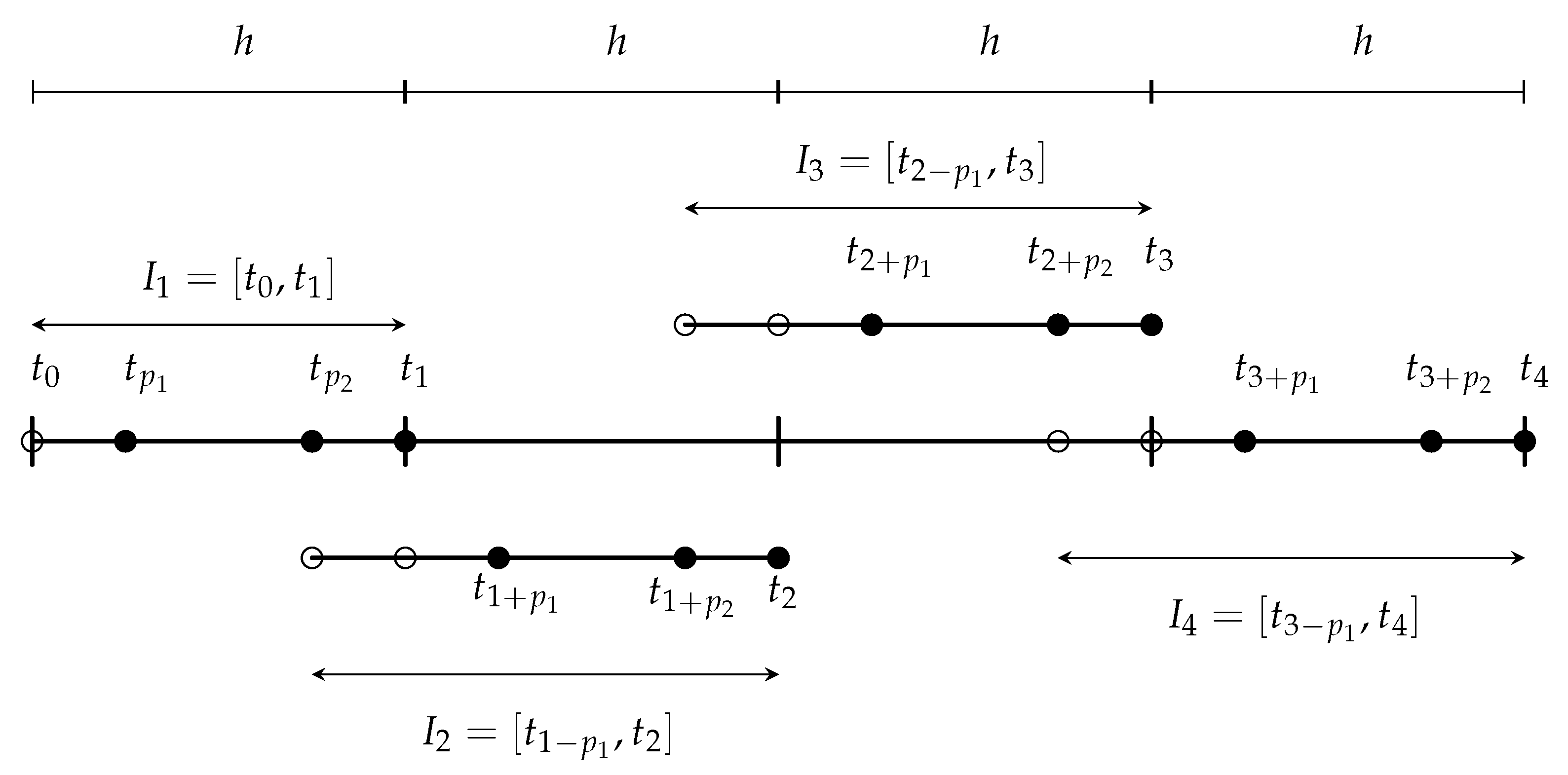
Let h be a prescribed step size on a mesh I defined by

$$I=\{t_n:t_0<t_1<\dots <t_N=T\}.$$

We choose $m+1$ collocation points, defined by

$$t_{n+p_i}=t_0+h{p}_i,i=0,1,2,\dots ,m$$

in the first interval $[t_0,t_1]$. For the intervals, $[t_n,t_{n+1}]$, where $1\le n\le N-1$, we choose $m+2$ collocation points:

$$\{t_{n-p_1}=t_n-h{p}_1\}\bigcup \left\{t_{n+p_i}=t_n+h{p}_i:i=0,1,2,\dots ,m\right\}.$$

The parameters $p_i$ are called collocation parameters, and they satisfy the condition

$$0=p_0<p_1<p_2<\cdots <p_{m-2}<p_{m-1}<p_m=1.$$

An illustrative representation of the grid is shown in Figure 1, for the special case when $m=3$ and $N=4$. It is worth noting that, for $n>0$, the grid $I_n$ overlaps with one grid point ($t_{n-1+p_{m-1}}=t_{n-p_1}$) from the previous grid $I_{n-1}$. For this reason, the method will be referred to as the overlapping hybrid block method.

In the non-overlapping block $I_1$, we suppose that the solution can be approximated by the polynomial:

$$y(t_0+sh),0\le s\le 1,$$

(2)

that satisfies the collocation conditions:

$$y^{\prime }\left(t_{p_i}\right)=f_{p_i}.$$

(3)

By the Lagrange interpolation formula, the function $y^{\prime }(t_0+sh)$ can be approximated as

$$y^{\prime }(t_0+sh)=\sum _{j=0}^m{y}^{\prime }\left(t_{p_j}\right){\ell }_j\left(s\right)$$

(4)

where

$${\displaystyle {\ell }_j\left(s\right)=\prod _{i=0,i\ne j}^m\frac{s-p_i}{p_j-p_i}.}$$

Using the collocation Equation (3), we obtain

$$y^{\prime }(t_0+sh)=\sum _{j=0}^m{f}_{p_j}{\ell }_j\left(s\right)$$

(5)

which is integrated from 0 to $p_i$ to give

$$y_{p_i}=y_0+h\sum _{j=0}^m{\beta }_{i,j}{f}_{p_j}$$

(6)

where

$${\beta }_{i,j}={\int }_0^{p_i}{\ell }_j\left(\tau \right)d\tau ,j=0,1,\dots ,m.$$

The matrix form of (6) is

$$A_1{Y}_1=A_0{Y}_0+h(B_0{F}_0+B_1{F}_1)$$

(7)

where

$$A_1=\left[\begin{array}{ccccc}1& 0& 0& \cdots & 0\\ 0& 1& 0& \cdots & 0\\ 0& 0& 1& \cdots & 0\\ ⋮& ⋮& ⋮& \ddots \\ 0& 0& 0& \cdots & 1\end{array}\right],A_0=\left[\begin{array}{ccccc}1& 0& 0& \cdots & 0\\ 1& 0& 0& \cdots & 0\\ 1& 0& 0& \cdots & 0\\ ⋮& ⋮& ⋮& \ddots \\ 1& 0& 0& \cdots & 0\end{array}\right]$$

$$B_0=\left[\begin{array}{ccccc}{\beta }_{1,0}& 0& 0& \cdots & 0\\ {\beta }_{2,0}& 0& 0& \cdots & 0\\ {\beta }_{3,0}& 0& 0& \cdots & 0\\ ⋮& ⋮& ⋮& \ddots \\ {\beta }_{m,0}& 0& 0& \cdots & 0\end{array}\right],B_1=\left[\begin{array}{ccccc}{\beta }_{1,1}& {\beta }_{1,2}& {\beta }_{1,3}& \cdots & {\beta }_{1,m}\\ {\beta }_{2,1}& {\beta }_{2,2}& {\beta }_{2,3}& \cdots & {\beta }_{2,m}\\ {\beta }_{3,1}& {\beta }_{3,2}& {\beta }_{3,3}& \cdots & {\beta }_{3,m}\\ ⋮& ⋮& ⋮& \ddots \\ {\beta }_{m,1}& {\beta }_{m,2}& {\beta }_{m,3}& \cdots & {\beta }_{m,m}\end{array}\right]$$

and

$$\begin{array}{cc}\hfill F_0& =\left[f_0,f_{-p_1},\dots ,f_{-p_{m-1}}\right],F_1=\left[f_{p_1},f_{p_2},\dots ,f_{p_m}\right],\hfill \\ \hfill Y_0& =\left[y_0,y_{-p_1},\dots ,y_{-p_{m-1}}\right],Y_1=\left[y_{p_1},y_{p_2},\dots ,y_{p_m}\right].\hfill \end{array}$$

In the block $I_n=[t_n,t_{n+1}]$ ($n>0$), we consider the collocation parameters

$$-p_1<0<p_1<p_2<\cdots <p_{m-1}<p_m$$

and assume the following collocation conditions:

$$y^{\prime }\left(t_{n+p_i}\right)=f_{n+p_i},y^{\prime }\left(t_{n-p_1}\right)=f_{n-p_1}$$

(8)

for $i=0,1,\dots ,m$. By the Lagrange interpolation formula, the function $y^{\prime }(t_n+sh)$ can be approximated as

$$y^{\prime }(t_n+sh)=\sum _{j=-1}^m{y}^{\prime }\left(t_{n+p_j}\right){\ell }_j\left(s\right).$$

(9)

Integrating from 0 to $p_i$ gives

$$y_{n+p_i}=y_n+h\sum _{j=-1}^m{\widehat{\beta }}_{i,j}{f}_{n+p_j}$$

(10)

where

$${\widehat{\beta }}_{i,j}={\int }_0^{p_i}{\ell }_j\left(\tau \right)d\tau ,j=-1,0,1,\dots ,m.$$

Equation (10) can be written in matrix form as

$$A_1{Y}_{n+1}=A_0{Y}_n+h({\widehat{B}}_0{F}_n+{\widehat{B}}_1{F}_{n+1})$$

(11)

where

$$Y_{n+1}=\left[\begin{array}{c}{y}_{n+p_1}\\ y_{n+p_2}\\ ⋮\\ y_{n+p_m}\end{array}\right],Y_n=\left[\begin{array}{c}{y}_n\\ y_{n-p_1}\\ ⋮\\ y_{n-p_{m-1}}\end{array}\right],F_{n+1}=\left[\begin{array}{c}{f}_{n+p_1}\\ f_{n+p_2}\\ ⋮\\ f_{n+p_m}\end{array}\right],F_n=\left[\begin{array}{c}{f}_n\\ f_{n-p_1}\\ ⋮\\ f_{n-p_{m-1}}\end{array}\right]$$

$${\widehat{B}}_0=\left[\begin{array}{cccc}{\widehat{\beta }}_{1,0}& {\widehat{\beta }}_{1,-1}& \cdots & 0\\ {\widehat{\beta }}_{2,0}& {\widehat{\beta }}_{2,-1}& \cdots & 0\\ ⋮& ⋮& \ddots & ⋮\\ {\widehat{\beta }}_{m,0}& {\widehat{\beta }}_{m,-1}& \cdots & 0\end{array}\right]{\widehat{B}}_1=\left[\begin{array}{cccc}{\widehat{\beta }}_{1,1}& {\widehat{\beta }}_{1,2}& \cdots & {\widehat{\beta }}_{1,m}\\ {\widehat{\beta }}_{2,1}& {\widehat{\beta }}_{2,2}& \cdots & {\widehat{\beta }}_{2,m}\\ ⋮& ⋮& \ddots & ⋮\\ {\widehat{\beta }}_{m,1}& {\widehat{\beta }}_{m,2}& \cdots & {\widehat{\beta }}_{m,m}\end{array}\right]$$

3. Analysis of the Method

In this section, we present the truncation error and stability properties of the proposed overlapping hybrid block method.

3.1. Local Truncation Error

Theorem 1. 

The local truncation error, in the integration block $[t_n,t_{n+1}]$, for the hybrid block method defined as

$$y_{n+p_i}=y_n+h\sum _{j=0}^m{\beta }_{i,j}{f}_{n+p_j},{\beta }_{i,j}={\int }_0^{p_i}{\ell }_j\left(\tau \right)d\tau$$

(12)

is given by

$$\begin{array}{cc}\hfill {\mathcal{L}}_i[z\left(t_n\right);h]& =\frac{h^{m+2}}{(m+2)!}\left[p_i^{m+2}-(m+2)\sum _{j=0}^m{\beta }_{i,j}{p}_j^{m+1}\right]z^{(m+2)}\left(t_n\right)+\mathcal{O}\left(h^{m+3}\right)\hfill \end{array}$$

(13)

for $i=1,2,\dots ,m$, when considering the grid points:

$$t_n<t_{n+p_1}<t_{n+p_1}<\cdots <t_{n+p_m}.$$

Proof. 

Given a sufficiently differentiable function $z\left(t\right)$, the truncation error of the hybrid block method can be written in terms of a linear operator ${\mathcal{L}}_i$ as

$${\mathcal{L}}_i[z\left(t_n\right);h]=z(t_n+h{p}_i)-z\left(t_n\right)-h\sum _{j=0}^m{\beta }_{i,j}{z}^{\prime }(t_n+h{p}_j),i=1,2,\dots ,m.$$

(14)

Using Taylor series to expand (14) gives

$$\begin{array}{cc}\hfill {\mathcal{L}}_i[z\left(t_n\right);h]& =\sum _{k=1}^K\frac{p_i^k}{k!}{h}^k{z}^{\left(k\right)}\left(t_n\right)-\sum _{k=1}^K\frac{h^{k}k}{k!}\sum _{j=0}^m{\beta }_{i,j}{p}_j^{k-1}{z}^{\left(k\right)}\left(t_n\right)+O\left(h^{K+1}\right)\hfill \\ \hfill & =\sum _{k=2}^{m+1}\frac{h^k}{k!}\left[p_i^k-k\sum _{j=0}^m{\beta }_{i,j}{p}_j^{k-1}\right]z^{\left(k\right)}\left(t_n\right)\hfill \\ \hfill & +\sum _{k=m+2}^K\frac{h^k}{k!}\left[p_i^k-k\sum _{j=0}^m{\beta }_{i,j}{p}_j^{k-1}\right]z^{\left(k\right)}\left(t_n\right)+\mathcal{O}\left(h^{K+1}\right)\hfill \end{array}$$

(15)

where $K\ge m+2$ is a positive integer.

Using the identity:

$${\displaystyle \sum _{j=0}^m{\ell }_j\left(x\right)=1}$$

we note that

$$\sum _{j=0}^m{\beta }_{i,j}=\sum _{j=0}^m{\int }_0^{p_i}{\ell }_j\left(x\right)dx=p_i$$

and

$$\sum _{j=0}^m{\beta }_{i,j}{p}_j^{k-1}=\sum _{j=0}^m\left({\int }_0^{p_i}{\ell }_j\left(x\right)dx\right)p_j^{k-1}=\frac{p_i^k}{k},fork=2,\dots ,m+1.$$

(16)

In a related study on implicit Runge–Kutta processes, the identity (16) was also reported by [10]. Substituting the identities in (15) gives the result in (13). □

As an immediate consequence, we obtain the following result, for the truncation error in the integration blocks $[t_n,t_{n+1}]$ ($n>0$):

Corollary 1. 

The local truncation error, in the integration block $[t_n,t_{n+1}]$, for the one-point overlapping hybrid block method:

$$y_{n+p_i}=y_n+h\sum _{j=-1}^m{\widehat{\beta }}_{i,j}{f}_{n+p_j},{\widehat{\beta }}_{i,j}={\int }_0^{p_i}{\ell }_j\left(\tau \right)d\tau$$

(17)

is

$$\begin{array}{cc}\hfill {\mathcal{L}}_i[z\left(t_n\right);h]& =\frac{h^{m+3}}{(m+3)!}\left[p_i^{m+3}-(m+3)\sum _{j=0}^{m+1}{\widehat{\beta }}_{i,j-1}{p}_{j-1}^{m+2}\right]z^{(m+3)}\left(t_n\right)+\mathcal{O}\left(h^{m+4}\right).\hfill \end{array}$$

(18)

Proof. 

The proof is similar to the one for Theorem 1, given above, and uses the identity:

$$\sum _{j=0}^{m+1}{\widehat{\beta }}_{i,j-1}{p}_{j-1}^{k-1}=\sum _{j=0}^{m+1}\left({\int }_0^{p_i}{\ell }_{j-1}\left(x\right)dx\right)p_{j-1}^{k-1}=\frac{p_i^k}{k},for k=2,\dots ,m+2$$

after considering the $m+2$ grid points:

$$t_{n-p_1}<t_n<t_{n+p_1}<t_{n+p_1}<\cdots <t_{n+p_m}.$$

□

By minimizing the local truncation error of the main method at $t_{n+1}$ (i.e., $p_m=1$), it was shown in [11] that the optimal intra-step points are the roots of the polynomial:

$$Q_i\left(p\right)=\frac{1}{i(i+1)}\sum _{k=1}^i\frac{k{(-1)}^{i+k}{p}^{k-1}(i+k)!}{{(k!)}^2(i-k)!}$$

(19)

which is proportional to the first derivative of the shifted Legendre polynomials of degree m given by

$$P_i^{*}\left(t\right)=\sum _{k=0}^i\frac{{(-1)}^{i+k}{t}^k(i+k)!}{{(k!)}^2(i-k)!}.$$

(20)

The shifted Legendre polynomials are defined in $[0,1]$ and have the property:

$$P_i^{*}(1-t)={(-1)}^i{P}_i^{*}\left(t\right),i=0,1,2,\dots .$$

(21)

Furthermore, $P_i^{*}\left(t\right)$ has i distinct roots in $(0,1)$. By expanding (19), we obtain the polynomials that give optimal intra-step points with $m=2,3,4,5$ as follows:

$$\begin{array}{cc}\hfill Q_2\left(p\right)& =2p-1,\hfill \\ \hfill Q_3\left(p\right)& =5p^2-5p+1,\hfill \\ \hfill Q_4\left(p\right)& =14p^3-21p^2+9p-1,\hfill \\ \hfill Q_5\left(p\right)& =42p^4-84p^3+56p^2-14p+1,\hfill \\ \hfill Q_6\left(p\right)& =132p^5-330p^4+300p^3-120p^2+20p-1.\hfill \end{array}$$

As a consequence of Equation (21), the optimal roots (intra-step points) have the form

$$\left\{p_1,p_2,\dots ,\dots ,p_{\frac{m}{2}-\frac{1}{2}},1-p_{\frac{m}{2}-\frac{1}{2}},\dots ,1-p_2,1-p_1\right\}$$

when m is odd and

$$\left\{p_1,p_2,\dots ,\dots ,p_{\frac{m}{2}-1},\frac{1}{2},1-p_{\frac{m}{2}-1},\dots ,1-p_2,1-p_1\right\}$$

when m is even.

The truncation errors for overlapping and non-overlapping HBM algorithms with equally spaced and optimally spaced intra-step points are compared in

Table 1. Truncation errors for the overlapping and non-overlapping HBM with equally spaced and optimal intra-step points.

		Equally Spaced		Optimal Points
	${\mathcal{L}}_i$	Non-Overlapping	Overlapping	Non-Overlapping	Overlapping
	$p_1$	$-\frac{19y^{\left(5\right)}\left(t_n\right)h^5}{174960}$	$-\frac{11y^{\left(6\right)}\left(t_n\right)h^6}{1049760}$	$-\frac{y^{\left(5\right)}\left(t_n\right)h^5}{6000\sqrt{5}}$	$\frac{\left(4-3\sqrt{5}\right)y^{\left(6\right)}\left(t_n\right)h^6}{450000}$
$m=3$	$p_2$	$-\frac{y^{\left(5\right)}\left(t_n\right)h^5}{21870}$	$\frac{y^{\left(7\right)}\left(t_n\right)h^7}{1653372}$	$\frac{y^{\left(5\right)}\left(t_n\right)h^5}{6000\sqrt{5}}$	$\frac{\left(1+3\sqrt{5}\right)y^{\left(6\right)}\left(t_n\right)h^6}{450000}$
	$p_3$	$-\frac{y^{\left(5\right)}\left(t_n\right)h^5}{6480}$	$-\frac{y^{\left(6\right)}\left(t_n\right)h^6}{38880}$	$-\frac{y^{\left(7\right)}\left(t_n\right)h^7}{1512000}$	$-\frac{y^{\left(7\right)}\left(t_n\right)h^7}{1512000}$
	$p_1$	$\frac{3y^{\left(6\right)}\left(t_n\right)h^6}{655360}$	$\frac{271y^{\left(7\right)}\left(t_n\right)h^7}{990904320}$	$\frac{y^{\left(6\right)}\left(t_n\right)h^6}{493920}$	$\frac{\left(49-8\sqrt{21}\right)y^{\left(7\right)}\left(t_n\right)h^7}{145212480}$
$m=4$	$p_2$	$\frac{y^{\left(6\right)}\left(t_n\right)h^6}{368640}$	$\frac{y^{\left(7\right)}\left(t_n\right)h^7}{12386304}$	$-\frac{y^{\left(6\right)}\left(t_n\right)h^6}{322560}$	$\frac{\left(-14+\sqrt{21}\right)y^{\left(7\right)}\left(t_n\right)h^7}{27095040}$
	$p_3$	$\frac{3y^{\left(6\right)}\left(t_n\right)h^6}{655360}$	$\frac{13y^{\left(7\right)}\left(t_n\right)h^7}{36700160}$	$\frac{y^{\left(6\right)}\left(t_n\right)h^6}{493920}$	$\frac{\left(49+\sqrt{21}\right)y^{\left(7\right)}\left(t_n\right)h^7}{145212480}$
	$p_4$	$-\frac{y^{\left(7\right)}\left(t_n\right)h^7}{1935360}$	$-\frac{y^{\left(7\right)}\left(t_n\right)h^7}{1935360}$	$-\frac{y^{\left(9\right)}\left(t_n\right)h^9}{1422489600}$	$-\frac{y^{\left(9\right)}\left(t_n\right)h^9}{1422489600}$
	$p_1$	$-\frac{863y^{\left(7\right)}\left(t_n\right)h^7}{4725000000}$	$-\frac{13y^{\left(8\right)}\left(t_n\right)h^8}{1750000000}$	$-\frac{\left(\sqrt{147-30\sqrt{7}}{y}^{\left(7\right)}\left(t_n\right)\right)h^7}{160030080}$	$\frac{\left(-12\sqrt{147-30\sqrt{7}}+26\sqrt{7}+13\right)y^{\left(8\right)}\left(t_n\right)h^8}{13442526720}$
	$p_2$	$-\frac{37y^{\left(7\right)}\left(t_n\right)h^7}{295312500}$	$-\frac{y^{\left(8\right)}\left(t_n\right)h^8}{295312500}$	$\frac{\sqrt{147+30\sqrt{7}}{y}^{\left(7\right)}\left(t_n\right)h^7}{160030080}$	$6.05861\times {10}^{-9}{y}^{\left(8\right)}\left(t_n\right)h^8$
$m=5$	$p_3$	$-\frac{29y^{\left(7\right)}\left(t_n\right)h^7}{175000000}$	$-\frac{13y^{\left(8\right)}\left(t_n\right)h^8}{1750000000}$	$-\frac{\left(\sqrt{147+30\sqrt{7}}{y}^{\left(7\right)}\left(t_n\right)\right)h^7}{160030080}$	$-1.05281\times {10}^{-8}{y}^{\left(8\right))}{h}^8$
	$p_4$	$-\frac{8y^{\left(7\right)}\left(t_n\right)h^7}{73828125}$	$\frac{13y^{\left(9\right)}\left(t_n\right)h^9}{27685546875}$	$\frac{\sqrt{147-30\sqrt{7}}{y}^{\left(7\right)}\left(t_n\right)h^7}{160030080}$	$\frac{\left(12\sqrt{147-30\sqrt{7}}+2\sqrt{7}+1\right)y^{\left(8\right)}\left(t_n\right)h^8}{13442526720}$
	$p_5$	$-\frac{11y^{\left(7\right)}\left(t_n\right)h^7}{37800000}$	$-\frac{11y^{\left(8\right)}\left(t_n\right)h^8}{378000000}$	$-\frac{y^{\left(11\right)}{h}^{11}}{2112397056000}$	$-\frac{y^{\left(11\right)}\left(t_n\right)h^{11}}{2112397056000}$

for $m=3,4,5$. The table reveals that the truncation errors of the overlapping HBM are at least h orders of magnitude smaller than those of the non-overlapping HBM. This is consistent with the observations made in the preceding theorems regarding the explicit formulas for local truncation errors.

3.2. Zero Stability

In the limit when $h\to 0$, the zero stability of the hybrid methods for all blocks ($n=0,1,\dots ,N-1$) can be analysed from the zeros of the polynomial that is computed from

$$\rho \left(\lambda \right)=det\left[A_1\lambda -A_0\right].$$

(22)

Zero stability is confirmed if the roots of $\rho \left(\lambda \right)$ satisfy $|{\lambda }_j|\le 1$ and all the roots with

$|{\lambda }_j|=1$ have a multiplicity of 1. The characteristic polynomial for the hybrid block methods considered in this study is

$$\rho \left(\lambda \right)={\lambda }^m(\lambda -1).$$

Thus, the proposed overlapping hybrid block methods are zero stable for any selection of intra-step points. In a related investigation, Reference [1] also validated the zero stability of the HBMs.

3.3. Absolute Stability

If errors introduced in one time step do not accumulate in successive time steps, the general stability of a numerical approach is confirmed. A region of absolute stability is defined as the set of points $z\in \mathbb{C}$ such that the roots of the characteristic equation associated with the test equation $y^{\prime }=\lambda y$ ($\lambda <0$) lie within a unit circle. For hybrid block methods, the absolute stability in the first non-overlapping interval is well established (see, for example, [5]). When this test problem is applied to the overlapping grid methods (11), the following matrix equation is obtained:

$$Y_{n+1}=R\left(z\right)Y_n$$

(23)

where $z=\lambda h$ and $R\left(z\right)$ is a matrix equation given by

$$R\left(z\right)={(A_1-z{\widehat{B}}_1)}^{-1}(A_0+z{\widehat{B}}_0).$$

(24)

By finding the eigenvalues of the matrix $R\left(z\right),$ one can derive the stability function $H\left(z\right)$. Figure 2 depicts, for illustrative purposes, the absolute stability region of the proposed overlapping grid hybrid block method created from optimally spaced and equally spaced intra-step points for $m=3$. Given that the shaded area encompasses the entirety of the left half-plane, the absolute stability of the overlapping HBM is confirmed for both equally spaced and optimal intra-step points.

4. Numerical Experimentation and Results

In this section, we implement the proposed overlapping hybrid block method to generate numerical solutions for problems that are typically difficult to solve numerically using standard methods. Before employing the hybrid block approach to integrate the nonlinear IVPs, they are first linearized. For a general nonlinear system of first-order IVPs, the linearisation method is detailed below.

Consider the system of s nonlinear first-order IVPs of the form

$$\begin{array}{cc}\hfill y_k^{\prime }=f_k(t,y_1,\dots ,y_s)& ={\mathcal{L}}_k(t,y_1,\dots ,y_{k-1},y_{k+1},\dots ,y_s)y_k\hfill \\ \hfill & +{\mathcal{N}}_k(t,y_1,\dots ,y_{k-1},y_k,y_{k+1}\dots ,y_s)\hfill \end{array}$$

(25)

where ${\mathcal{L}}_k(\cdots )$ is the coefficient of the state variable $y_k$, and ${\mathcal{N}}_k(\cdots )$ is the component of the k-th equation that is not linear in $y_k$, for $k=1,2,\dots ,s$. The hybrid block method is sequentially applied iteratively to each equation in the system (25), with the solution of the k-th equation used immediately when solving the $(k+1)$th equation. Consequently, the iterative scheme is developed as

$$\begin{array}{cc}\hfill y_{k,r+1}^{\prime }& ={\mathcal{L}}_k(t,y_{1,r+1},\dots ,y_{k-1,r+1},y_{k+1,r},\dots ,y_{s,r})y_{k,r+1}\hfill \\ \hfill & +{\mathcal{N}}_k(t,y_{1,r+1},\dots ,y_{k-1,r+1},y_{k,r},\dots ,y_{s,r}).\hfill \end{array}$$

(26)

This linearization method employs the Gauss–Seidel method for decoupling and solving large systems of nonlinear equations. The method has been adapted from the waveform relaxation method that has been reported in the literature (see, for example, [12,13]).

Noting that (26) is linear, it can be applied to the HBM method after setting

$$f(t,y)=\varphi \left(t\right)y+\psi \left(t\right)$$

where $\varphi =\mathcal{L}(\cdots )$ and $\psi =\mathcal{N}(\cdots )$ are known functions of t. As a result, the matrix form of the HBM, (11), becomes

$$A_1{Y}_{n+1}=A_0{Y}_n+h{\widehat{B}}_0({\mathit{\varphi }}_{\mathit{n}}^{\left(d\right)}{Y}_n+{\mathit{\psi }}_n)+h{\widehat{B}}_1({\mathit{\varphi }}_{\mathit{n}+\mathbf{1}}^{\left(d\right)}{Y}_{n+1}+{\mathit{\psi }}_{n+1})$$

(27)

or

$$P_n{Y}_{n+1}=Q_n$$

(28)

where

$$\begin{array}{cc}\hfill P_n& =A_1-h{\widehat{B}}_1{\mathit{\varphi }}_{\mathit{n}+\mathbf{1}}^{\left(d\right)},\hfill \\ \hfill Q_n& =\left(A_0+h{\widehat{B}}_0{\mathit{\varphi }}_{\mathit{n}}^{\left(d\right)}\right)Y_n+h\left({\widehat{B}}_0{\mathit{\psi }}_n+{\widehat{B}}_1{\mathit{\psi }}_{n+1}\right)\hfill \end{array}$$

$$\begin{array}{cc}\hfill {\mathit{\psi }}_n& ={\left[{\psi }_n,{\psi }_{n-p_1},\dots ,{\psi }_{n-p_{m-1}}\right]}^T,{\mathit{\psi }}_{n+1}={\left[{\psi }_{n+p_1},{\psi }_{n+p_2},\dots ,{\psi }_{n+p_m}\right]}^T,\hfill \end{array}$$

$${\mathit{\varphi }}_n^{\left(d\right)}=\left[\begin{array}{cccc}{\varphi }_n& & & \\ & {\varphi }_{n-p_1}& & \\ & & & \\ & & & {\varphi }_{n-p_{m-1}}\end{array}\right],{\mathit{\varphi }}_{n+1}^{\left(d\right)}=\left[\begin{array}{cccc}{\varphi }_{n+p_1}& & & \\ & {\varphi }_{n+p_2}& & \\ & & & \\ & & & {\varphi }_{n+p_m}\end{array}\right]$$

All numerical examples in this study were solved using (28) applied iteratively over 20 iterations for each integration block $[t_n,t_{n+1}]$. Through numerical experimentation, it was determined that sufficient convergence would have occurred prior to the 20th iteration level. All numerical results presented in this study were generated by iterating the scheme (28) up to $r=20$ for all n values. In light of the linearisation of nonlinear IVPs via partitioning, the hybrid block method defined by (28) is referred to as the linear partitioning overlapping hybrid block method. The method is computationally efficient and easy to implement. Due to the lack of derivatives and Jacobian matrices, it circumvents the challenges of Newton-based iterative techniques that rely on derivatives.

In the examples, given below, the linear partitioning overlapping hybrid block method was applied using equally spaced and the shifted Legendre-based optimal intra-step points. In both cases, $m=3$ and $m=5$ were used for illustrative purposes. The intra-step points corresponding to these values of m are given in

Table 2. Intra-step points used in numerical experimentation.

m	Equidistant	Optimal Points
3	${\displaystyle \frac{1}{3},\frac{2}{3}}$	${\displaystyle \frac{1}{10}(5\pm \sqrt{5})}$
5	${\displaystyle \frac{1}{5},\frac{2}{5},\frac{3}{5},\frac{4}{5}}$	${\displaystyle \frac{1}{2}\left(1\pm \sqrt{\frac{1}{21}\left(7\pm 2\sqrt{7}\right)}\right)}$

below.

Using $m=3$ as an example, the matrix parameters for the optimal overlapping hybrid block approach are as follows:

$$B_0=\left[\begin{array}{ccc}\frac{\sqrt{5}+11}{120}& 0& 0\\ \frac{11-\sqrt{5}}{120}& 0& 0\\ \frac{1}{12}& 0& 0\end{array}\right],B_1=\left[\begin{array}{ccc}\frac{25-\sqrt{5}}{120}& \frac{25-13\sqrt{5}}{120}& \frac{\sqrt{5}-1}{120}\\ \frac{13\sqrt{5}+25}{120}& \frac{\sqrt{5}+25}{120}& \frac{-\sqrt{5}-1}{120}\\ \frac{5}{12}& \frac{5}{12}& \frac{1}{12}\end{array}\right]$$

which is applied on the scheme:

$$A_1{Y}_1=A_0{Y}_0+h(B_0{F}_0+B_1{F}_1)$$

(29)

in the first interval $[t_0,t_1]$ and

$${\widehat{B}}_0=\left[\begin{array}{ccc}\frac{11\sqrt{5}+61}{600}& \frac{-5\sqrt{5}-9}{2200}& 0\\ \frac{49-11\sqrt{5}}{600}& \frac{5\sqrt{5}+9}{2200}& 0\\ \frac{1}{12}& 0& 0\end{array}\right],{\widehat{B}}_1=\left[\begin{array}{ccc}\frac{55-4\sqrt{5}}{300}& \frac{137-65\sqrt{5}}{600}& \frac{37\sqrt{5}-61}{6600}\\ \frac{17\sqrt{5}+35}{150}& \frac{5\sqrt{5}+113}{600}& \frac{-37\sqrt{5}-49}{6600}\\ \frac{5}{12}& \frac{5}{12}& \frac{1}{12}\end{array}\right]$$

which is applied in $[t_n,t_{n+1}]$, for the overlapping hybrid block scheme:

$$A_1{Y}_1=A_0{Y}_0+h({\widehat{B}}_0{F}_0+{\widehat{B}}_1{F}_1)$$

(30)

for $n=1,2,\dots ,N-1$. The proposed overlapping grid approach is referred to as the overlapping optimal hybrid block method (OOHBM) for the purposes of this paper. The original optimal hybrid block method (OHBM), without overlap, is constructed by applying Equation (29) to all the integration blocks $[t_n,t_{n+1}]$ for $n=0,1,2,\dots ,N-1$. It is important to note that the size of the matrices in both the original HBM scheme and the overlapping HBM scheme is the same. This indicates that the computational effort necessary to solve the IVPs will be roughly equivalent for both methods.

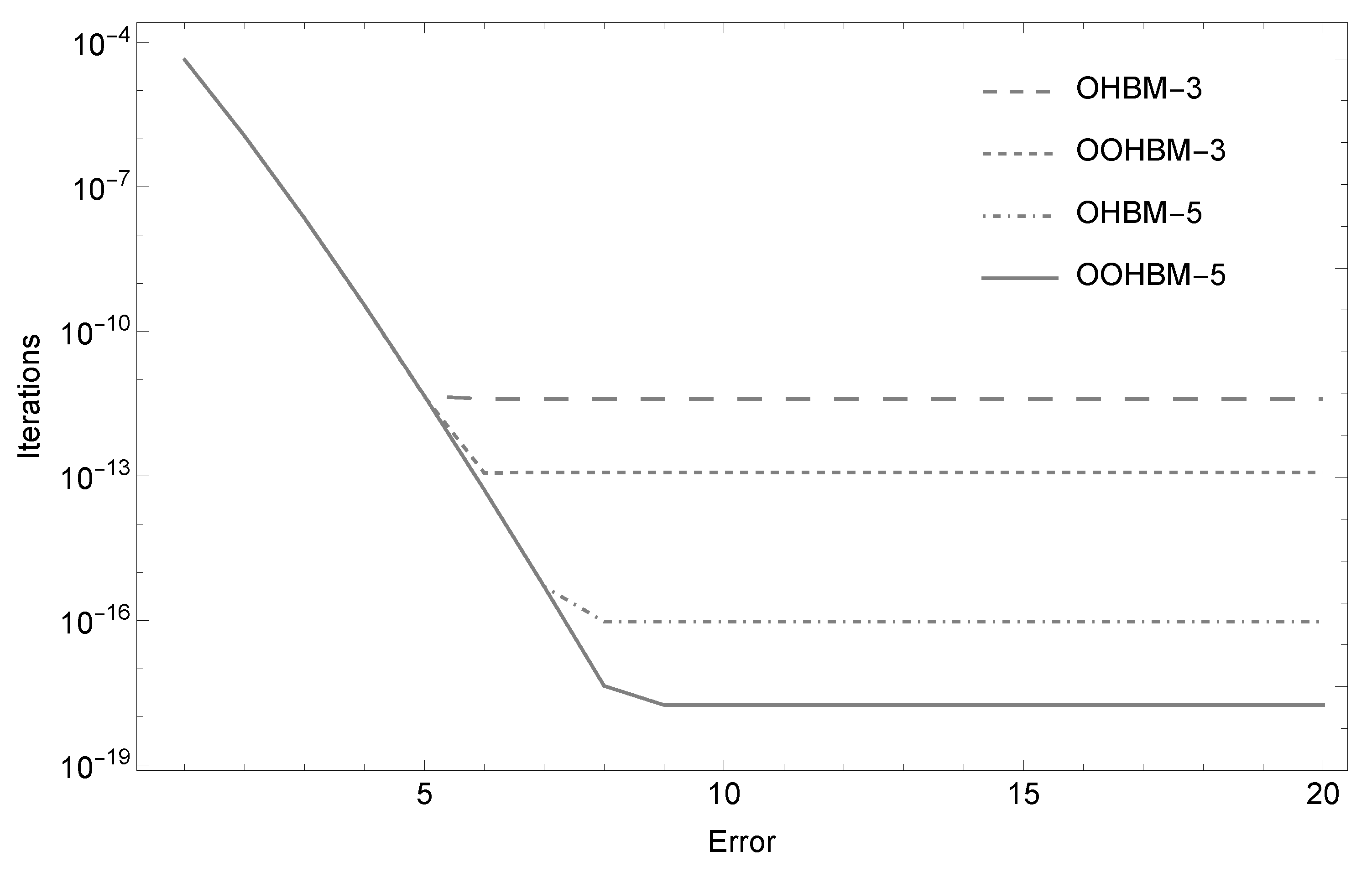
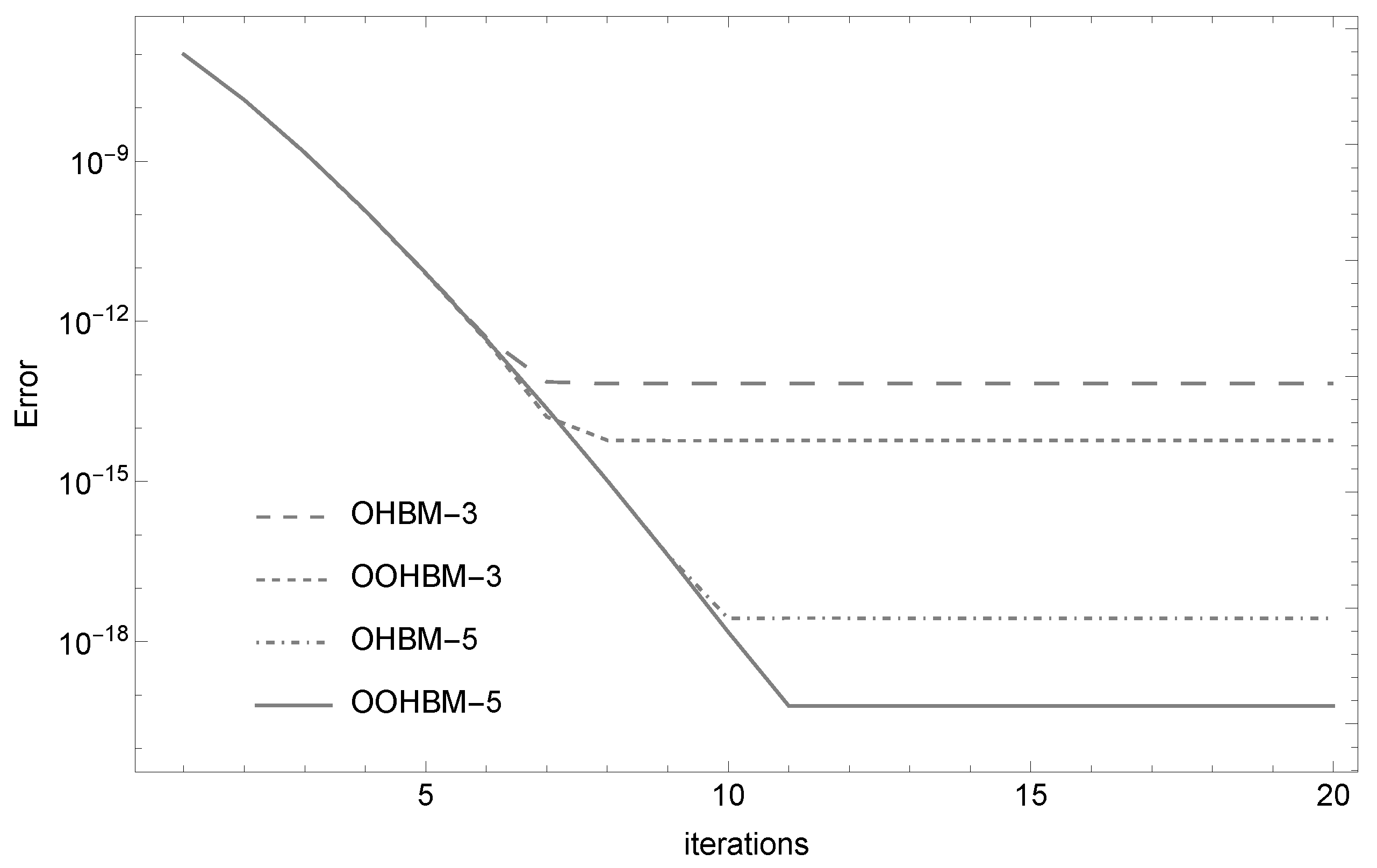
4.1. Example 1

Consider the following example that belongs to the class of problems with the so-called Runge phenomenon:

$$y^{\prime }=144(1-2t)y^2,y\left(0\right)=\frac{1}{37}.$$

(31)

The exact solution of Example (31) is ${\displaystyle y\left(t\right)=\frac{1}{36{(2t-1)}^2+1}}$. In this example, the linear partitioning iterative method with

$$\varphi (t,y_r)=144(1-2t)y_r^2,\psi (t,y_r)=0$$

was used with the HBM schemes to solve (31) using $h=0.01$ and up to 20 iterations, within the integration domain [0,1]. The convergence plot, computed as the maximum error per iteration in the last block $[t_{N-1},t_N]$, is shown in Figure 3. The convergence of the optimal overlapping (OOHBM) and the original optimal hybrid block technique (OHBM) with no overlapping grid for $m=3$ and $m=5$ are compared. The graph demonstrates that the overlapping HBM plateaus at a higher degree of accuracy than the non-overlapping HBM. This is one indicator of the overlapping HBM’s higher precision. It is also apparent from Figure 3 that the linear partitioning HBM converges swiftly, with full convergence reached within 10 iterations for all HBM variants evaluated in this scenario.

A comparison of the maximum absolute errors, computed from the exact solution, is displayed in

Table 3. Maximum errors for Example 1 using different choices of intra-step points.

	$\mathit{m}=3$		$\mathit{m}=5$
	Original HBM	Proposed HBM	Original HBM	Proposed HBM
Equally spaced points	$9.9970\times {10}^{-7}$	$6.7542\times {10}^{-8}$	$6.0825\times {10}^{-10}$	$4.2735\times {10}^{-11}$
Optimal points	$1.8106\times {10}^{-7}$	$3.2112\times {10}^{-8}$	$1.4701\times {10}^{-10}$	$1.5855\times {10}^{-11}$

. It can be seen from the table that the maximum error improves when the overlapping grid is applied. In this example, the improvement in the maximum error when comparing equally spaced and optimal hybrid block methods is not as significant as the difference between the original and proposed overlapping HBM. It can also be observed that the maximum error obtained using the overlapping HBM with equally spaced points is greater than the error of the original optimal HBM, for both $m=3$ and $m=5$. This appears to indicate that introducing grid overlap into HBM systems reduces the maximum error more than adjusting the type of intra-step points.

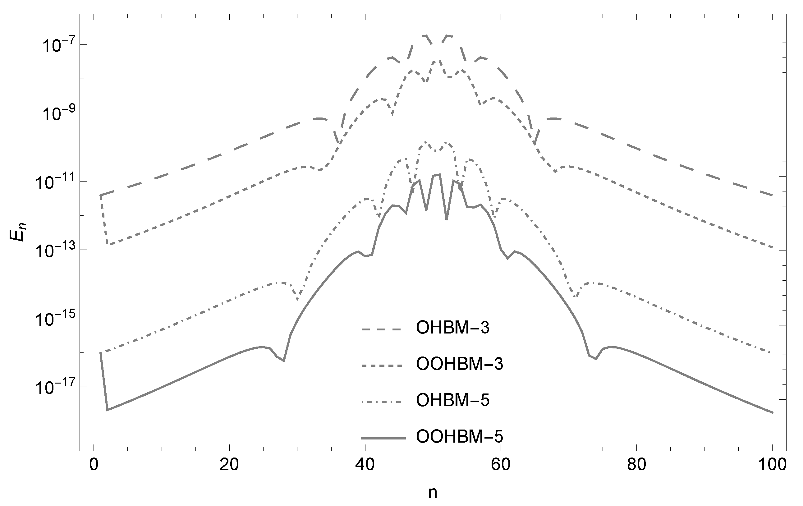
The maximum error in each block $[t_n,t_{n+1}]$ is defined as

$$E_n=\underset{1\le i\le m}{\max }|y\left(x_{n+p_i}\right)-y_{n+p_i}|.$$

(32)

Plotting the profile of the maximum error in each block for $n=0,1,\dots ,N-1$ reveals the distribution of the error as it traverses the complete domain of integration. Figure 4 depicts the maximum error profile $E_n$ for 100 intervals (blocks) used during the deployment of the overlapping optimal HBM and original optimal HBM to Example 31. The graph illustrates the significant reduction in the maximum error when the overlapping grid method is implemented. The maximum error begins in the same location when $n=0$. This is expected given that the initial interval is identical for both optimal overlapping (OOHBMs) and standard optimal non-overlapping HBMs (OHBMs). After $n=0$, the maximum errors of the OOHBM are less than those of the OHBM when $m=3$ and when $m=5$. The reduction in the computed error is consistent with the theorems for local truncation errors derived in the preceding section, which demonstrates that the truncation error of the overlapping HBM is $O\left(h\right)$ more than that of the corresponding non-overlapping HBM.

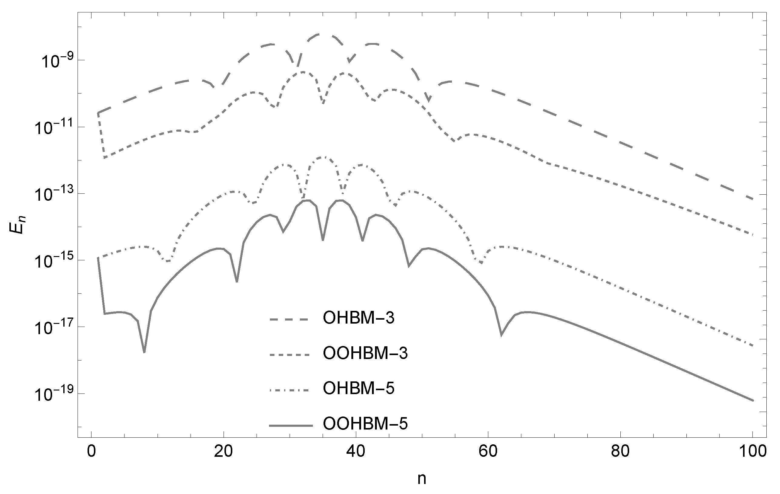
4.2. Example 2

Consider the logistic equation:

$$y^{\prime }=\kappa y(1-y),y\left(0\right)=y_0$$

(33)

with the exact solution ${\displaystyle y\left(t\right)=\frac{y_0}{(1-y_0)e^{-\kappa t}+y_0}}$. The problem was integrated on $[0,10]$ using a step size of $h=0.1$ for the case when $\kappa =2$.

Table 4. Maximum errors for Example 2 using different choices of intra-step points.

	$\mathit{m}=3$		$\mathit{m}=5$
	Original HBM	Proposed HBM	Original HBM	Proposed HBM
Equally spaced points	$1.3918\times {10}^{-7}$	$1.5292\times {10}^{-8}$	$7.2577\times {10}^{-12}$	$8.5256\times {10}^{-13}$
Optimal points	$6.3022\times {10}^{-9}$	$4.4041\times {10}^{-10}$	$1.2751\times {10}^{-12}$	$6.2343\times {10}^{-14}$

compares the maximum errors produced by the OOHBM versus the OHBM. Included also are the maximum errors of the corresponding hybrid block methods constructed using intra-step points equally spaced apart. The table clearly illustrates the increase in accuracy brought about by the introduction of overlapping in grids that use both equally spaced and optimal intra-step points.

Figure 5 provides a comparison of the convergence plots for the standard OHBM and the proposed OOHBM. The illustration demonstrates the speedy convergence of the linear partitioning iterative approach and the superior accuracy of the proposed OOHBM schemes in comparison to the OHBM schemes.

Figure 6 illustrates the maximum error profile $E_n$ across all blocks as a function of the block index n. The decrease in error shown in Figure 6 when switching from the OHBM to the OOHBM is consistent with the pattern observed in Figure 4 of the preceding case. This is additional proof that the concept of overlapping grids improves the accuracy of hybrid methods.

Next, we discuss the implementation of the overlapping HBM on systems of nonlinear equations that are notoriously difficult to numerically solve due to their stiff characteristics or their propensity to change rapidly over short time intervals.

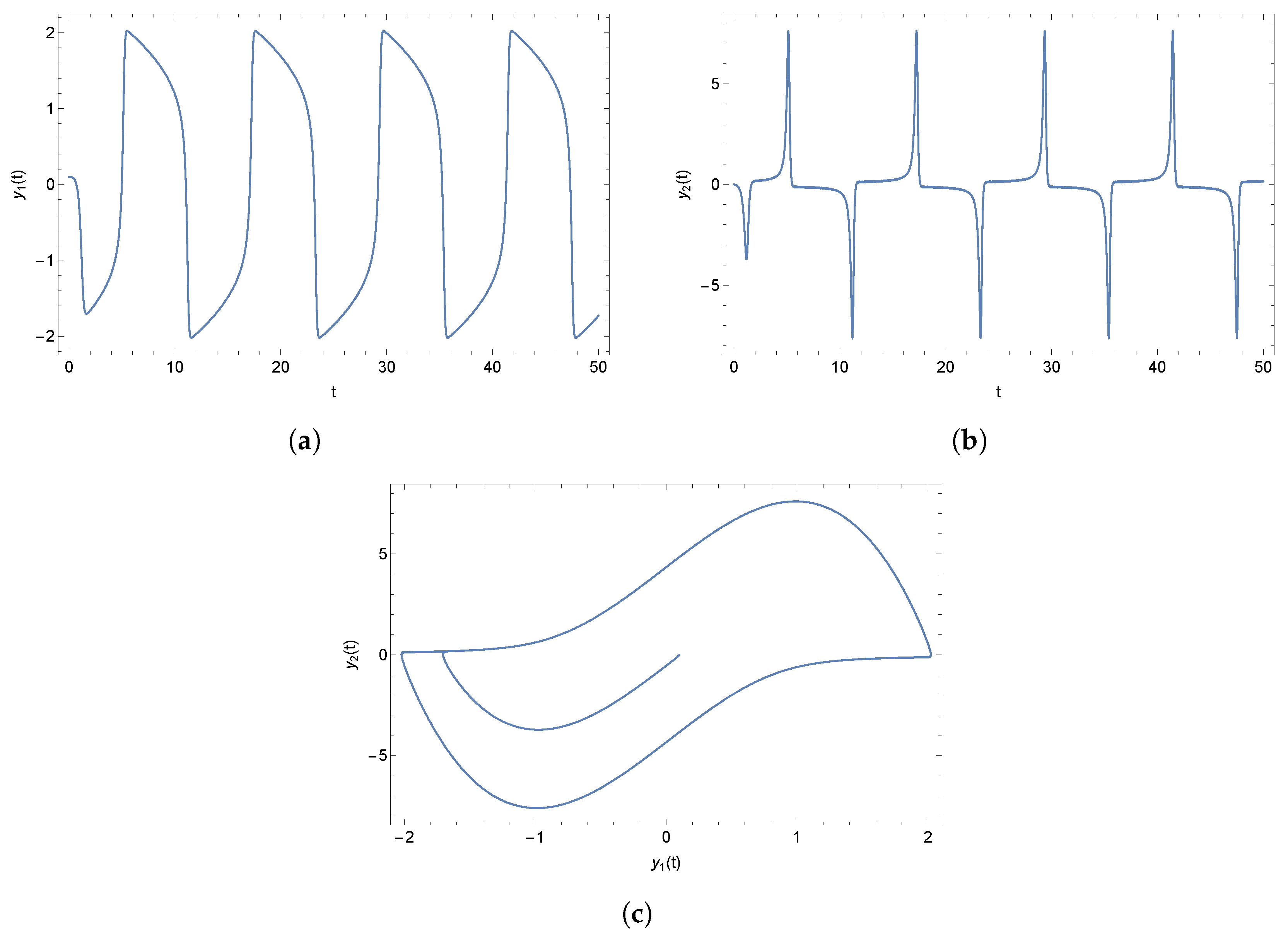
4.3. Example 3

Consider the the van der Pol oscillator with nonlinear damping:

$$\begin{array}{cc}\hfill y_1^{\prime }& =y_2,y_1\left(0\right)=0.1,\hfill \\ \hfill y_2^{\prime }& =\mu (1-y_1^2)y_2-y_1,y_2\left(0\right)=0\hfill \end{array}$$

where $\mu$ is a constant parameter. In this example, we set

$${\psi }_1(t,y_r,{\dot{y}}_r)=y_{2,r},{\varphi }_1(t,y_r,{\dot{y}}_r)=0,{\psi }_2(t,y_r,{\dot{y}}_r)=-y_{1,r+1},{\varphi }_2(t,y_r,{\dot{y}}_r)=\mu (1-y_{1,r+1}^2).$$

This problem was solved using the OOHBM-3 with $h=0.01$ in the domain of integration [0,50]. Since there is no analytic solution to the problem, we compared the results of the solution profiles to those that have been previously reported in the literature. In Figure 7, the solution profiles and phase portrait for the van der Pol oscillator when $\mu =5$ are depicted. Similar results have been reported in the literature using different numerical solution techniques (see, for example, [14]).

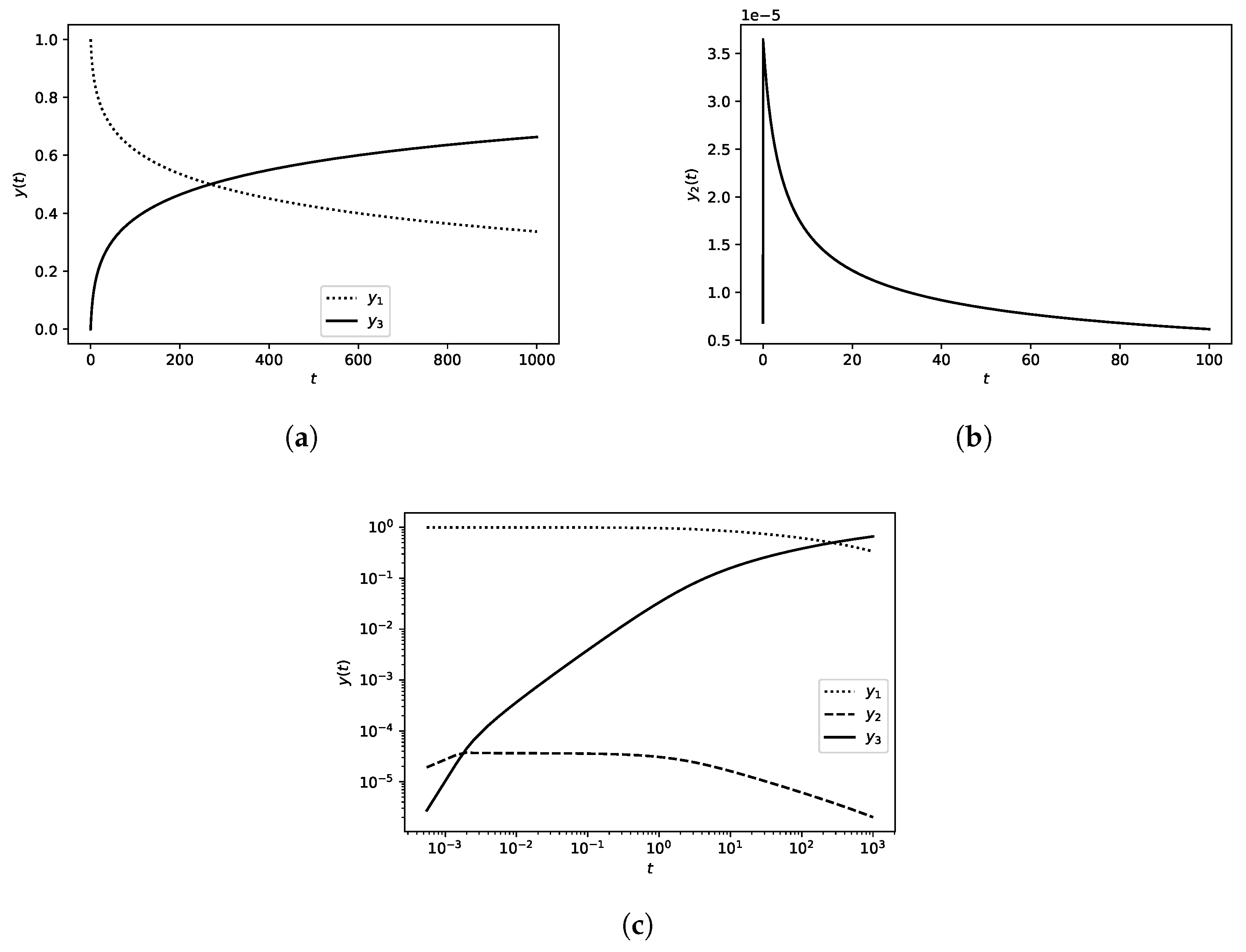
4.4. Example 4

Consider the highly stiff system of IVPs below, which has applications in chemical kinetics [15].

$$\begin{array}{cccc}{y}_1^{\prime }& =-k_1{y}_1+k_2{y}_2{y}_3,\hfill & y_1\left(0\right)\hfill & =1,\hfill \\ y_2^{\prime }& =k_1{y}_1-k_2{y}_2{y}_3-k_3{y}_2^2,\hfill & y_2\left(0\right)\hfill & =0,\hfill \\ y_3^{\prime }& =k_3{y}_2^2,\hfill & y_3\left(0\right)\hfill & =0,\hfill \end{array}$$

For specific values of the reaction constants, this problem becomes highly stiff and unsolvable using ordinary numerical approaches. In this study, we employed the values that were also used to assess the robustness of the extended backward difference methods described in [16] and the implicit Runge–Kutta method as summarized in [17]. Consequently, we set

$$k_1=0.04,k_2={10}^4,k_3=3\times {10}^7.$$

Figure 8 depicts the solution profiles generated by OOHBM-3 with $h=0.001$. The nature of the solution profile for $y_2$ provides insight into the numerical difficulties of solving this problem. Over a brief period of time, the concentration of $y_2$ rises abruptly to a maximum and then falls sharply. Compared to the concentrations of $y_1$ and $y_3$ represented in Figure 8a, the size of the concentration for $y_2$ is less. Due to the widely different concentration amounts, the $log$ plot on the x-axis is used to compare all the concentration profiles over a longer period of time, as depicted in Figure 8c. These profiles are comparable to those published in [17].

4.5. Example 5

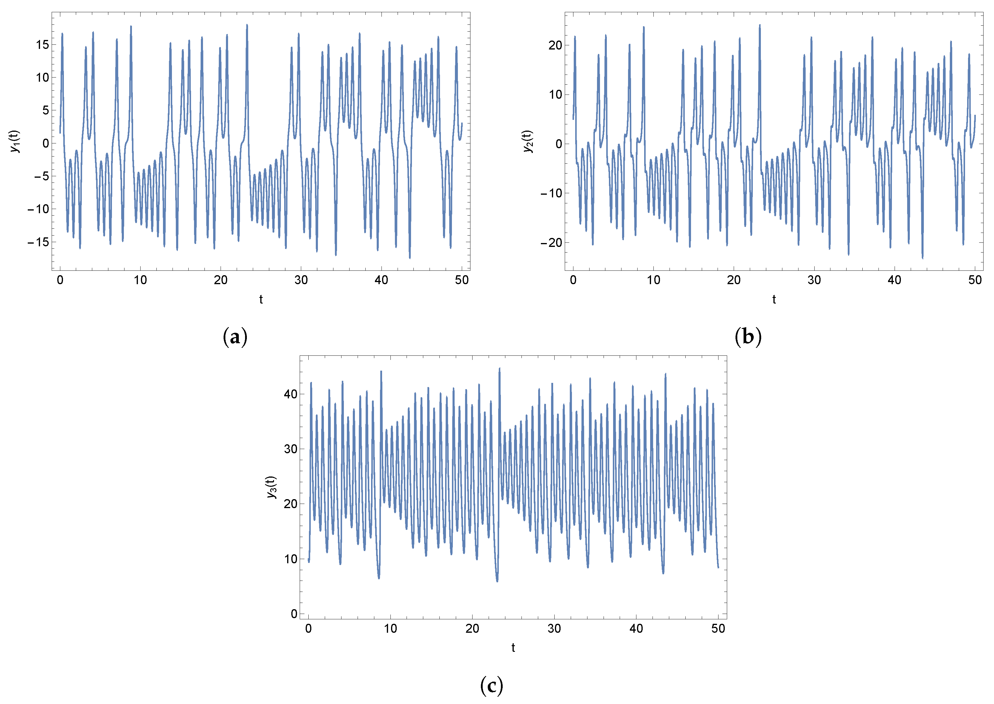
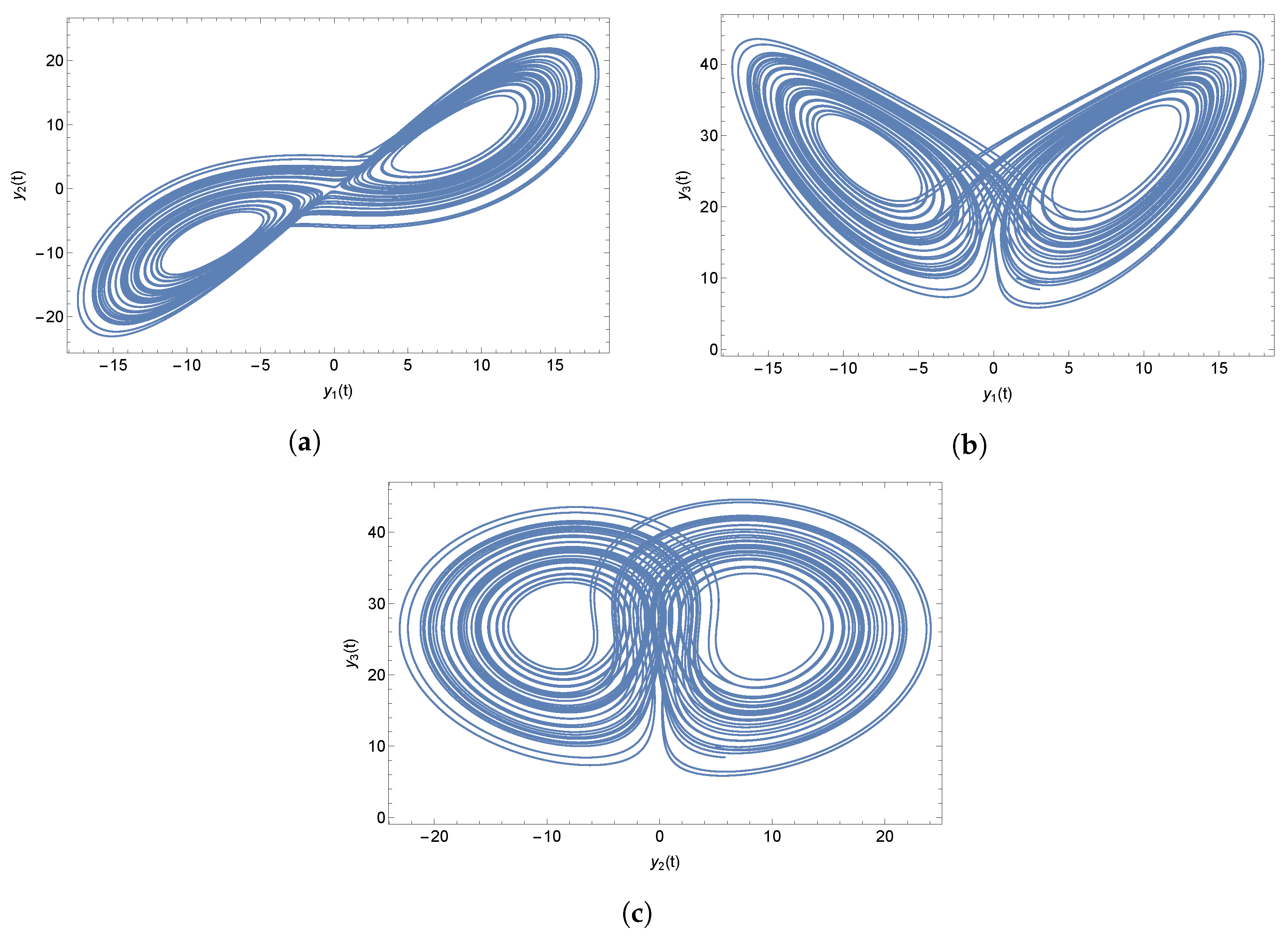
Consider the Lorenz system [18] given by

$$\begin{array}{cccc}{y}_1^{\prime }& =a(y_2-y_1),\hfill & y_1\left(0\right)\hfill & =1\hfill \\ y_2^{\prime }& =-y_1{y}_3+b{y}_1-y_2,\hfill & y_2\left(0\right)\hfill & =5\hfill \\ y_3^{\prime }& =y_1{y}_2-c{y}_3,\hfill & y_3\left(0\right)\hfill & =10\hfill \end{array}$$

The constants are $a=10,b=28,c=8/3$. With these selected constants, the Lorenz system exhibits chaotic behaviour, with the solution profiles fluctuating rapidly over extremely brief time intervals. To precisely and efficiently capture the solution, robust numerical approaches are necessary. The proposed overlapping HBM with the fewest intra-step points was employed to tackle this problem.

The parameters of the iteration scheme are given below.

$$\begin{array}{cc}\hfill {\varphi }_1(t,y_1,y_2,y_3)& =-a,{\psi }_1(t,y_1,y_2,y_3)=a{y}_2,\hfill \\ \hfill {\varphi }_2(t,y_1,y_2,y_3)& =-1,{\psi }_2(t,y_1,y_2,y_3)=b{y}_1-y_1{y}_3,\hfill \\ \hfill {\varphi }_3(t,y_1,y_2,y_3)& =-c,{\psi }_3(t,y_1,y_2,y_3)=y_1{y}_2\hfill \end{array}$$

In Figure 9 and Figure 10, respectively, the time series solutions and phase portraits for the Lorenz equation are displayed. These results were produced using OOHBM-3 with $h=0.01$ across the integrating domain [0,50]. The results are identical to those reported in numerous publications on the Lorenz system’s solutions (see, for example, [19]).

5. Conclusions

In this study, an enhancement to the conventional hybrid block methods for solving first-order equations was developed. This was accomplished by overlapping successive integration blocks after the first block. When executed on a variety of initial value problems, the resulting method, called the overlapping hybrid block method, demonstrated a significant gain in accuracy. In addition, theorems were established that demonstrate an improvement in local truncation error by an order of the step size, $O\left(h\right)$. It was also demonstrated that the proposed method is A-stable. These findings show that the concept of inserting overlapping blocks in hybrid block methods may be a profitable field of study. Further research is required to extend the applicability of the overlapping technique to other types of differential equations, such as boundary value problems, fractional-order differential equations, and differential-algebraic systems of equations (DAEs).