1. Introduction
A supermarket refrigeration system [
1] consists of a central compressor bank that, along with other process units, maintains the required flow of refrigerant (by suction pressure) to several refrigerated display cases located in the supermarket sales area. Each display case operates with an inlet on/off refrigerant valve to keep the air temperature in the display case within a range that will maintain the quality of the goods. This is a hybrid process that entails non-linear switched dynamics and discrete events, discrete manipulated variables (open/close valve and turn compressor on/off), continuous controlled variables (i.e., temperature of goods), and finally, several operational constraints.
Many processes are all-too-often designed without taking dynamic considerations into account. The design step only computes the physical parameters, size, and economic cost of the units and other system component conditions that, in the best possible way, meet the requirements of the chosen steady state operating point. This can lead to loss of performance when the process has to interact dynamically with its control system. Integrated design, however, is a technique that considers the control system of the plant and its controllability issues in the selection of plant parameters. Therefore, isolated decision-making for process and control design would result in, if not infeasible, a sub-optimal solution. A good revision and challenges in this topic can be found in references [
2,
3,
4,
5,
6].
The goods in the display case should be kept within the specified temperature bounds in order to preserve them for consumption, and suction pressure of the compressor should not be increase above a value for security issues. In addition, it is recommended to decrease the number of compressors and valves switches to increase the lifetime of these equipment and finally it is important to reduce the energy consumption of the compressors in order save money in the daily operation of the refrigeration system. According to the above objectives, the performance of a refrigeration supermarket system is evaluated by three measures, initially proposed in 38 [
5]: (i)
γcon, violation of the constraints on the air temperatures inside the display cases and at the upper level of the suction pressure. (ii)
γswitch, the number of start/stop commands sent to the compressors and the number of inlet valve switches, and (iii)
γpow, the average power consumption of the compressors. In addition, it is also necessary to consider a day/night operation of the process. So, there are six measures or responses to be minimized.
In [
7], the authors developed a predictive hybrid controller (HMPC) to control a simulation of a refrigeration supermarket system, improving the behaviour of the process compared to when traditional decentralized PI controllers are used [
5]. In this approach, certain on/off actions were considered in terms of time instants of the events, instead of using binary values in each sampling time such as, for example, mixed logical dynamical (MLD) framework presented in [
8] and used in [
8] to develop a mixed-integer model predictive Controller based in linear models to control a simulation of a refrigeration supermarket system. The approaches in [
7,
9] and more recently in [
10] circumvents the computational difficulties of solving a mixed-integer optimization problem each sampling time, reformulating the switching dynamics. On the other hand, linear models provide an inadequate representation of the non-linear dynamics that take place within refrigeration systems, which results in a mixed-integer non-linear optimization problem which is unsuitable for real-time control.
The above procedure proposed by the authors was previously applied to other process, i.e., [
11], an industrial process where continuous and batch units operate jointly: the crystallization section of a sugar factory. The process includes both continuous objectives and continuous manipulated variables, as well as those objectives related to the discrete operation of the batch units and discrete manipulated variables. This approach leads to a predictive controller formulation where discrete variables are avoided and a non-linear optimization problem (NLP) is solved online every sampling time, instead of solving a mixed-integer non-linear optimization problem (MINLP), the solution for which is much more computationally expensive.
The relation between these six indices and the configuration of the refrigeration system (number and capacity of compressors) is neither explicit nor modelled by the equations in the controller. It is, however, a consequence of system dynamics and control. Therefore, any optimal integrated design of a supermarket refrigeration system has to be performed by estimating this unknown functional relation through calculation of the indices for certain configurations. The selection of these configurations should be done in such a way that the functional models provide the most precise possible estimation of the indices. Response surface methodology (RSM) is the solution to the problem of selecting the most suitable experiments when seeking to estimate models on the basis of experimental data from a given system, [
12,
13]. RSM has been extensively used in process optimization [
14] to study and optimize critical aspects in processes that are already in operation. The variability estimation is needed, in standard RSM, as a reference to establish the model validity (lack of fit hypothesis test), the effect of the experimental factors (analysis of variance, ANOVA), the precision of the model coefficients, and the precision of the estimated response with the fitted model.
The design and modelling of computer experiments have become popular topics over recent years. Several comprehensive works, i.e., [
15], have emphasized the challenges and importance in this relatively new area. Usually, so-called space-filling designs are used to generate the necessary computational experiments. In addition, various modelling techniques have been proposed: Kriging models, (orthogonal) polynomial regression models, local polynomial regression, multivariate spline and wavelets, Bayesian methods, and machine learning methods as neural networks. Some recent examples of the application of machine learning-based computational techniques in different engineering areas are showed next. The incorporation of the solvents into process design occurs by means of a serial clustering [
16]. A neural network is used to model surface tension [
17] for the design of heat exchangers and mass transfer equipment. In [
18], the effect of temperature, pressure, and amount of graphene oxide on CO
2 capture by an aqueous solution of methyl diethanolamine is analyzed using different artificial intelligent models. The effect of fouling caused by formation of scales in the pipelines of oil and gas is modeled by a neural network in [
19]. Finally, reference [
20] is a recent review about current state and the future directions of computer experimentation in process engineering.
The design of the experiment and the surrogate model are the two key issues in computational experiments and their interaction restrict the achievable results, but, in general, both are defined in an independent manner. In fact, the theory that describes the relationship between both to develop optimal procedures for computational experimentation is scarce.
Unlike what happens in computational experiments, in RSM a link is made between the model and the design to obtain those experiments that are required to fit the model with the best quality. For this task, it is necessary to define the criteria that allows one to compare the quality of the designs proposed for an experiment before carrying it out. In RSM, it is considered that there is an experimental variability, that is to say, that if the experiment is repeated under the same conditions, a different result will be obtained; this does not happen in a computational experiment. This variability is transmitted to the coefficients of the fitted model and to the values calculated with it. Thus, once the number of experiments to be used is fixed, a design is D-optimal if the variance of the coefficients of the model is the lowest possible and is said to be G-optimal if the variance of the response is minimax in the experimental domain [
12,
13].
In a computational experiment, there is no experimental variability, but in this paper, it is shown that criterion D introduces a metric in the Euclidean space of the coefficients and criterion G in that of the response values, therefore they can continue to be used to obtain an optimal experimental design.
Extending the use of RSM methods to computational experiments has the advantage that it leads to solutions where the Euclidean distance between the response values (the six quality indices) obtained computationally and those predicted by the proposed subrogate model is minimal. This is because the response surface is calculated by least squares. In addition, RMS provides the optimal design with the minimum number of points where the computational experiments must be made.
This approach is explored and applied, for the first time, in the integrated design of a process which is a computational experiment, without experimental variability, to obtain the best configuration of the process to be installed in terms of the number of necessary compressors and their corresponding discrete capacities, considering the aforementioned control objectives and the behaviour of the process with the overall control system. Formally, the distribution of total capacity into three compressors is a mixture problem with constraints.
The paper is organized as follows. Following this introduction, the elements of the problem are described in the next two sections.
Section 2 describes the model of the process, its control by means of Hybrid Model Predictive Control, the implementation of the controller, and the indices that are to be controlled.
Section 3 describes the polynomial models for the design of response surfaces, in order to understand mixture problems, criterion D in terms of a metric in the space of the possible linear models, and criterion G as a function of quadratic loss; the section ends with a description of the procedure, in order to obtain a D-optimal experimental design. The results and discussion are shown in
Section 4, where the analysis of the six responses is performed through the desirability function. Finally, a number of conclusions and references bring the paper to an end.
2. Supermarket Refrigeration Systems
Commercial food outlets in the UK are responsible for 3% of the UK total energy consumption, while refrigeration systems represent 29% of this total [
21], so, improving the performance of the refrigeration system has a huge potential in reducing electrical usage and costs. In that paper, a model which is tuned and validated with the real operational data collected from the Refrigeration Centre is developed in MATLAB/SIMULINK and used to simulate the operation of a commercial refrigeration system in order to examine and investigate the impact of various operational parameters in this kind of systems.
It is important to consider the difficulty to control this process due to high thermal inertia, dead times, high coupling between variables, and strong nonlinearities, so many authors have developed benchmarks to design and test adequate control system, including [
1,
22].
This section lists the elements of the model that will be optimized. A detailed description of their contents may be consulted in [
7,
23].
2.1. Plant Process Description
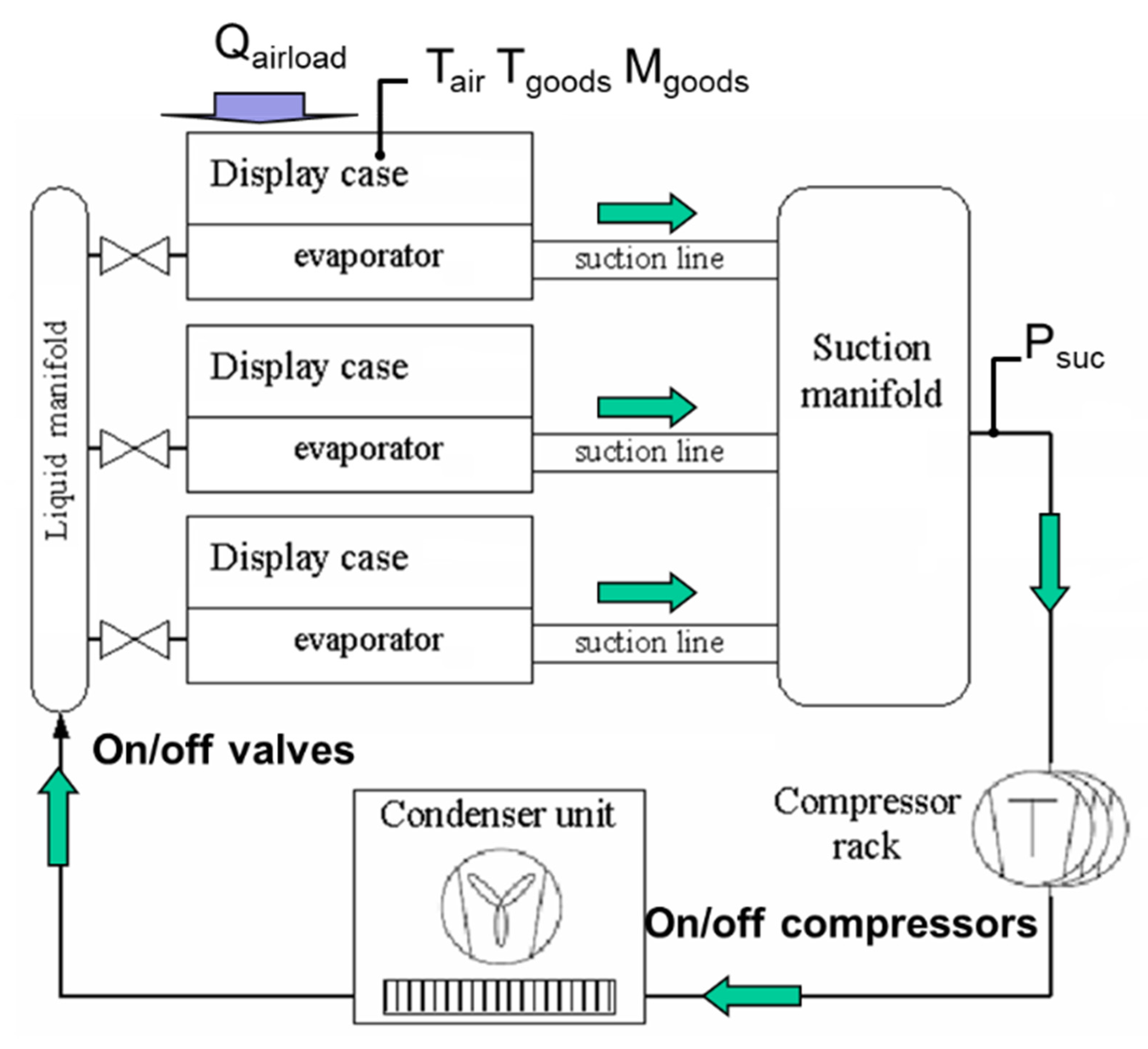
Many foodstuffs have to be kept in refrigerators to ensure that they remain fit for human consumption. In supermarkets, these are usually held in open display cases that facilitate self-service. A simplified supermarket refrigeration circuit with three display cases is shown in
Figure 1. Refrigeration of the open display cases maintains the quality of the goods that are on offer to the public. They contain an evaporator that receives the flow of refrigerant and maintains the required temperature for the goods. The other element of the system is the compressor rack, which consists of a number of compressors connected in parallel. They supply the flow of refrigerant to the system by compressing the low-pressure refrigerant from the suction manifold, which receives the vapours returning from the display cases. The compressors maintain a constant pressure in the suction manifold, thus ensuring the desired evaporation temperature. The dynamic in the suction manifold is modelled by only one state: suction pressure (
Psuc).
The refrigerant flows from the compressors to the condenser and further on to the liquid manifold. The evaporators inside the display cases are fed in parallel from the liquid manifold through an expansion valve. The outlets of the evaporators lead to the suction manifold and back to the compressors, thereby closing the circuit.
A temperature sensor is located inside the display cases, which measures the air temperature
Tair close to the goods. This temperature measurement is used in the control loop as an indirect measure of the temperature of the goods. Furthermore, an on/off inlet valve is located at the refrigerant inlet of the evaporator, which is used to control the temperature in the display case. Finally, in
Figure 1, the arrows indicate the circulation of the refrigerant in the refrigeration system.
2.2. Typical Decentralized Control Structure
The
Tair in the display cases is controlled by a hysteresis controller (1) that opens and closes the inlet valve.
The suction pressure controller is normally a Proportional Integral controller (PI-controller) with a dead band (±
DB) around the reference of the suction pressure (2) where
e(
t) is the control error and
uPI is output from the PI-controller. If the compressor capacity is a discrete value, then the applied control signal
ucomp,i (
i = 1, 2, …,
nc) is obtained as follows:
where
Ccomp,i is the
i′th compressor capacity (
) and
nc is the total number of compressors installed. The dead band ensures that the integration is stopped as long as the suction pressure is within the dead band. When the pressure exceeds the upper bound, the integration is started and one or more additional compressors are turned on to eventually reduce the pressure, and vice-versa when the pressure falls below the lower bound. Hence, moderate changes in the suction pressure and small biases from the reference do not initiate a compressor switching.
In the supermarket, many of the display cases are similar in design and work under uniform conditions. As a result, the inlet valves of the display cases are switched with very similar switching frequencies. The valves therefore tend to synchronize, leading to wide oscillations of suction pressure and temperatures, with the consequence that many of the controlled variables are out of control, and the compressors wear out due to frequent starts/stops and synchronization.
2.3. Hybrid Model Predictive Control, Advanced Process Control
In response to the aforementioned problems that are inherent to decentralized control, a centralized Hybrid Model Predictive Control, HMPC, has been proposed in [
7] but maintaining in the low level only the PI controller for suction pressure (2). HMPC uses a rigorous non-linear continuous-time model to describe the dynamic of the refrigeration system. The main emphasis in the modeling is on the suction manifold and the display cases, which contain the most relevant dynamics for controlling them. The model considers the features of the refrigerant and the compressor. The compressor’s capacity in most refrigeration systems is a discrete value, as compressors can either be switched on or off. In addition, the system dynamics based on first principles are considered as well as the manipulated variables that correspond to the opening/closing of the valves in each display case. A new parameterization converts these integer decision variables into real decisions
and
, that is, the time instants when the integer variable
I changes its value. This approach allows us to use conventional non-linear optimization techniques (in terms of real variables) instead of mixed-integer non-linear programming, decreasing the complexity of the optimization procedure and saving computation time.
The following variables are considered from the standpoint of system control, where i refers to a specific display case, and n is the total number of display cases:
The
controlled variables are, respectively, the suction pressure (
Psuc) and the air temperature (
Tair,i) in each display case (
i = 1, …,
n). They are measured, as indicated in
Figure 1, for each display case.
The on/off manipulated variables are the opening/closing of the inlet valves of the display cases.
The non-measured disturbances are the heat load on the display cases (Qairload) and the variation in mass of goods (Mgoods,i) inside them.
The temperature of the goods (Tgoods,i) in each display case are non-measured variables that are controlled indirectly using air temperature.
Several constraints apply to suction pressure (Psuc) and to air temperatures (Tair,i).
In the structure of
Figure 1, composed of 3 display cases, a non-linear model has to be solved that has 888 variables and 67 equations in the case of two compressors (16 of which are differential equations). In the case of three compressors, there are 889 variables and 69 equations of which 16 are also differential equations.
The model describes the behaviour of the system at each future point, based on the present situation,
t = 0. The future action of the valves (open/close or no change) is based on the mean expected behaviour of the controlled variables up until a temporal horizon
Tp. The objective is to maintain the controlled variables “close” to the reference value, minimizing a cost function
J, defined by:
where,
is the reference value of the suction pressure in the controller PI,
and
are the minimum and maximum acceptable values for the temperature in each display case, and α
i (
i = 1,…, 1 +
n) is the weight of each addend in Equation (3).
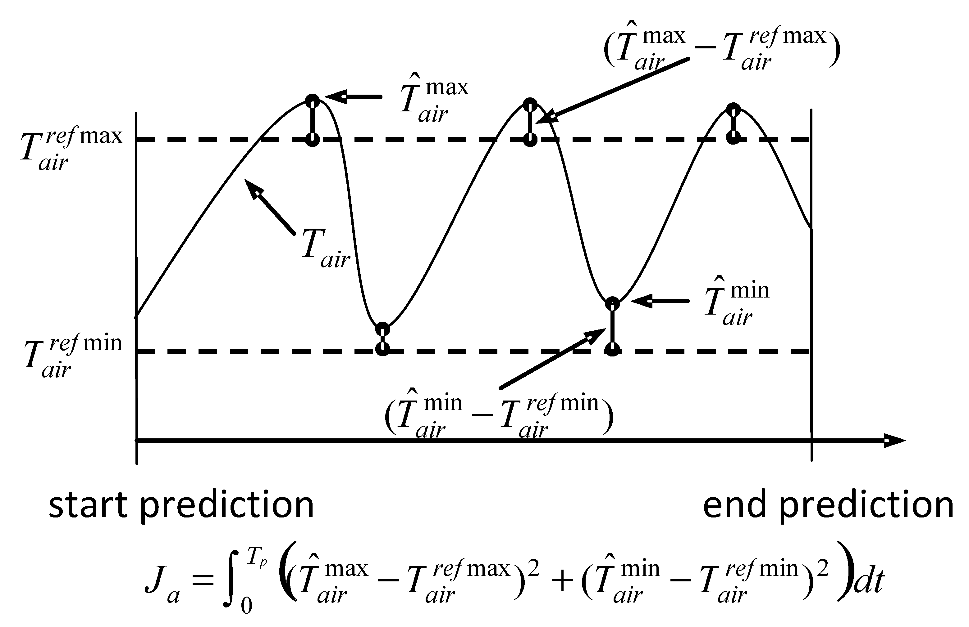
Although HMPC does not manipulate the compressors, the first term of Equation (3) penalizes the difference between the suction pressure and its reference. Each of the terms that constitute the second part seeks to maintain a stable periodical pattern of air temperature in the display cases. Due to the oscillatory nature of air temperature, the idea is to obtain waves with a certain constant amplitude fixed by the maximum and minimum values allowed
and
(desired amplitude =
), see
Figure 2. The permitted level of oscillation is between
and
, while
and
are the maximum and minimum values reached by
Tair,i throughout the prediction interval.
2.4. Controller Implementation
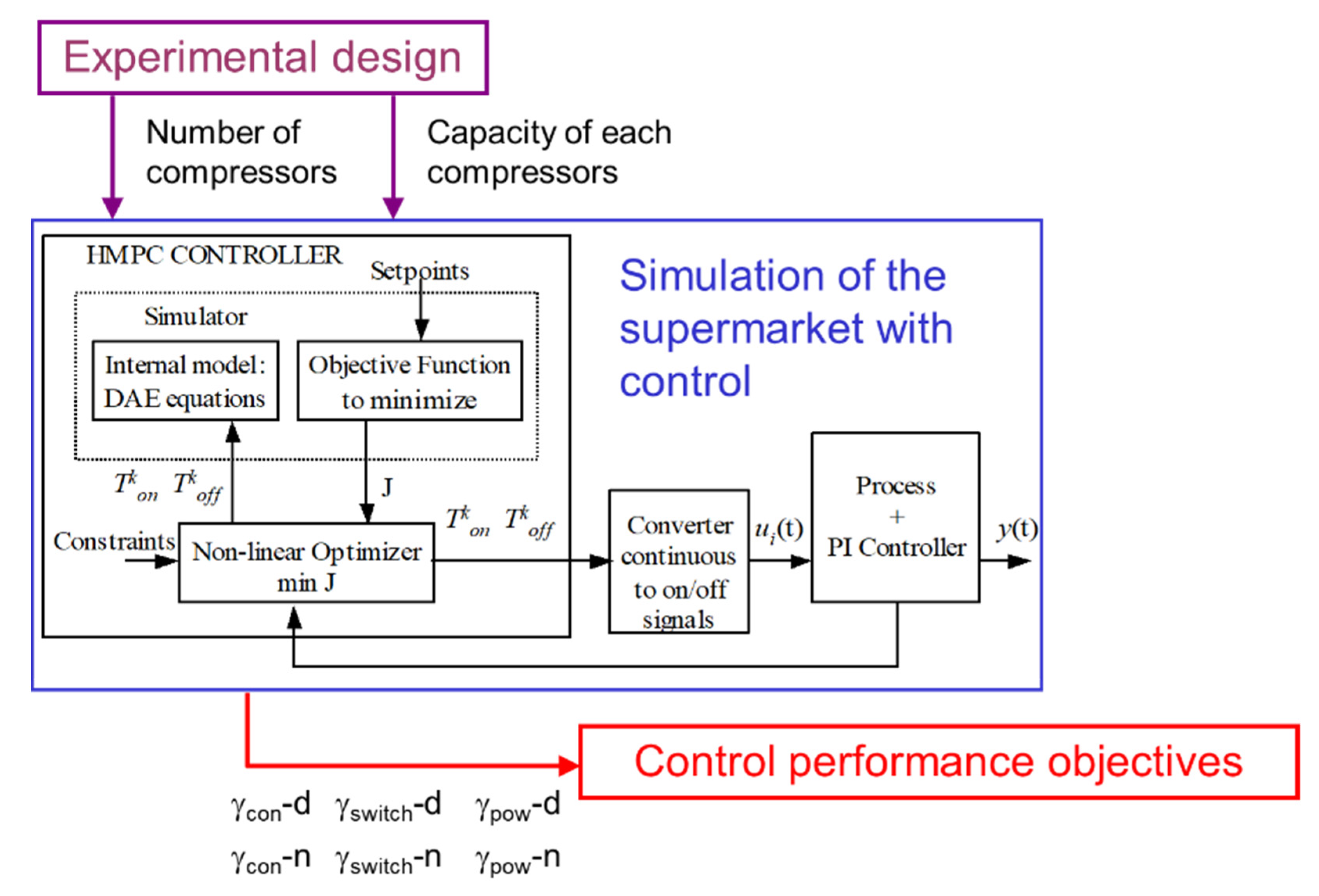
The aim of the HMPC is to minimize J, Equation (3), considering the system dynamics, with respect to the decision variables related with the opening/closing position of the valves in each display case and with those the starting/stopping of each compressor.
The resulting non-linear optimization problem is solved each sampling time using an SQP algorithm [
24] implemented in a commercial library NAG for C [
25] following the schematic of
Figure 3, which corresponds to a sequential approach where the cost function,
J, is computed by the integration of the dynamic internal model. The simulation package integrates the equations of the internal model equations along the prediction horizon,
Np, taking as initial conditions the current process state and evaluating the formulated cost function,
J, at the end of the integration.
Both dynamical models, supermarket process plus PI controller and the internal model were coded in the modelling environment EcosimPro [
26]. This is a modern simulation software which allows combining DAE equations with events performing a correct integration in spite of the model discontinuities. In addition, it can generate C++ code corresponding to the simulation. Taking the advantage of this capability, the code of the internal model was embedded with the nonlinear optimizer in the HMPC controller which has been programmed in C++.
From a technical point of view, it is necessary to add a real/discrete converter between the controller and the process, see
Figure 3. HMPC calculates the exact time instants,
and
, of changes for each on/off manipulated variable, and the converter transforms these times into a discrete manipulated signal when the events will occur. In other words, the application of the on/off signals is decoupled from the sampling time.
2.5. Control Performance Objectives
The general control objectives are: meet the constraints on refrigerator temperature and on suction pressure, minimize the number of times the compressors are turned on/off, and minimize the consumed power. Accordingly, various indices are defined in accordance with each control objective, in order to evaluate the behaviour of the controller. According to reference [
1], the three initially proposed indices are,
γcon,
γswitch, and
γpow.
2.5.1. Constraints
The index
γcon may be interpreted as the mean of the square of violations per second of the constraint, both with respect to suction pressure,
, and maximum,
, and minimum,
, temperatures, in each case.
where,
is the function that expresses the violation of constraints in suction pressure in time
t and
corresponds to the violation of the constraint in the
i-th display case in time
t.
2.5.2. Switches
One of the main objectives is to reduce the number of starts and stops of the compressors. In general, the useful life of a compressor is approximately 100,000 starts/stops, therefore by reducing that number in daily operation, the life of the compressors may be extended. On the one hand, the cost of opening and closing the valves is 100 times less than the cost associated with the compressors. In other words, the operation of the valves is less critical than the operation of the compressors. The following index,
γswitch, is introduced to measure the behaviour of the controller with regard to these stops and starts:
where
Ncomp(
t) indicates the number of compressors that have been stopped and started within time
t, and
Ndisp(
t) also refers to the number of valves that have been opened and closed within the same time
t. Therefore,
γswitch is the number of compressors started up and stopped per second, where 100 changes in the valves count as a change of compressor.
2.5.3. Power Consumption
The compressors consume the largest portion of energy in a refrigeration system, which is why it is important to reduce this consumption. Average consumed power,
γpow, is the most appropriate index to measure this consumption.
where
Powcomp(
t) is calculated, as detailed in [
27], from volumetric flow and the enthalpies of the refrigerant considering isoenthropic efficiency.
In supermarkets, during the night-time, refrigerators are covered with “night covers”, which considerably reduce the heat load, Qairload, and the constant mass flow to the suction collector. The model can include the change from day to night, modifying the new values of Qairload and fref,const within a set time, which are considered measurable perturbations that do not have to be estimated. As from that moment, it is necessary to introduce new indices because increases as well as its reference and its lower limit.
There are therefore three indices with which to evaluate daytime behaviour: γcon-d, γswitch-d, and γpow-d and another three for night-time behaviour γcon-n, γswitch-n, and γpow-n. It is clear that the smaller the value of each one, the better the refrigeration system performs.
The relation between the minimum of these indices and the structure of the refrigeration system (number and capacity of the rack of compressors) is neither explicit, nor is it modelled by the equations of the controller, although it is the consequence of the system dynamic and of its control. Therefore, optimization of the structure of the refrigeration system must be done through the estimation of the functional relation derived from the calculation of the indices for some configurations.
Figure 3 shows a schematic diagram of the computational experiment: the number and capacity of compressors is fixed, the process and its control are simulated over a given period of time that includes day/night changes, and the six indices are evaluated.
3. Experimental Design for Mixture Studies
If
q is the number of compressors and
xi is the fraction of the total power of each one, the configuration of the compressor rack will be defined by the variables
xi that satisfy:
The six responses or indices of interest,
γl, are, for optimization purposes, functionally related to the proportions of power:
In an attempt to study the relationship in Equation (10) for each index, different combinations of the components will be tested to analyse the variation of each γl by changing the rack configuration (x1, x2, …., xq). These are the individual experiments on the basis of which the function proposed in Equation (10) is estimated. After verifying the validity of the estimated function, which substitutes the unknown functional relation, the researcher may be interested in identifying whether a configuration exists that will yield optimum responses, or simply in gaining a better understanding of the whole system, through the joint analysis of the behaviour of every possible configuration.
Functions
fl(.) in Equation (10) are the surrogate model of all equations used to describe the process and its HMPC controller shown in
Section 2 (corresponding to the blue box in
Figure 3). The surrogate model is a regression model which is trained with results obtained with the computational model evaluated in certain points of the experimental domain (
ED). According to Gramacy [
28], a good surrogate model has to provide an estimation of the response in other points of the experimental domain where the computational model has not been evaluated. In this way, the surrogate model should be much simpler and faster than the original one but can be used for the same purposes, i.e., finding an optimum.
The response surface methodology allows us to select the number and the characteristics of the experiments needed to obtain the most accurate estimation. However, as it cannot be used directly for mixture experiments, because of the equality constraint in Equation (9), most of the research into mixture problems has been focused on developing models and designs to explore the whole or part of the mixture space.
3.1. Experimental Domain
The experimental domain is formed by the set of possible configurations. Theoretically, all points (x1, x2, …., xq) under the constraints of Equation (9) are a simplex in the q-dimensional space. As already indicated, compressor capacity is a discrete-value and several practical constraints are imposed, therefore the experimental domain is a discrete subset, ED, which does not cover the entire simplex.
3.2. The Model
A surrogate model is chosen to model the response, along with the ED candidate design points that are selected in the design and analysis of a mixture experiment, in an irregular experimental domain. From this list of candidate design points, a computer algorithm selects the design points according to the chosen optimality criteria.
Scheffé canonical polynomial models are usually used to represent the response [
29]. The surrogate models are the result of incorporating the mixture constraints into polynomials. The simplex–centroid design presented is a widely used model that has
p = 2
r− 1 terms (all the different crossed products) where
r is the degree of the polynomial. For example, the canonical polynomial up to grade four is given by the following expression:
3.3. Optimality Criteria
This model has p parameters to be estimated by taking observations in the constrained ED space. An appropriate rack configuration must be chosen to calculate the six indices, so as to ensure that the data will contain the desired information. In other words, the experimental results must enable the coefficient estimation of a model that can be used for accurate prediction at any point of the domain of interest, having established its suitability to represent the evolution of each index γl(l = 1, 2, …, 6).
The simplest strategy might be to conduct the experiments on all the candidate points of ED. However, reducing the number of experiments may be a relevant requirement worth further consideration. Should this be so, then the objective is to select a subset of points from ED which will provide precise estimates of the parameters in the model, given in Equation (11). Some quantitative criteria are needed to be able to compare various experimental designs before selecting an optimum design.
After selecting
N p experiments from
ED, the values of each index are calculated for use in the system of linear equations:
where
ν is the calculated vector of
N values of each response,
Χ is the
N ×
p matrix of mixture component proportions and their respective interactions (design matrix),
β is the vector of
p coefficients to be estimated, and
ε is the vector of
N errors that arise because the supposed model reflects an estimated and not a true relation between the index and the rack configuration.
The least squares solution of system (12) is the set of coefficients (13) that provide the minimum quadratic error between the true values
ν and those calculated by the model. In our problem, the experiment is computational, so
ε does not have the habitual random meaning, but is a measure of the error caused by using the Equation (11) instead of the true, unknown, functional model. Therefore, the procedures that have been developed for random errors also have a geometrical sense and, as shown in the next section, maintain their usefulness.
where
T stands for transpose matrix and s
2 in Equation (14) is the normalized mean of the quadratic loss function:
Choosing a design is always associated with choosing particular settings in each row of Χ that, in some way, thus reduce the determinant of matrix (ΧTΧ)−1.
3.3.1. D-Criterion
The least squares fit also provides the following distance in the space of possible vectors,
β, of solutions for Equation (10):
Therefore, any neighbour of radius
k, for
b, is
. The determinant of
XTX is inversely proportional to the square of the volume of
. A small |
XTX| implies a poorly estimated model, because there are many other models in the corresponding neighbour with the same
k. The moment matrix
M is considered in order to be able to compare designs of different size
N, the determinant of which is
So, a D-optimal design is one in which the determinant of the moment matrix is at a maximum.
3.3.2. G-Criterion
The normalized mean of quadratic error, Equation (14), is translated to the estimated response,
, by means of the model fitted at any point,
x, of the experimental domain. So, this loss function
d(
x)s
2, may be computed, where:
and its maximum value,
dmax, may therefore be known.
A design is called
G-optimal when
dmax reaches the minimum value. On the other hand, appropriate and efficient designs in terms of
D-optimality have been proposed in the literature for the whole
q-simplex. The simplex lattice designs are
D-optimal for first and second-order Scheffé canonical polynomials [
30,
31]; the simplex centroid design [
32] is
D-optimal for the special cubic model of Equation (11). If the region of interest is a convex, irregular hyperpolyhedron, as in our case, the optimal design differs considerably for each specific situation. In situations like these, optimal design theory becomes an indispensable tool to guarantee design efficiency that is as high as possible in terms of a well-defined optimality criterion, such as
D-optimality for parameter estimation or
G-optimality for predicted response estimation.
3.3.3. Obtaining a D-Optimal Design
The two aforementioned criteria allow us to design a strategy to select the ED experiments that will be used to estimate the proposed model.
Step 1. Establish whether a subset of experiments, N < card(ED), exists that will provide an accurate estimation of the proposed model.
Set the minimal value, NI, such that N NI p (since the number of coefficients in the model is p) and the maximal value, NF, such that N NF card(ED).
Select an optimum experimental design for fitting the assumed
p-term model from all the possible designs of size
N based on the
D-criterion, by means of a specific algorithm. The number of different experimental #
ED designs is given by:
such that a direct search is computationally unfeasible.
Repeat this selection for different values of N (NI N NF) to obtain the D-optimal solution set.
Step 2. After D-optimal experimental designs have been generated the question of what design or designs would be the best choice must be answered. For this purpose, the G-criterion should be considered, which is the value of dmax over the region of interest. A rule of thumb is to consider only designs with dmax ≤ 1, because in this case the loss function for the response is not inflated by the effect of the design (17).
In this work, the
D-optimal design was obtained with the software NemrodW [
33], which uses a row-exchange algorithm designed by [
34] and modified by [
35,
36]. NemrodW was also used for fitting the surrogate models and data analysis.
A description of the response surface methodology that treats optimality criteria and mixture designs can be seen in [
13,
37], respectively. Text books with more of a technical content on the response surface may be found in [
12] and on mixtures design, in [
29]. However, the analytical justification of the validity of the
D and
G-criteria is shown for the first time in this work, as well as their use together with mixture design in problems of computational experiments, in which there is no experimental variability. This approach differs from the standard “space filling” method for computer experiments with compositional data (see, for example, [
15,
38]), because the model that will be used to make the fitting is not taken into account in space filling methodology.
4. Results
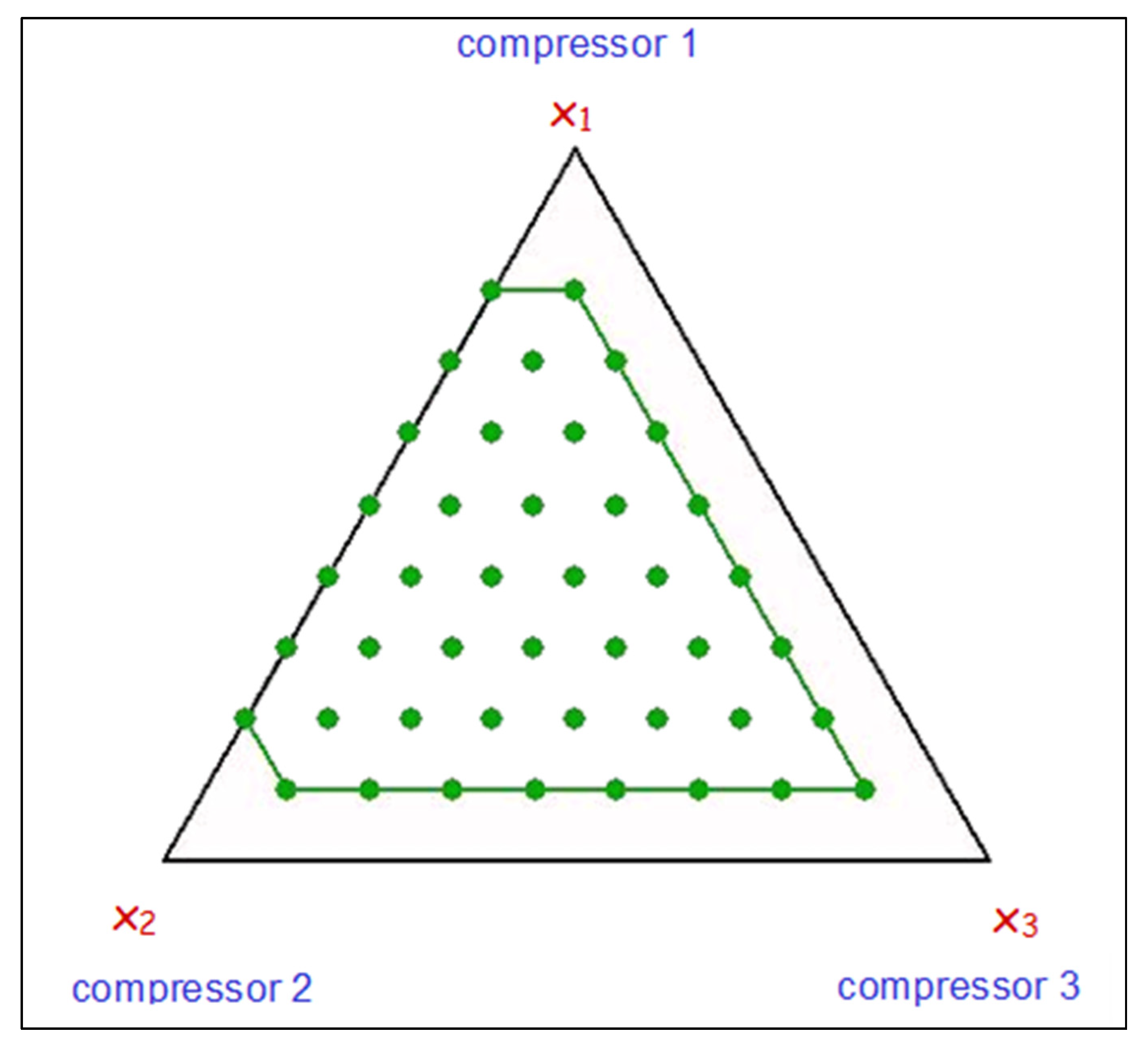
The experimental domain is a discrete space in a mixture space with three components
xi (
i = 1, 2, 3), which are their relative capacities. The constraints are: (i) The number of compressors: two or three. (ii) The maximum power of each compressor is limited to 0.8. (iii) The increases in power can only be 0.1 for the compressor. These constraints are formally stated in the system of Equation (19).
in such a way that the experimental domain consists of 43 configurations (see
Figure 4).
The proposed model for each of the indices
γl (
l = 1, 2, …, 6) is the special cubic model of Equation (11) with
q = 3.
which only has seven coefficients, such that it is necessary to know the value of the responses for seven configurations other than the compressor rack.
The validity of this model would have to be evaluated, comparing the results with those obtained from the polynomial model.
Applying the procedure described in
Section 3.3.3 yields the
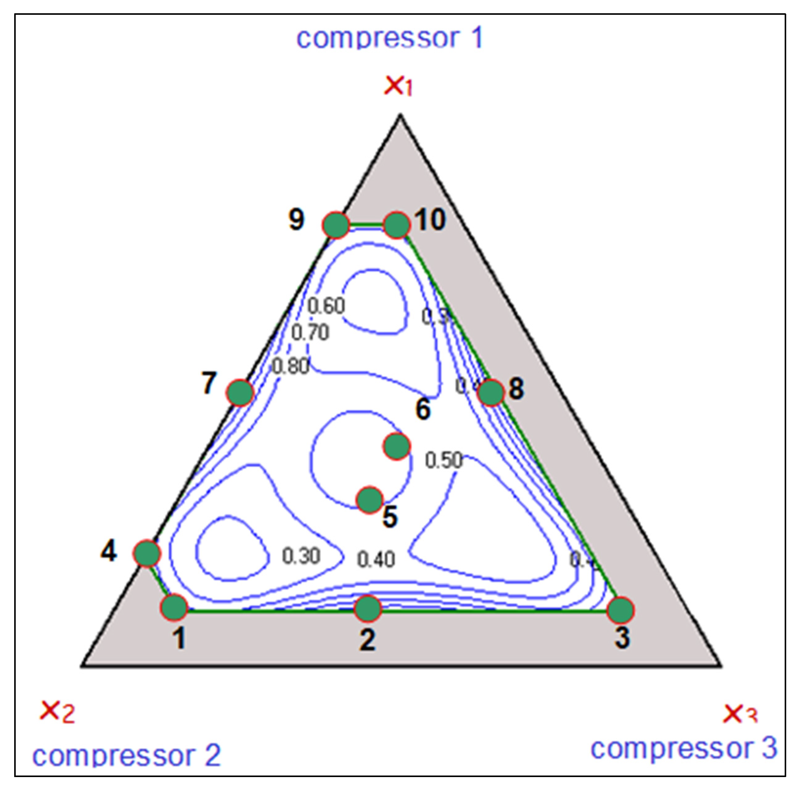
D-optimal design of
Figure 5, formed by ten experimental points. The level curves of the variance function
d(
x1,
x2, x3) =
d(
x) (17) are also shown in the figure. These values are in the order of 0.5 in the centre of the experimental domain, less than 0.4 in large zones close to the vertices and less than 1.0 across all of the experimental domain.
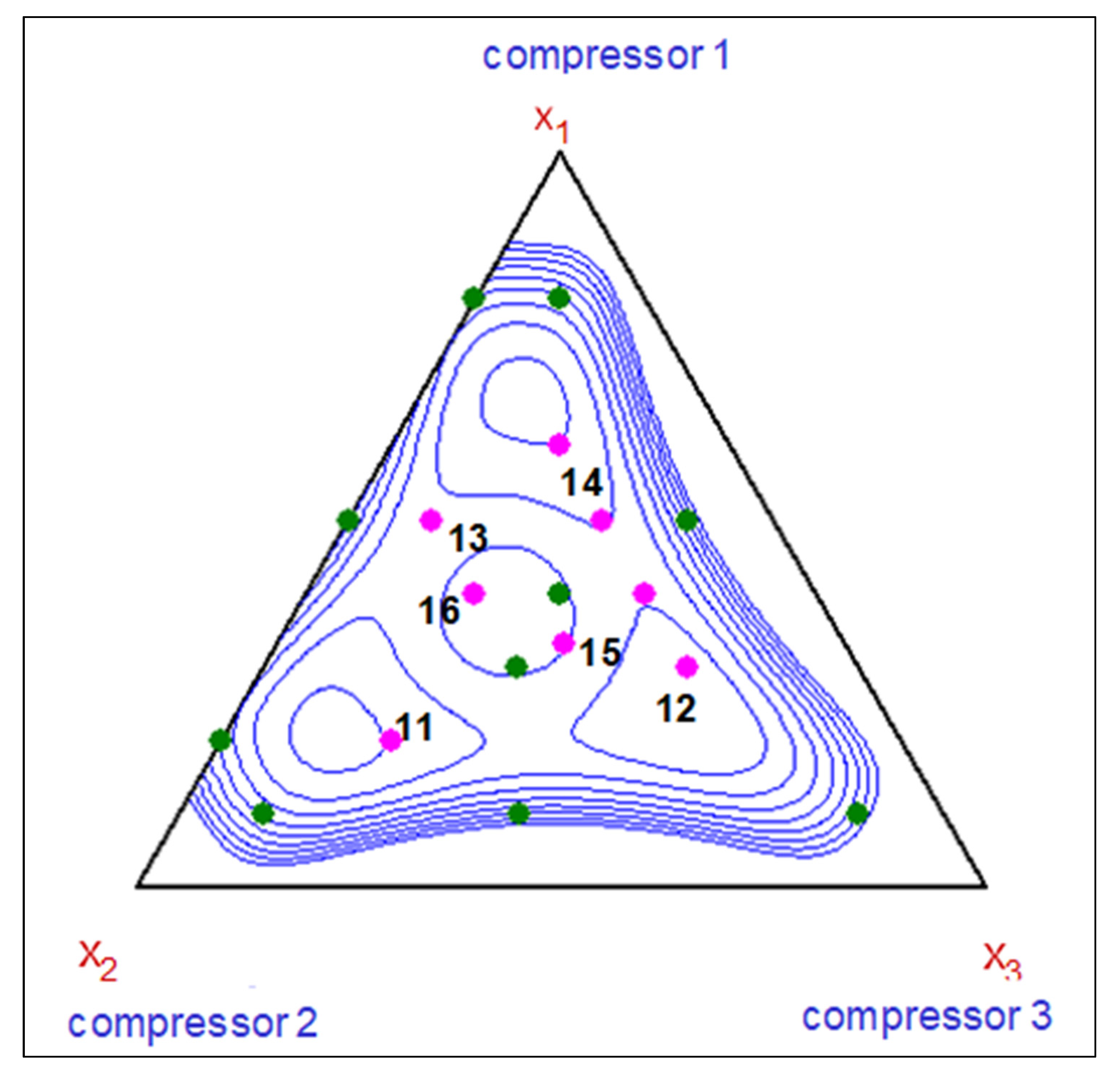
As these are computer experiments, the habitual procedure of making experimental replicates and verifying the statistical significance of the model and the lack of fit through variance analysis cannot be applied. Thus, the validity of the proposed model will be confirmed through the six-point test shown in
Figure 6.
The four experiments furthest from the centre (experiments 11, 12, 13, and 14 in
Figure 6) were selected from among those needed to enlarge the
D-optimal design in
Figure 5 to a
D-optimal design for a four-order model, Equation (11). The distribution of power (0.33, 0.33, 0.34) in experiment 15, despite not forming part of the experimental domain, was also considered, because it had been used in previous theoretical studies, and finally the distribution (0.4, 0.4, 0.2) in experiment 16 fulfils the purpose of completing the central zone of the design together with experiments 5 and 6.
Table 1 shows the experimental points and the result for each of the six variables in the 10 points of the design (1–10) and in the 6-point test (11–16).
4.1. First Model
The model of Equation (20) was fitted with the data on the first 10 experiments from
Table 1, to each of the indices
γl (
l = 1, 2, …, 6). Moreover, the coefficient of determination
R2 was calculated, which is the percentage variability of each index explained by the model; in other words, it is a measure of the adherence of the fitted model to the true values.
R2 is respectively equal to 46.6 and 60.0% for the variables
γcon-n and
γpow-n, such that the synergic model is not sufficient to reproduce those two indices.
R2 varied between 95.0 and 99.6% in the fitted models for the four remaining variables that are shown in
Table 2. The value
s is also noted, which is the square root of the value of the Equation (14) for each model. It expresses the minimum value of the normalized quadratic loss function reached for each index.
When these models are applied to the six-point test, it is possible to decide whether the predictions of the model are compatible with the experimental results. Each value calculated with the model
has a mean uncertainty, as a consequence of not using the true model derived from Equation (12) by the following expression:
Thus, the difference in each test point x may be expressed as , a normalized difference to take into account the position of the point in the experimental domain and the uncertainty caused by using a model that does not exactly reproduce the physical phenomenon.
Table 3 shows the 24 values of
difn (six-point test by four models). Only three of these exceed the value of 3.8 such that
and
may be considered different. They correspond to experiment 11 for variable
γcon-d, experiment 13 for
γpow-d, and experiment 16 for
γswitch-n. On the basis of these results, it may be accepted that the models are valid and a second model will be fitted.
4.2. Second Model
In this case the model of Equation (20) was made with all the available points (1 to 16 of
Table 3) to explore the response surfaces of the four fitted responses. Once again, the models corresponding to
γcon-n and
γpow-n have a lower value of R
2 (52.8% and 41.6%, respectively) whereas the other four are acceptable.
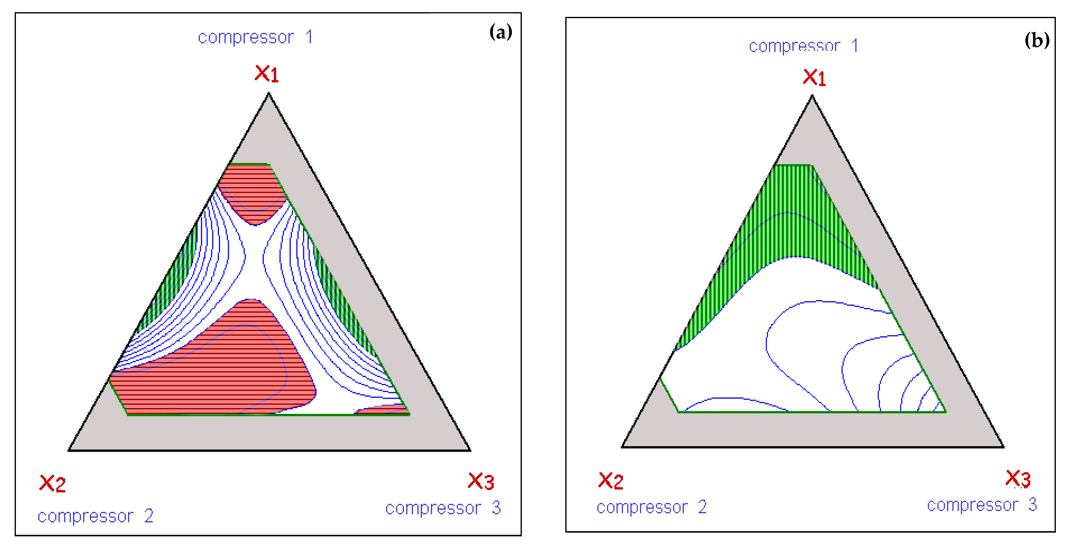
Figure 7 shows the level curves in the experimental domain for the two fitted responses
γswitch-d,
Figure 7a and
γswitch -n in
Figure 7b.
A value equal to or less than 0.03 is considered optimal for these variables (
γswitch-d and
γswitch-n) and any value over 0.10 is absolutely rejected. The acceptable region is marked in the figure with vertical stripes and the non-acceptable ones with horizontal stripes. It may be observed that the distribution of compressor power has to be completely different according to whether we consider system behaviour in the daytime or in the night-time. It is sufficient to install two compressors of similar power (50, 50, 0) or three compressors with a different distribution (40, 10, 50), to achieve the optimal response during the day,
Figure 7a. Alternatively, any configuration in which the first compressor contributes 60% or more of the power, regardless of how the remaining power is distributed between the other two compressors is sufficient for the night-time. In addition,
γswitch-n is always maintained below 0.10 whatever the power distribution.
The other two daytime variables γcon-d and γpow-d follow a very similar behaviour in the form of γswitch-d.
It is therefore necessary to look for a “compromise” configuration in the distribution of power between the three compressors.
4.3. Individual Desirability and Global Functions
The controllability of the process is considered sufficient if the six responses—
γcon-d,
γswitch-d,
γpow-d,
γcon-n,
γswitch-n, y
γpow-n—stay below certain values and insufficient if one or various values exceed certain preset limits. In particular, the two responses
γcon are considered valid (desirability 1) if they are less than 0.03 and non-acceptable (desirability 0) if they exceed the value of 0.07. The desirability function has a linear variability between both values (
γcon is for
γcon-d and
γcon-n). Thus, the function of individual desirability is:
The desirability function is considered for both
γswitch (
γswitch is for
γswitch-d and
γswitch-n):
In the case of
γpow-d, it yields:
where as for
γpow-n, we have:
The search for configurations that maximize desirability is performed in two stages:
Joint desirability,
D(
x), is constructed for the four empirically modelled variables as the geometric mean of the four individual desirabilities described above:
Having identified the region of maximum joint desirability, the individual desirabilities of the other two responses, γcon-n and γpow-n, are calculated by applying Equations (22) and (25) to the experimental values of the points belonging to the area of maximum desirability.
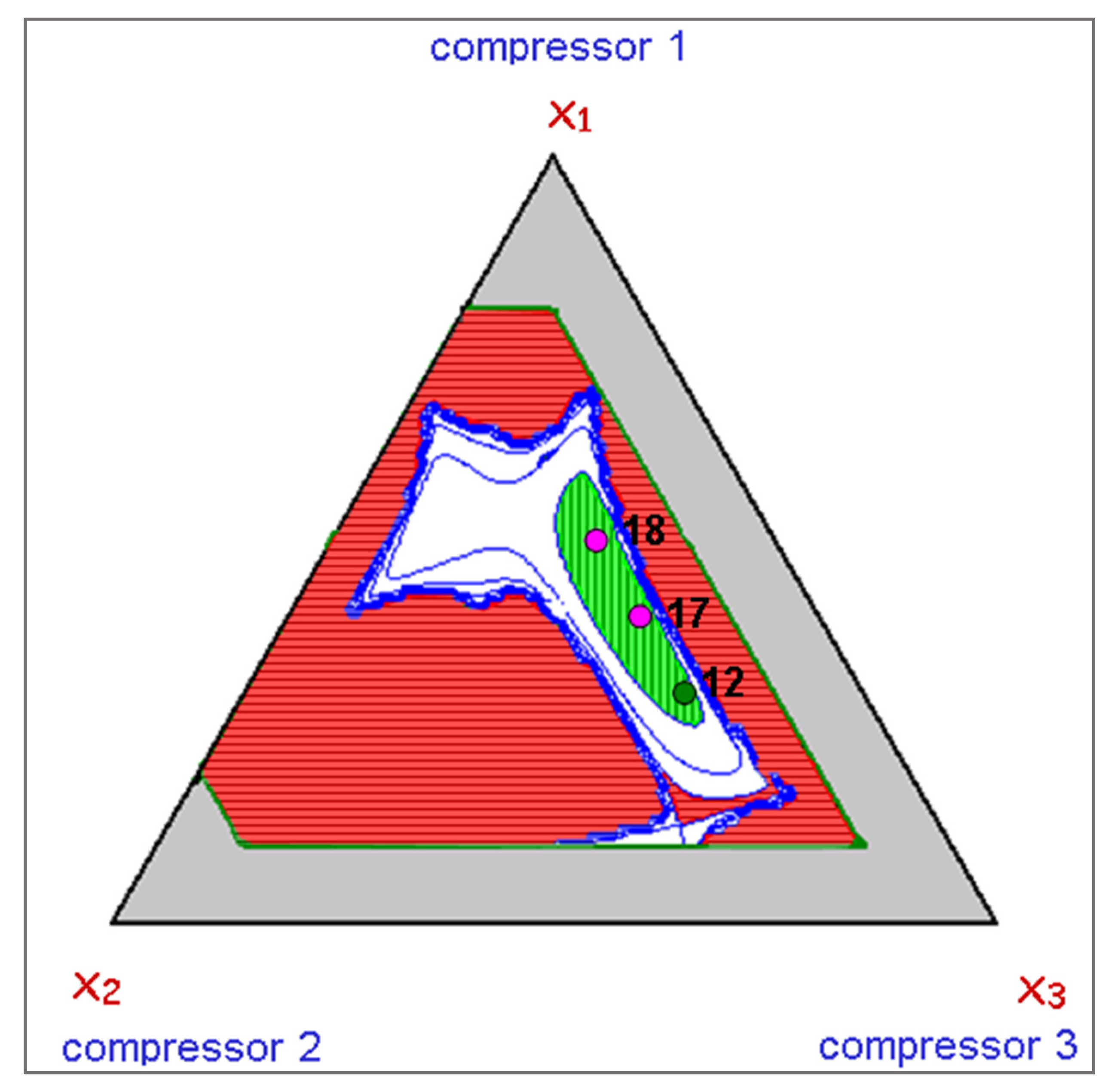
The result of stage (1) is shown in
Figure 8. The horizontally striped zone (in red) has a joint desirability of 0; in other words, it fails to comply with one or more of the four acceptable threshold values for the responses:
γcon-d,
γswitch-d,
γpow-d, and
γswitch-n. The vertically striped zone (in green) has a global desirability of between 0.6 and 0.7.
Only three points of the experimental domain are within it: the aforementioned experiment 12 from
Table 1, 17, and 18. Simulation results for these two new points are also shown in
Table 1.
Joint desirability has been calculated for these three points, taking the experimental value transformed into desirability for the two non-modelled functions: taking
dγpow-n (
x12) = 0.06,
dγpow-n (
x17) = 0.66 and
dγpow-n (
x18) = 1.0, and, in addition,
dγcon-n (
x12) =
dγcon-n (
x17) =
dγcon-n (
x18) = 1.0 Combining these results with those of desirability obtained through Equation (26), gives us a global desirability equal to 0.41, 0.67, and 0.70 for experiments 12, 17, and 18 of
Table 1, respectively. In consequence, the most suitable option is the distribution of power in the three compressors (50, 20, 30) shown in experiment 18.
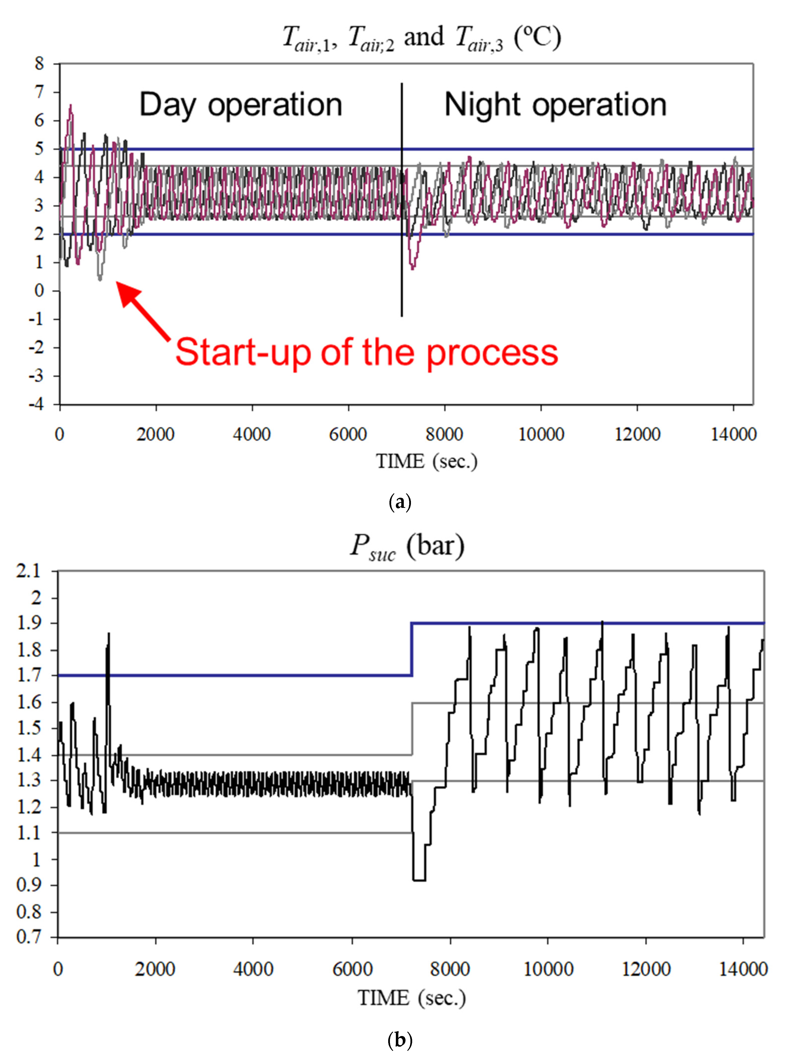
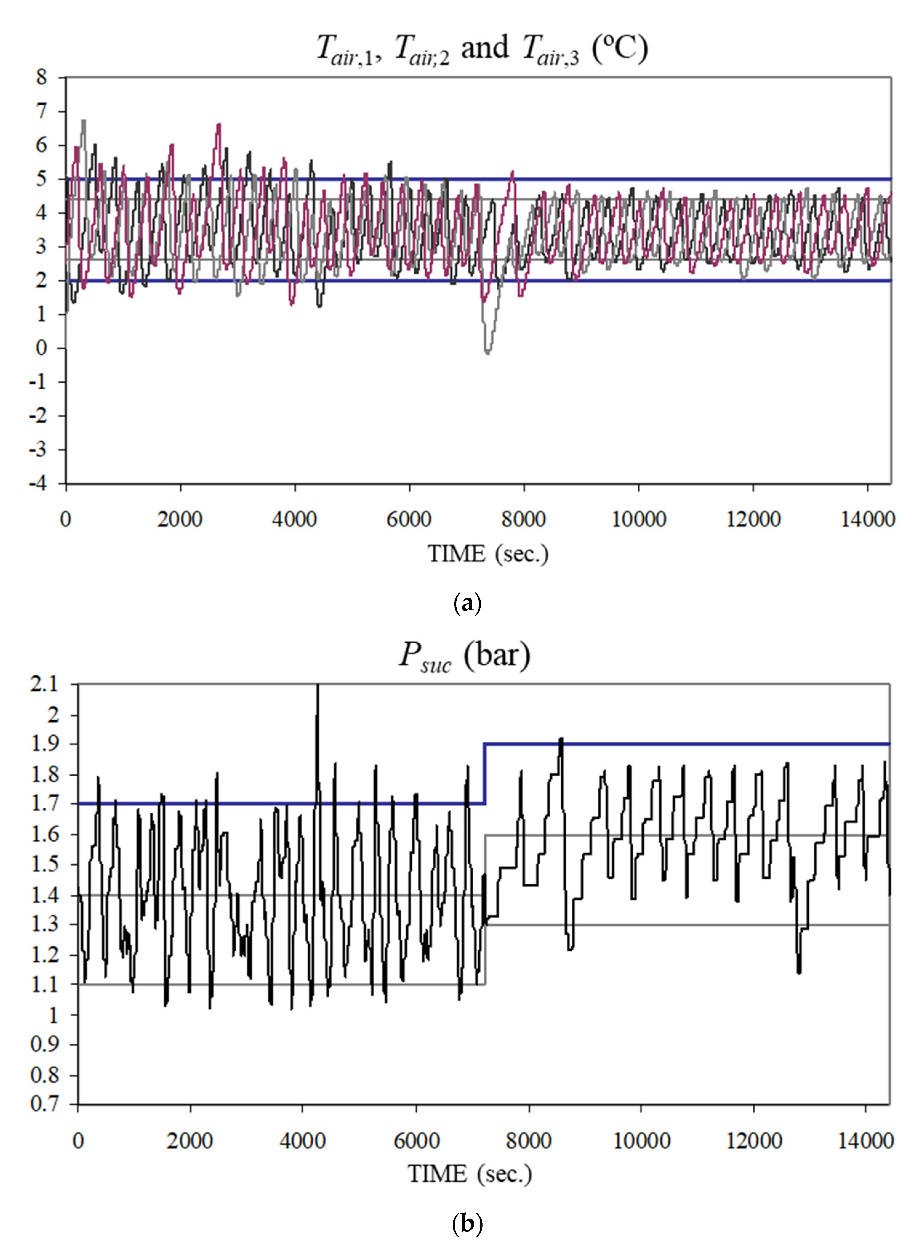
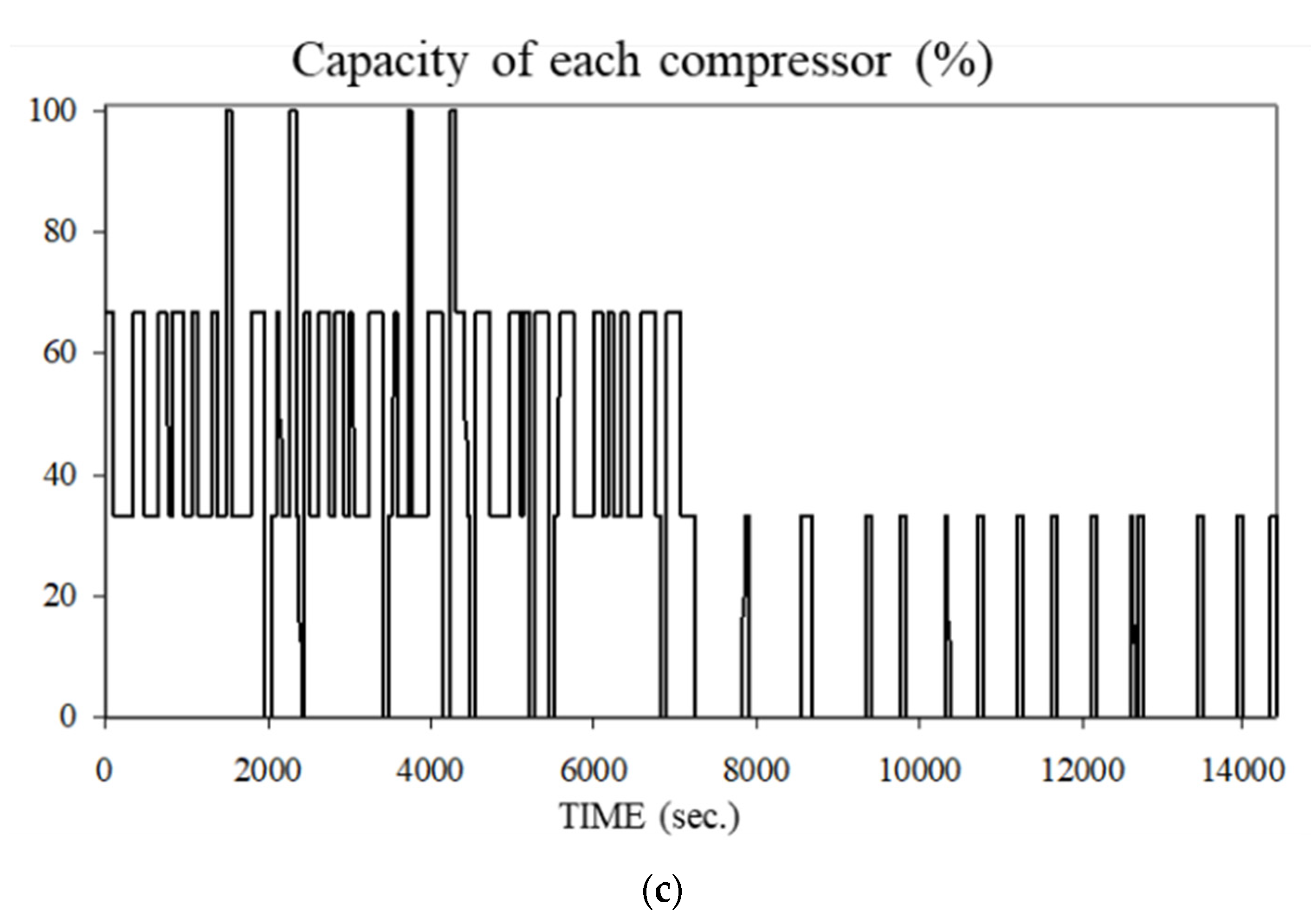
4.4. Analysis of the Solution
The optimal distribution of power, in other words, when the power of the compressors is (50, 20, 30), is shown in experiment 18 of
Table 1. The changes in air temperature in each display over four hours of simulation with HMPC controller acting on the process are shown in
Figure 9a. As from around thirty minutes, the three temperatures are stabilized and stayed at the desired interval between
and
over the first two hours of daytime operation. Then, a night-time mode starts (resumed with the use of the night covers). This ambient change introduces some small fluctuations and afterwards, the temperatures are also maintained within the desired range. In addition, it is important to point out that no synchronization of the temperatures in the display occurred, which is otherwise notable with the traditional control.
Figure 9b shows that the evolution of
Psuc, after the initial period, is maintained between a minimum of bar 1.1 and a maximum of bar 1.7 with minimal fluctuations. Following the change to the night-time mode of operation, after a few minutes during which it is below the minimum value, it stays within the new specifications but with broader fluctuations. Finally,
Figure 9c shows the on/off states of the compressors. The first compressor is stopped over the first two hours on only one occasion, and when turned on again the second compressor also starts up again. It is never necessary to contribute more than 70% of the installed power. Most notable of all is the night-time operation, with long periods of the first compressor turned off, which is the only one needed to maintain the controlled parameters (air temperatures in the three displays and suction pressure) within the desired range.
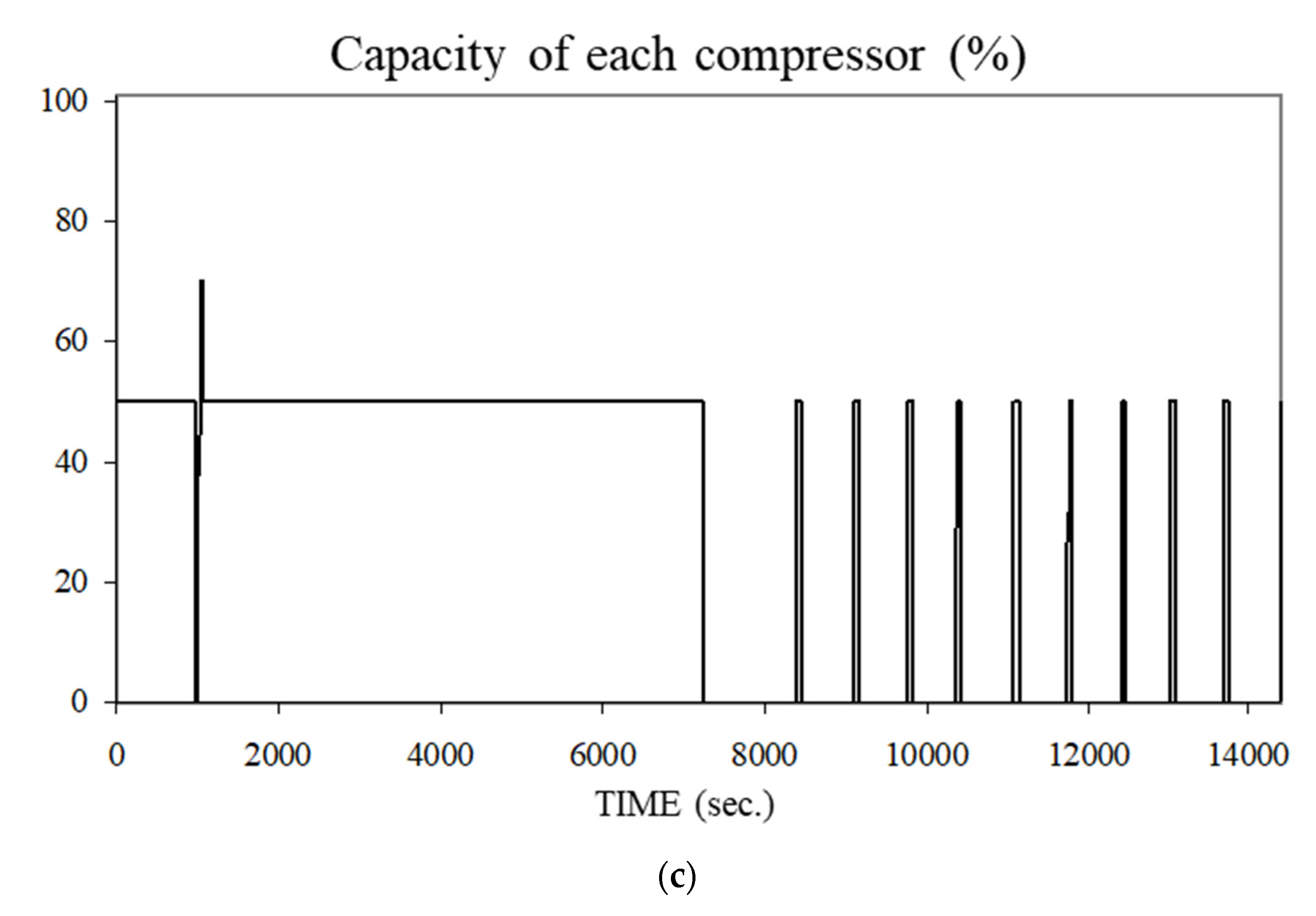
Figure 10 shows similar graphs to those in
Figure 9, but with a non-acceptable distribution of power, according to the global desirability function, in order to compare the evolution of the system and its dependence on the rack structure of the compressors (
Figure 8). One case (20, 80, 0), in particular, was considered: experiment 4,
Table 1. There were many constraint violations of the air temperature in the three displays, shown in
Figure 10a, and also of suction pressure, as in
Figure 10b. In addition, the two compressors very frequently start up and stop, particularly over the two first hours of daytime operation. Behaviour was acceptable over the following two hours. Globally, when
Figure 9 is compared, the poor performance of the rack configuration is evident in relation to system controllability.
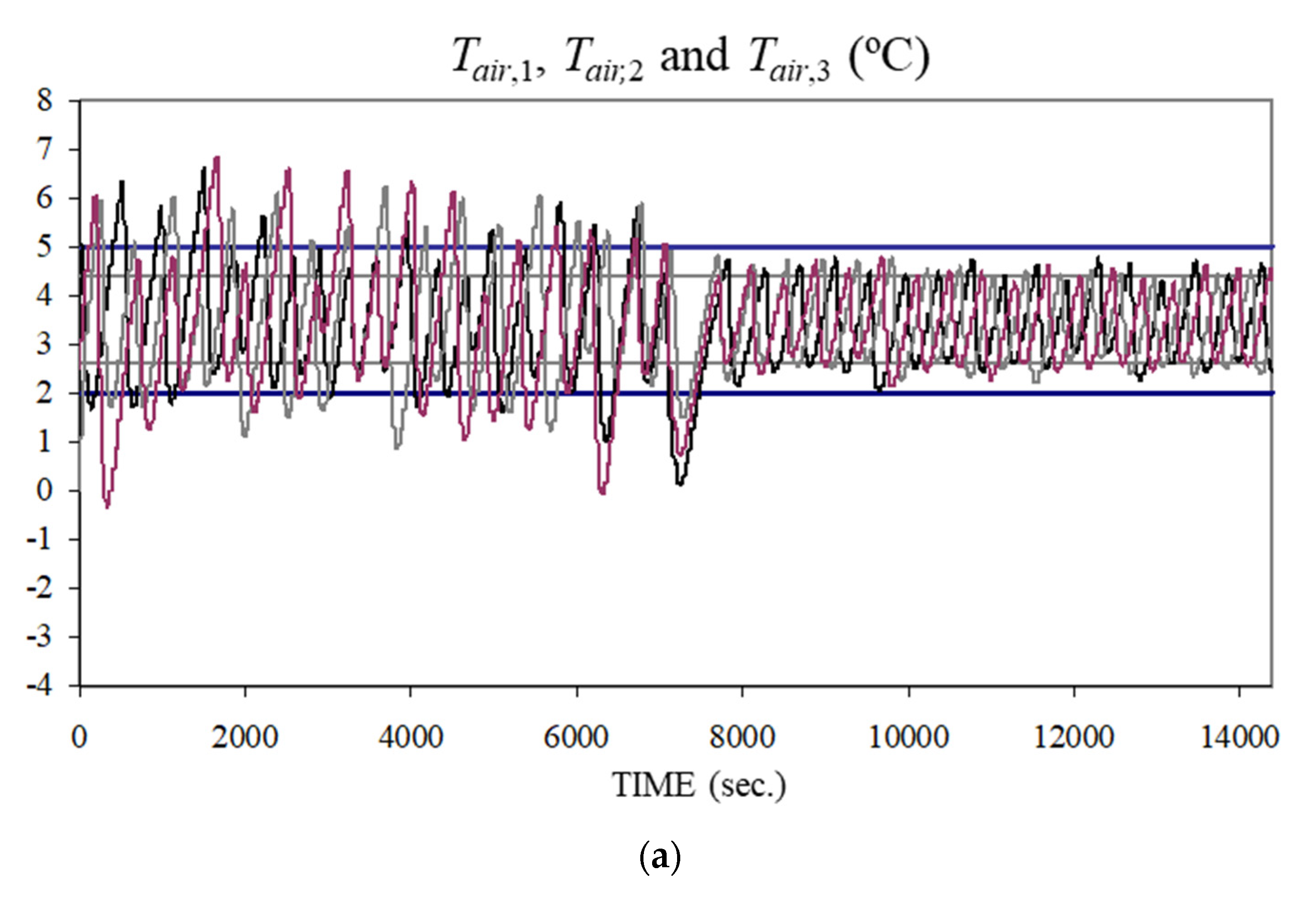
Experiment 15, the results of which are in
Table 1, has a configuration of three compressors of equal power, which could be considered “a priori” as a choice based on symmetry that reveals poor knowledge of a configuration based on system controllability. Its performance is shown in
Figure 11. It is clear that the optimal configuration,
Figure 9, has fewer constraint violations above all in the first two hours, both in the display temperatures,
Figure 11a, and in suction pressure,
Figure 11b. The effect is less in the two hours of night-time operation. The three compressors start and stop very frequently during the day, without achieving greater control over the system, as may be seen in
Figure 11c. Behaviour is more similar to the optimal configuration in
Figure 9c during the last two hours before the night-time period, but with 14 starts, as opposed to 9 in the optimum case.
5. Discussion
The discussion of the results shown in this work can be summarized in two points. First, a piece of new evidence about the increase of controllability and energy reduction when the process configuration and its control system are considered at the same time during the design phase is provided. Second, the use of surrogate linear models in the coefficients is feasible in computational experiments with complex models. Although there are not experimental errors, the least squares fit minimizes the distance between the surrogate model and the computational (complex or rigorous) model.
The advantages of the procedure are derived of the information provided by this distance. For a fixed number, N, of experiments to be performed, this distance allows one to explore the experimental domain to obtain a D-optimal design for the surrogate model. That is, the set of compressor configurations that leads to the most accurate estimation of the coefficients of the surrogate model. Increasing N provides a sequence of D-optimal designs. With each of them, the maximum loss function used in the fitting is evaluated throughout the experimental domain (criterion G). Thus, before starting the computational experiment, the researcher decides how many configurations and the structure of each of them will be used to obtain the surrogate model that best describes the performance control indices in the experimental domain. Then, the configuration in which the optimum is reached will be searched. This is a very flexible approach which, in addition, allows one to detect non-adequate surrogate models and increase its complexity sequentially.
Comparatively, if the optimal configuration of the compressors is sought through a computational experiment and a surrogate model based on machine learning, there is no formal relationship between the training set of experiments to be done and the loss function used in the fitting. As a result, it is not possible to estimate the number of experiments needed or their distribution in the experimental domain. This can lead to experimental overexertion and/or a higher probability of obtaining suboptimal solutions.
6. Conclusions
The research described in the paper shows that the Response Surface Methodology can be applied in computational experiments even though there is no random variability in the modelled response. This absence of variability is the fundamental and distinctive feature of computational experiments.
It is shown that it is sufficient to consider the metric character of the fit by means of least squares of the surrogate function. As consequence, an experimental design coupled with the desirability function has given us the tools to solve the problem of how to calculate the most efficient integrated design of a supermarket refrigeration system.
A mixture D-optimal design is a suitable option capable of modelling constraints that relate to the number of compressors and their capacity with the controllability indices.
With this approach, it was only necessary to make 16 computational experiments of the experimental domain consisting of 43 points to find the optimal number and capacity of the compressors.
Moreover, the controllability indices (day/night) have been improved: (1) the oscillations of suction pressure and air temperatures have decreased substantially; (2) all controlled variables are within their ranges; (3) during the day, only one compressor is enough (it is always on) (4) during the night, one compressor is sufficient with only 20 % of capacity, thus decreasing the power consumption.
In this work, a polynomial expansion of the design variables has been used to linearly model the integrated design. Its future development will be to extend this methodology to cases in which the nonlinearity of integrated design requires a surrogate model with more complex dependence on design variables. The core idea is to augment/replace the vector design variables with additional variables, which are transformations of them, for example: piecewise polynomials, multidimensional splines, gaussian radial basis functions, wavelet basis, or local regression.


