An Algorithm for Generating a Diverse Set of Multi-Modal Journeys

Abstract

A direct way of reducing the number of cars on the road is to dissuade individuals from exclusively using their car and instead integrate public transport into their daily routine. Planning multi-modal journeys is a complex task for which individuals often rely on decision support tools. However, offering individuals different journey options represents a significant algorithmic challenge. The failure to provide users with a set of journey options that differ considerably from one another in terms of the modes of transport employed is currently preventing the widespread uptake of multi-modal journey planning among the general public. In this paper, we introduce a dynamic programming algorithm that remedies this situation by modeling different transport networks as a graph that is then pruned by various graph-reduction pre-processing techniques. This approach enables us to offer a diverse set of efficient multi-modal solutions to users almost instantaneously. A computational study on three datasets corresponding to various real-world mobility networks with up to 30,000 vertices and 596,000 arcs demonstrates the effectiveness of the proposed algorithm.

1. Introduction

In recent years, a growing environmental consciousness and changing attitudes toward urban planning have led national governments and local authorities to encourage individuals to change their mobility habits. Instead of driving straight to their destination with their own private vehicle, individuals are encouraged to combine different modes of transport. Ultimately, this leads to fewer cars on the road and thus less greenhouse gases being released into the atmosphere. Fewer vehicles in city centers also relieves noisy congestion, making those spaces more liveable for residents and more attractive to visitors. More people using public transport also increases the revenue of those systems, enabling them to remain cost-effective for users while also providing the financial resources necessary for maintenance and expansion.

Multi-modal journey planning involves finding a path that combines different modes of transport to reach a destination location. Planning such journeys is often challenging due to the inherent complexity of linking together different journey legs [1]. One crucial constraining factor is that people must be given sufficient time to complete the transfer between different modes of transport. This is especially challenging when combining modes of transport that are always available, such as walking or car travel, with timetabled transport, such as trains or buses. The latter are not flexible modes of transport that are available on demand, but instead operate in accordance with predefined timetables.

Given the complexity involved in planning multi-modal journeys, many individuals rely on algorithmic decision support to optimize their routes. The underlying optimization algorithm should be sufficiently general to meet the demanding expectations of its users. Moreover, the algorithm should return solutions quickly enough to allow for (near) real-time usage of a journey-planning service. In addition to near-instantaneous responsiveness, the optimization algorithm we introduce in this paper also incorporates two additional crucial aspects:

• Inclusion of car travel Multi-modal journey planning combines different timetabled modes of (public) transport with unrestricted forms of mobility. In practice, car travel often remains an essential part of multi-modal journeys when, for example, the nearest public transport station is located too far away to reach on foot. The model proposed in this paper includes various ways of incorporating car travel to cover part of the journey.
• Solution diversity It is often not possible for users to express all of their preferences and restrictions. This may result from the restrictiveness of the journey planning system, which prevents users from inputting specific requirements. However, users prefer to have sufficiently unique options available to them so that they can select the one that best matches their preferences and restrictions. The algorithm introduced in this paper is therefore designed to return a set of diverse solutions rather than a single solution.

1.1. Multi-Modal Journey Planning

There have been a number of important contributions with respect to route and journey planning over the last twenty years. In road networks, shortest paths can be found in graphs consisting of millions of vertices and arcs in only a few milliseconds thanks to sophisticated algorithms that combine extensive pre-processing with intelligent search [2,3].

Journey planning problems that involve public transport are typically modeled using either time-expanded or time-dependent models. In a time-expanded model, there is a vertex for each event in the timetable. There are arcs between vertices representing events associated with the same trip as well as between vertices belonging to the same stop. Time-dependent models are generally smaller and consist of one vertex for each stop. Arcs between vertices (stops) are characterized by travel time functions that map departure times to arrival times. Several extensions and variations of these two basic models have been proposed, for example to handle fast updates of timetable-related data in case of delays [4].

Finding journeys in public transport networks is complicated by the fact that transfers, typically performed in a secondary network, also need to be included in solutions. Early methods for journey planning in public transport networks were restricted to transfers on foot between public transport stops [5]. Noteworthy early approaches to journey planning include round-based public transit optimized routing, the connection scan algorithm and trip-based public transit routing [6,7,8]. Common to these methods is the assumption that the graph used to model the transfer network is transitively closed: if transfers from location a to b and from location b to c are possible, then a transfer from location a to c should also be possible. For real-world public transport networks, this assumption can lead to very large transfer networks. Therefore, these three algorithms include additional restrictions that forbid lengthy transfers, based on the assumption that long transfers are rarely part of optimized journeys and are usually not preferred by users. These additional restrictions considerably reduce the number of edges in the transfer network.

More recently, research efforts have shifted toward solving what is the true multi-modal journey planning problem: combining public transport with a general unrestricted mode of transport. This unrestricted transfer network generalizes transitively-closed transfer networks to allow fully fledged routing in very large road or pedestrian networks. Baum et al. [9] achieved this by using a pre-processing technique that computes a small number of so-called transfer shortcuts that enable the discovery of optimal solutions. Falek et al. [10] employed a different pre-processing step in which the multi-modal network is partitioned. By using pre-computed shortest paths between the partitions in a bi-directional Dijkstra algorithm, solutions are found in short computation times. Potthoff and Sauer [11] solved a journey planning problem with transfers permitted between all modes of transport while optimizing for three objectives: arrival time, number of public transport trips used and time spent on transfers. They proposed an algorithm based on trip-based public transit routing [8] that eliminates the need to explicitly represent the Pareto set of non-dominated solutions.

Car travel in multi-modal journeys is often heavily restricted in existing approaches in order to limit the number of possible solutions and reduce computation time. For example, Delling et al. [12] only allowed car travel at either the beginning or end of a journey. As a result, journeys that employ car travel as an intermediary link between two modes of transport are not considered. Bast et al. [13] defined specific combinations of modes of transport to be feasible: (i) only car travel, (ii) public transport and walking but no car travel and (iii) mostly public transport, little walking and little car travel. They argued that journeys that do not conform to one of these three forms would always be disregarded by users and therefore may be safely discarded during optimization.

1.2. Solution Diversity

Users of route planning services typically prefer to have multiple options for reaching their destination [14]. This enables them to select the route that best matches their constraints and preferences that have not been configured in the route planning system. Moreover, it provides users with alternative options in case their preferred choice becomes unavailable due to unforeseen events. In the context of multi-modal journey planning, alternative solutions are therefore only meaningful if they differ in terms of the modes of transport they combine. Solutions that feature the same modes of transport and only differ in objective value will not be perceived as truly diverse.

Alternative paths have traditionally been computed using two general approaches: finding k shortest paths or finding disjoint paths. Algorithms designed to find k shortest paths do not guarantee that the different solutions are diverse [14]. Solutions are typically only different with respect to a few edges compared to the optimal solution, often introducing (small) detours. This makes these alternative solutions unattractive for users in the context of journey planning. Liu et al. [15] addressed the k shortest paths problem with solution diversity. The goal is to find k paths for which the similarity between any pair of paths lies below a threshold defined by the user. The objective is to minimize the total length of all k paths. Meanwhile, computing disjoint paths involves generating routes that share a maximum number of edges. Regardless of whether one employs a k shortest paths or a disjoint paths approach, the problem is computationally very challenging and cannot currently be addressed in the context of real-world road and public transport networks.

Other approaches to finding alternative paths have been explored over the years. The method proposed by Abraham et al. [16] uses intermediate destinations to find a series of path segments that can then be combined into a single journey to the destination. Bader et al. [17] used the concept of an alternative graph to encode many alternative paths in a compact manner. Kontogiannis et al. [14] extended this concept to find time-dependent shortest paths.

Delling and Wagner [18] proposed a multi-objective approach to generate a set of non-dominated paths in road networks. Their computational study demonstrated that such paths can only be found for relatively small networks. Multi-modal journey planning is also often modeled as a multi-objective problem that naturally leads to a set of solutions instead of a single solution. While the non-dominated solutions are guaranteed to differ in terms of objective function, there is no guarantee that their paths are truly diverse. To overcome this issue, we take diversity to refer to variety in terms of the modes of transport used to reach a destination.

1.3. Contributions

The present paper introduces an optimization algorithm for generating journeys from an origin to a destination location in a large-scale multi-modal network. A user query is characterized by an earliest possible departure time and a latest possible arrival time. The goal is to find journeys that are optimized with respect to three objectives: (i) arrival time, (ii) number of transfers and (iii) diversity in terms of the modes of transport used. A journey is considered feasible if it respects the aforementioned user query’s characteristics and combines different modes of transport in a feasible way, that is, by ensuring there is sufficient time for any transfers required. Depending on the network topology and the specific user query, the number of feasible journeys may vary considerably. For this reason, there is no constraint on the number of journeys to be returned by the algorithm. The problem is modeled as a multi-criteria shortest path problem in a directed graph that represents the multi-modal network [19]. Several graph pre-processing techniques reduce the size of the graph and improve algorithm run times.

The remainder of this paper is organized as follows. Section 2 details the proposed multi-modal journey planning model. Section 3 describes the search algorithm as well as the pre-processing techniques we propose to reduce the size of the graph. Section 4 evaluates the performance of our approach on multiple real-world mobility networks. Finally, Section 5 concludes the paper and identifies directions for future research.

2. Problem Model

This paper employs a graph-based model of the multi-modal journey planning problem. Let $G=(V,A)$ be a graph where $V=\{1,...,|V\left|\right\}$ is the set of vertices and $A=\{1,...,|A\left|\right\}$ is the set of arcs. Each vertex represents a physical location associated with a mode of transport, for example a platform in a train station or a parking location used for park-and-ride. Arcs between vertices represent the ability to travel between two locations. An arc $a\in A$ is characterized by its tail and head vertices $t\left(a\right)$ and $h\left(a\right)$, respectively. Note that the tail and head vertices must be different for an arc ($t\left(a\right)\ne h\left(a\right)$). It is possible for multiple arcs to connect the same pair of vertices when a user can travel between these two locations using different modes of transport.

We consider always-accessible modes of transport such as walking, cycling or driving as well as timetabled services such as train, metro or bus. The set of arcs $A^1\subseteq A$ is associated with modes that are always accessible. An always-accessible arc $a\in A^1$ is characterized only by the duration required to travel from $t\left(a\right)$ to $h\left(a\right)$, which is denoted by $d\left(a\right)$.

The arcs in set $A^2\subseteq A$ are associated with timetabled services. A timetabled arc $a\in A^2$ represents a timetabled mode of transport characterized by a set of departure and arrival times from $t\left(a\right)$ to $h\left(a\right)$. Because of the timetable, a user may need to wait for the next departure time at vertex $t\left(a\right)$. The waiting time when arriving at time t at vertex $t\left(a\right)$ is computed by the function $w(t,a)$. If two or more instantiations of the same timetabled mode of transport travel from vertex $t\left(a\right)$ to vertex $h\left(a\right)$, their timetables are merged. This may occur when, for example, there are two bus lines that serve the same two consecutive stops. The resulting aggregated timetable is then used to compute the waiting time. Note that timetables are only merged for instantiations of the same mode of transport. What this means is that in our example involving bus lines, the timetable of a train traveling between the same two stops will not be included in the aggregated timetable as it corresponds to a different mode of transport.

The considered modes of transport are defined by the set M. The elements in this set refer to general modes of transport—such as car, train or bus—and not to specific instantiations of these modes such as specific trains or buses. Each arc $a\in A$ is associated with one mode $m\left(a\right)\in M$.

As car travel is a special mode of transport that we wish to emphasize, Figure 1 illustrates the different forms car travel may assume. Figure 1i corresponds to traveling the entire journey by car, while Figure 1ii–iv illustrate different combinations of car travel and other modes of transport. A car can be used to cover the journey’s first/last mile or to travel to a park-and-ride location that is close to the destination. For first-mile car travel (Figure 1ii), always-accessible arcs are added between the origin vertex and hubs located close to the origin. Hubs are vertices of the graph that represent highly interconnected locations. Similarly, for last-mile car travel (Figure 1iii), arcs are added between hubs close to the destination vertex and the destination vertex itself. To model driving to park-and-ride locations (Figure 1iv), always-accessible arcs are added between the origin vertex and vertices close the destination that represent park-and-ride locations. Each of these forms of car travel is considered a unique mode of transport, and will therefore be included separately in M. By doing so, a distinction is made between the different forms of car travel, allowing for greater solution diversity. Note that arcs representing these modes are added to G when a query is made as they connect query-dependent origin and destination vertices to existing vertices in G.

A user query requests feasible paths in G from an origin vertex $o\in V$ to a destination vertex $d\in V$. The query also specifies an earliest departure $t^{\mathrm{start}}$ and a latest arrival time $t^{\mathrm{end}}$. A path is defined as a sequence of n arcs $P=\{a_1,...,a_n\}$ with $a_k\in A,\forall k\in \{1,...,n\}$. Consecutive arcs are connected by a vertex such that $h\left(a_k\right)=t\left(a_{k+1}\right),\forall k\in \{1,...,n-1\}$. A path passes through any vertex at most once, such that $t\left(a_k\right)\ne t\left(a_k^{\prime }\right),\forall k,k^{\prime }\in \{1,...,n\},k\ne k^{\prime }$. Let $o\left(P\right)$ be the initial vertex of path P, which corresponds to vertex $t\left(a_1\right)$. Let $d\left(P\right)$ be the final vertex of path P, which corresponds to vertex $h\left(a_n\right)$. A complete path is one for which $o\left(P\right)=o$ and $d\left(P\right)=d$.

FIFO Violations

The first-in-first-out (FIFO) property guarantees that it is impossible to arrive at a destination earlier by postponing the journey’s departure time. Our method assumes that this property holds on arcs, meaning that vehicles never overtake each other between an arc’s tail and head vertices. For non-timetabled modes of transport, it is generally accepted that time-dependent travel times on arcs should respect the FIFO property [20]. For modes of transport that operate on a timetable, it is reasonable to assume that the timetable has been constructed in such a way that the FIFO property is respected between two consecutive stops. Note that this assumption forbids overtaking to take place en route between two consecutive stops, but still allows timetabled vehicles to overtake each other at a stop by scheduling additional waiting time between a vehicle’s arrival and departure to enable another vehicle to depart earlier from that same stop.

While FIFO violations on a single arc could theoretically occur for a timetabled mode of transport, we consider these events to be highly unlikely in practice. This situation would look something like the following. Imagine there are two buses traveling directly from stop A to stop B. The first bus leaves at 9:00 a.m. and arrives at 9:30 a.m., while the second bus leaves at 9:05 a.m. but arrives at 9:25 a.m. When determining the earliest departure time based on the aggregated timetable of these two buses, the algorithm will choose the first bus even though the second bus would actually lead to an earlier arrival time at B. In this unusual scenario, the algorithm will not generate a solution with the earliest possible arrival time at the final destination.

3. Routing Algorithm

This section introduces the algorithm that searches non-dominated paths in graph G with respect to the three criteria outlined in Section 1.3. A number of pre-processing techniques are also introduced to reduce the graph’s size and the algorithm’s run time, namely graph cutting, vertex merging, footpath arc pruning and arc restriction.

3.1. Search Algorithm

The proposed algorithm uses states to represent (partial) paths. A state ${\sigma }_P$ is defined to hold the following information concerning a path P:

$${\sigma }_P=\left(i,a,{\mathcal{J}}_i,{\mathcal{T}}_i,{\mathcal{M}}_i\right)$$

(1)

where i is the last vertex visited in path P and a is the arc used to reach this vertex, such that $h\left(a\right)=i$. Variable ${\mathcal{J}}_i$ is the time at which vertex i is reached, while ${\mathcal{T}}_i$ corresponds to the number of transfers made along the path. A transfer is counted each time a different mode of transport is employed in the sequence of the solution path. However, to avoid penalizing short transfers by foot, a threshold parameter $\pi$ is employed. What this means is that as long as the walking duration is less than $\pi$, it will not count as an additional transfer. For example, the walk itself when changing between two buses located very close to each other at a transport hub will not be counted if it does not take longer than $\pi$. Finally, ${\mathcal{M}}_i$ is the set of modes of transport used along the path. Journey time and number of transfers are widely employed objectives in the literature [6,21,22,23]. However, we introduce ${\mathcal{M}}_i$ as an additional variable in a state to enable differentiating between solutions that use different modes of transport, and can thus be considered diverse.

Algorithm 1 extends a state along each outgoing arc a of ${\sigma }_P\left(i\right)$ in G, thereby producing a new state in which the partial path is extended from the current node $t\left(a\right)$ (which equals ${\sigma }_P\left(i\right)$) to the next node $h\left(a\right)$. The variables in the states are updated as follows:

$$\begin{array}{cc}\hfill {\mathcal{J}}_{h\left(a\right)}& =\left\{\begin{array}{ccc}{\mathcal{J}}_{t\left(a\right)}+w({\mathcal{J}}_{t\left(a\right)},a)+d\left(a\right)\hfill & & \mathrm{if}a\mathrm{is}\mathrm{a}\mathrm{timetabled}\mathrm{arc}\hfill \\ {\mathcal{J}}_{t\left(a\right)}+d\left(a\right)\hfill & & \mathrm{otherwise}\hfill \end{array}\right.\hfill \end{array}$$

(2)

$$\begin{array}{cc}\hfill {\mathcal{T}}_{h\left(a\right)}& =\left\{\begin{array}{ccc}{\mathcal{T}}_{t\left(a\right)}\hfill & & \mathrm{if}a\mathrm{is}\mathrm{a}\mathrm{footpath}\mathrm{arc}\mathrm{and}d\left(a\right)\le \pi \hfill \\ {\mathcal{T}}_{t\left(a\right)}+1\hfill & & \mathrm{otherwise}\hfill \end{array}\right.\hfill \end{array}$$

(3)

$$\begin{array}{cc}\hfill {\mathcal{M}}_{h\left(a\right)}& ={\mathcal{M}}_{t\left(a\right)}\cup m\left(a\right)\hfill \end{array}$$

(4)

Note that ${\mathcal{M}}_i$ is implemented as a set containing only unique values corresponding to the modes of transport used in path P and will therefore not be updated if the path continues using the same mode of transport. If the partial path is extended with a timetabled arc, the earliest possible departure time at node $t\left(a\right)$ is always selected. A state is considered feasible if ${\mathcal{J}}_i$ is less than or equal to the user’s latest arrival time $t^{\mathrm{end}}$. States associated with paths that do not respect this condition are not extended.

Using the information stored in the states, we can determine conditions to define when one path dominates another, thereby allowing some states to be discarded. Consider two states ${\sigma }_P$ and ${\sigma }_P^{\prime }$ that have reached the same node i. State ${\sigma }_P$ dominates ${\sigma }_P^{\prime }$ when all of the following conditions hold with at least one strict inequality:

$$\begin{array}{cc}& {\mathcal{J}}_i\le {\mathcal{J}}_i^{\prime }\end{array}$$

(5)

$$\begin{array}{cc}& {\mathcal{T}}_i\le {\mathcal{T}}_i^{\prime }\end{array}$$

(6)

$$\begin{array}{cc}& {\mathcal{M}}_i\subseteq {\mathcal{M}}_i^{\prime }\end{array}$$

(7)

The algorithm iterates through all elements in a priority queue Q that prioritizes partial paths that have the earliest arrival time at the destination vertex. This arrival time is calculated by the path’s current time plus an estimation of the additional time required to reach the destination. More specifically, the priority cost is set to ${\sigma }_P\left({\mathcal{J}}_i\right)+\theta \left({\sigma }_P\left(i\right)\right)$, where ${\sigma }_P\left({\mathcal{J}}_i\right)$ is the time in the state associated with path P and $\theta \left({\sigma }_P\left(i\right)\right)$ is a lower bound on the estimated remaining time to destination. $\theta \left({\sigma }_P\left(i\right)\right)$ is calculated by dividing the distance determined by the haversine formula from the final vertex in path P to the destination vertex d by the maximum speed in the network. The function extend(${\sigma }_P,a$) extends state ${\sigma }_P$ along arc a and only returns a value if the new state is feasible. Whenever a new state is added to either the set of solutions $\mathcal{S}$ (line 7) or to the priority queue Q (line 12), dominated states are also removed from these collections.

Due to the various problem elements, it is not immediately clear how many (partial) paths can be dominated in each iteration of the algorithm or in total. To assess the algorithm’s time complexity, we therefore consider the worst case in which no paths are dominated. Let $\lambda$ denote the number of possible solutions. The necessary updates when extending a partial path (Equations (2)–(4)) are performed in constant time. Verifying the dominance conditions (Equations (5)–(7)) requires $\mathcal{O}\left(\right|M\left|\right)$ time due to Equation (7). In the worst case, we may have to compare each solution against all others every iteration to verify dominance, which requires $\mathcal{O}\left({\lambda }^2\right)$ dominance tests. This results in the algorithm exhibiting a worst-case time complexity of $\mathcal{O}\left({\lambda }^2\right|M\left|\right)$. The number of solutions is exponential in the number of vertices of the graph. More specifically, a bound on the number of solutions is defined as $\mathcal{O}\left(\lambda \right)={\sum }_{k=1}^{n}n!/(n-k)!$ with $n=\left|V\right|-2$. The worst-case time complexity depends on the number of modes, which means having fewer modes also improves algorithm performance. Note that if only arrival time and number of transfers are considered as objectives, the worst-case complexity is reduced to $\mathcal{O}\left({\lambda }^2\right)$ as all dominance criteria can be verified in constant time.

3.2. Graph Pre-Processing

The number of states explored by Algorithm 1 primarily depends on the size of graph G. Therefore, in an effort to reduce the number of states, and by extension the algorithm run time, four pre-processing techniques are applied to reduce the number of vertices and arcs in G. These techniques have been designed to exclude (partial) paths that users would avoid in practice, thereby not significantly affecting the quality of the returned solutions.

Algorithm 1  Search algorithm.

1: procedure  ShortestPath($o,d,t^{\mathrm{start}},t^{\mathrm{end}}$) 2:     $Q\leftarrow \left\{(o,\varnothing ,t^{\mathrm{start}},0,\varnothing )\right\}$ 3:     $\mathcal{S}\leftarrow \varnothing$ 4:     while Q is not empty do 5:         ${\sigma }_P\leftarrow$pop(Q) 6:         if ${\sigma }_P\left(i\right)$=d then 7:            $\mathcal{S}\leftarrow$add(${\sigma }_P$) 8:         else 9:            for all outgoing arc aof${\sigma }_P\left(i\right)$ do 10:                ${\sigma }_P^{\prime }\leftarrow$extend(${\sigma }_P,a$) 11:                if ${\sigma }_P^{\prime }$ is non-dominated then 12:                    $Q\leftarrow$add(${\sigma }_P^{\prime }$) 13:     return $\mathcal{S}$

3.2.1. Graph Cutting

Wagner et al. [24] used geometric containers that precompute, for each arc of the graph, whether or not it can be safely removed for a specific query. They considered different geometric containers, such as bounding boxes and ellipses, and concluded that bounding boxes perform consistently well. A rectangular bounding box parallel to a line of latitude and whose sides are in proportion with origin and destination locations would intuitively appear to be the logical choice given that it is used in the road network problem [21]. However, the nature of multi-modal journeys means that oftentimes one will have to pass through an important hub whose location may not lie on the direct path between the journey’s origin and destination. Therefore, a rectangular bounding box with sides of equal length, in other words a square, is employed here as a more appropriate alternative. The length of each side of the bounding box is computed as follows:

$$max(Dma{x}_{o,d}+\alpha ,Dma{x}_{o,d}\times \beta )$$

(8)

where $Dma{x}_{o,d}=max(Dlat(o,d),$$Dlon(o,d))$, and $Dlat(o,d)$ and $Dlon(o,d)$ are the latitudinal and longitudinal distances from the origin to the destination, respectively.

3.2.2. Vertex Merging

The number of vertices in G can grow considerably when combining multiple modes of transport. However, some vertices may represent nearby locations, such as different platforms in a train station. Merging these vertices into a single vertex reduces graph size and improves computational time.

A new graph is created in which some vertices from the original graph are merged together. First, all vertices are sorted in descending order based on their connectivity. This enables us to identify the Highest Connectivity Vertex (HCV). The HCV will correspond to a vertex in the new graph, thereby maintaining all of its incoming and outgoing arcs. When considering the current HCV, all of its outgoing footpath arcs are iterated over. For each footpath arc, its corresponding head vertex may be merged with the HCV only if the following three conditions hold: (i) it has not been processed before, (ii) the distance between the two vertices does not exceed a predefined threshold $\mathcal{R}$ and (iii) the two vertices are only connected by a footpath arc. The final condition avoids merging vertices connected together by another mode of transport, which implies they are relevant locations that should not be merged. After all of the footpath arcs associated with the HCV have been processed, the next HCV is selected from the ordered list. An internal transfer time $\varphi$ is used to model the time needed to travel between merged vertices. Note that if $\varphi \le \pi$, an internal transfer will not be counted towards the total number of transfers in the path.

3.2.3. Footpath arc Pruning

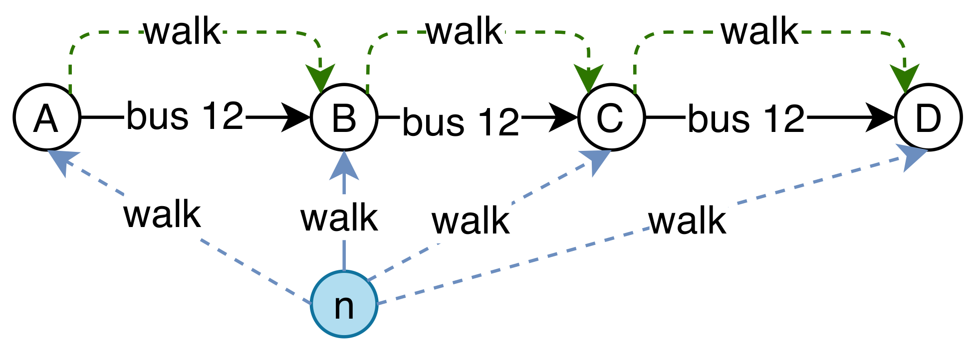
Another factor that considerably impacts the size of graph G is the number of footpath arcs. To reduce the number of such arcs, we first assume users are not willing to walk more than $\gamma$ kilometers. However, many of the remaining footpath arcs can be safely removed without significantly affecting solution quality. From a human perspective, when a user wishes to take a specific bus line, they will most likely walk to the nearest bus stop for that line and not a stop that is much further away. Similarly, when a user is at the bus stop waiting for a bus, we assume they will not walk to the next stop, even if it could save them time. Graph G is modified by removing specific footpath arcs when they are deemed inessential, that is, when it is unlikely they will ever be used in desirable solutions. This is realized by iterating over all vertices and enumerating for each vertex v all outgoing transportation alternatives (the so-called transport identifiers). Starting from vertex v and continuing to the nearest vertex by distance $v^{\prime }$, the footpath arc between v and $v^{\prime }$ is pruned if and only if there are no outgoing arcs in $v^{\prime }$ with transport identifiers that were unavailable at v.

Figure 2 shows an example in which vertex n has outgoing footpath arcs to all stops for bus 12, which have been labeled A, B, C and D. In this example, only the arc to the nearest stop will be kept (the solid blue arc), while all other outgoing arcs from n are removed (the dashed blue arcs). Similarly, all footpath arcs between bus stops of the same line, which are also connected by timetabled arcs for at least one bus line, are also removed (dashed green arcs).

3.2.4. Arc Restriction

The number of states to explore may be further limited by restricting the use of footpath arcs under specific circumstances. Figure 3 extends the example from Figure 2 and adds an arc between vertices C and G traversed by bus 14. In contrast to the previous example, the footpath arc from vertex n to vertex C must now be maintained so as to not ignore the connection to bus 14 offered at node C. However, traversing the footpath arc from vertex n to vertex B will also explore bus 12 and, therefore, it is unnecessary to explore bus 12 when traversing the footpath arc from vertex n to vertex C. To verify this condition, line 9 in Algorithm 1 is extended to determine which arcs may be extended based on those already in the path.

4. Computational Study

A series of computational experiments was conducted to quantify the performance of the algorithm detailed in Section 3.

4.1. Data and Experimental Setup

The General Transit Feed Specification (GTFS) is the standard for publishing public transport schedules. GTFS information from three different networks was selected: Belgium, London and New York City [25]. These networks vary significantly in terms of size and therefore provide a useful means of examining how the algorithm scales.

Table 1. Networks employed in the experiments.

Network	Operator Information				Graph Information
	Stops	Routes	Trips	Departure Events	Vertices	Timetabled Arcs	Footpath Arcs
London	379	255	53,809	1,246,770	379	844	5195
New York City	991	210	19,842	550,495	991	1142	31,627
Belgium	30,886	7208	214,447	6,942,668	30,886	37,786	558,953

details the number of stops, routes, trips, departure events and the size of the resulting graph before any pre-processing takes place. Two timetabled mobility operators were employed in the Belgian network: NMBS, which operates rail services, and De Lijn, which operates tram and bus services. Transport For London was employed for the London network and MTA New York City Transit for New York City, both of which cover the tram, rail, bus and metro services in their respective cities.

Hubs in each network used for car travel were identified by first sorting the vertices in G based on the number of outgoing and incoming arcs, in descending order, and then marking the first 50 vertices that are located at least two kilometers apart as hubs. No time limit was imposed for the experiments, which means Algorithm 1 stops when the priority queue is empty. Therefore, the final solutions are dominant considering the three criteria detailed in Section 3.1: journey time, number of transfers and modes of transport used. Unless mentioned otherwise, the following algorithm parameter settings were used: graph cutting $\alpha =5$ km and $\beta =150\%$, vertex merging distance $\mathcal{R}=0.1$ km, footpath arc pruning $\gamma =2.5$ km, internal transfer time $\varphi =2$ minutes and transfer threshold $\pi =15$ minutes. 1000 random queries were executed for each network, with the reported values corresponding to the average of these queries. The origin and destination vertices for these queries were chosen randomly from the set of vertices V in a uniform manner. All experiments were conducted on a Dell Poweredge T620, 2x Intel Xeon E5-2670 with 128GB RAM running a Linux-based operating system.

4.2. Vertex Merging

The first experiment investigated the impact of varying the merging distance parameter, $\mathcal{R}$.

Table 2. Performance metrics for vertex merging with different parameter settings.

$\mathcal{R}$	London			New York City			Belgium
	Vertices	Run Time	Quality	Vertices	Run Time	Quality	Vertices	Run Time	Quality
0 m	379	10 ± 6	100.0	991	25 ± 10	100.0	30,886	833 ± 418	100.0
100 m	372	11 ± 5	98.3	473	29 ± 11	96.7	16,529	769 ± 367	93.0
250 m	372	11 ± 5	98.3	473	30 ± 10	96.7	16,529	784 ± 370	93.0
500 m	357	9 ± 4	94.7	429	19 ± 7	93.3	14,817	707 ± 308	88.8
750 m	340	9 ± 6	91.9	384	14 ± 4	90.9	12,806	550 ± 234	87.9
1000 m	316	7 ± 3	87.0	332	12 ± 10	88.7	10,162	497 ± 211	88.1

presents results for different values of $\mathcal{R}$. For each network, the number of vertices, average run time in milliseconds, standard deviation of the run time and a quality metric are reported. The quality metric measures the percentage of identical dominant solutions against those obtained when no vertices are merged [26]. This metric is important as it identifies a possible loss in quality when employing this pre-processing technique.

Depending on the value of the distance merging parameter, vertex merging reduced the number of vertices by 46.5% to 67.1% in Belgium and 52.3% to 66.5% in New York City, but only 1.8% to 16.6% in London. Given that the London network is highly interconnected, only a small number of the vertices satisfy the vertex merging conditions. The algorithm’s run times for the London and New York City networks were very low, even without vertex merging. For the largest network, the Belgium network, vertex merging resulted in a speed-up ranging from 7.7% to 40.3%.

4.3. Algorithm Performance

We now investigate the impact of applying all four techniques from Section 3 to the networks.

Table 3. Impact of graph pre-processing.

	London			New York City			Belgium
	Arcs	Run Time	Quality	Arcs	Run Time	Quality	Arcs	Run Time	Quality
No pre-processing	6039	10 ± 6	100.0	32,769	25 ± 10	100.0	596,739	833 ± 418	100.0
Graph cutting	6039	6 ± 6	97.7	32,769	17 ± 12	99.4	596,739	392 ± 313	95.7
Vertex merging	5784	6 ± 4	96.2	11,257	16 ± 10	98.2	199,470	362 ± 301	90.4
Arc pruning	3611	5 ± 3	95.4	5945	12 ± 7	97.8	117,523	264 ± 212	86.7
Arc restriction	3611	5 ± 3	95.4	5948	12 ± 8	97.8	117,523	260 ± 209	86.7

reports the number of arcs in G, average run time in milliseconds, standard deviation of run time, and the aforementioned quality metric for each network when using the four pre-processing techniques. Note that graph cutting, vertex merging, arc pruning and arc restriction are applied incrementally, with their order of implementation corresponding to the degree to which they alter the graph.

The results demonstrate how the algorithm’s execution time without pre-processing techniques is, on average, less than a second. Each of the pre-processing techniques further decreases the execution time. However, for both the London and New York City networks it is difficult to infer the impact of the pre-processing techniques because the initial execution time values for the base algorithm were already very short. On the other hand, the Belgium network demonstrated a 68.8% speed-up when applying the four pre-processing techniques, with only a 13.3% decrease concerning the quality of dominant solutions. However, if only graph cutting is employed then a 52.9% speed-up can be obtained with an impact of only 4.3% on solution quality. When examining the number of arcs, the pre-processing techniques greatly reduced the size of the graph, thereby positively affecting algorithm run time. The reduction of the number of arcs after applying graph cutting, vertex merging and arc pruning was 86.3% in Belgium, 46.7% in London and 84.8% in New York City.

4.4. Diversity Analysis

As discussed in Section 3.1, in addition to journey time and number of transfers, the used mode of transport ${\mathcal{M}}_i$ is also taken into account as a dominance criterion. While this increases the number of non-dominated states, it enables us to differentiate between solutions that employ diverse modes of transport to reach the destination. The experiment discussed in this subsection analyzed the impact of including ${\mathcal{M}}_i$ as a dominance criterion on algorithm performance and solution diversity.

Table 4. Diversity analysis.

Dominance Criteria	Run Time	# Sols.	Avg. Sim${}_1$
London
${\mathcal{J}}_i,{\mathcal{T}}_i\mathrm{and}{\mathcal{M}}_i$	10 ± 6	3.03	0.10
${\mathcal{J}}_i\mathrm{and}{\mathcal{T}}_i$	7 ± 1	1.12	0.03
${\mathcal{J}}_i$	4 ± 0	1.00	-
New York City
${\mathcal{J}}_i,{\mathcal{T}}_i\mathrm{and}{\mathcal{M}}_i$	25 ± 10	2.92	0.09
${\mathcal{J}}_i\mathrm{and}{\mathcal{T}}_i$	27 ± 7	1.15	0.07
${\mathcal{J}}_i$	15 ± 3	1.00	-
Belgium
${\mathcal{J}}_i,{\mathcal{T}}_i\mathrm{and}{\mathcal{M}}_i$	833 ± 418	5.38	0.19
${\mathcal{J}}_i\mathrm{and}{\mathcal{T}}_i$	538 ± 188	1.18	0.41
${\mathcal{J}}_i$	256 ± 110	1.00	-

compares the performance of three configuration settings of the algorithm: (i) using all three dominance criteria, (ii) using journey time ${\mathcal{J}}_i$ and number of transfers ${\mathcal{T}}_i$ as dominance criteria, and (iii) using journey time ${\mathcal{J}}_i$ as the only dominance criterion, essentially solving a shortest path problem. Solution diversity is quantified by computing the similarity between journeys returned by the algorithm. Therefore, in addition to the average run time in milliseconds, standard deviation of run time and the average number of solutions found (# Sols.), a similarity metric Sim${}_1$ is also reported. This metric is the weighted Jaccard distance and ranges from 0 to 1, reflecting how many arcs are shared between solutions [15]. A value of 0 indicates that journeys share no arcs whereas a value of 1 indicates that all journeys are identical. The weighted Jaccard distance is computed by Equation (9), where $S_P$ is the set of arcs in path P and $L\left(S_P\right)$ is the length of the arcs in set $S_P$. Note that when only journey time ${\mathcal{J}}_i$ is considered, the similarity metric cannot be computed as only one solution is returned.

$${\mathrm{Sim}}_1(S_{P_i},S_{P_j})=\frac{L(S_{P_i}\cap S_{P_j})}{L(S_{P_i}\cup S_{P_j})}$$

(9)

The results demonstrate that the number of solutions is clearly affected by the number of dominance criteria included. The setting that resulted in the highest number of solutions is when all three criteria are included. However, this also negatively impacts the required computation time. When comparing the single-objective setting against including all three dominance criteria, the required run time doubled or even almost tripled depending on the network. Finally, the results demonstrate that when including ${\mathcal{M}}_i$, journey similarity is impacted, however, not always positively. For the Belgium network, the returned solutions are very diverse, whereas the journeys returned for the London and New York City networks were more similar. Note that an exact comparison between the two multi-objective settings is complicated as the number of solutions also impacts journey similarity.

5. Conclusions and Future Work

As modern cities are evolving, point-to-point car travel must be replaced with more sustainable and environmentally friendly options. Multi-modal journey planning helps individuals circumvent the challenge of combining several modes of transport, providing them with multiple alternatives that meet their travel requirements. This paper introduced a routing algorithm that enables a diverse set of solutions to be offered to users, thereby delegating a part of the decision making process to them.

Our contribution is threefold in nature. First, in addition to commonly considered modes of transport, park-and-ride locations were included in the graph to increase user convenience and flexibility. Second, the modes of transport used in a solution was introduced as a dominance criterion to provide a more diverse set of solutions. Third, we proposed four pre-processing techniques to improve the performance of the search algorithm: graph cutting, vertex merging, footpath arc pruning and arc restriction. Providing near-instant solutions helps improve user experience and is critical for real-world applications. By reducing the size of the graph, the algorithm’s run times are decreased, with only a small impact on quality. These techniques are simple to apply and modify. It is important to note that the balance between algorithm run time and solution quality may differ among different real-world applications and therefore there can be no one-size-fits-all approach.

Future research on multi-modal journey planning concerns four important directions. First, the proposed approach may be applied to other multi-modal settings, which would enable a comparison with alternative state-of-the-art approaches. Second, additional pre-processing techniques may continue to improve performance without significantly affecting solution quality—for example, arc pruning depending on user preferences and restrictions. A theoretical analysis of the impact of the pre-processing techniques on the algorithm’s run time complexity can support the reported computational results. Third, integrating network disruption or real-time traffic information represents an interesting challenge that requires additional efficient pre-processing. Finally, the possibility of obtaining more data concerning how users choose between different journeys may help understand what solution diversity actually means and how it could be better quantified. What this could entail is extending the model with more subjective parameters related to how users perceive the effort associated with using specific modes of transport.

References

- Rehrl, K.; Bruntsch, S.; Mentz, H.J. Assisting multimodal travelers: Design and prototypical implementation of a personal travel companion. IEEE Trans. Intell. Transp. Syst. 2007, 8, 31–42. [Google Scholar] [CrossRef]
- Bast, H.; Funke, S.; Sanders, P.; Schultes, D. Fast routing in road networks with transit nodes. Science 2007, 316, 566. [Google Scholar] [CrossRef] [PubMed]
- Geisberger, R.; Sanders, P.; Schultes, D.; Delling, D. Contraction Hierarchies: Faster and Simpler Hierarchical Routing in Road Networks. In Proceedings of the International Workshop on Experimental and Efficient Algorithms, Provincetown, MA, USA, 30 May–1 June 2008; pp. 319–333. [Google Scholar]
- Giannakopoulou, K.; Paraskevopoulos, A.; Zaroliagis, C. Multimodal dynamic journey-planning. Algorithms 2019, 12, 213. [Google Scholar] [CrossRef]
- Pyrga, E.; Schulz, F.; Wagner, D.; Zaroliagis, C. Efficient models for timetable information in public transportation systems. J. Exp. Algorithmics 2007, 12, 1–39. [Google Scholar] [CrossRef]
- Delling, D.; Pajor, T.; Werneck, R.F. Round-Based Public Transit Routing. Transp. Sci. 2015, 49, 591–604. [Google Scholar] [CrossRef]
- Dibbelt, J.; Pajor, T.; Strasser, B.; Wagner, D. Connection scan algorithm. J. Exp. Algorithmics JEA 2018, 23, 1–56. [Google Scholar] [CrossRef]
- Witt, S. Trip-based public transit routing. In Algorithms-ESA 2015; Springer: Berlin/Heidelberg, Germany, 2015; pp. 1025–1036. [Google Scholar]
- Baum, M.; Buchhold, V.; Sauer, J.; Wagner, D.; Zündorf, T. UnLimited TRAnsfers for Multi-Modal Route Planning: An Efficient Solution. In Proceedings of the 27th Annual European Symposium on Algorithms (ESA 2019), Munich/Garching, Germany, 9–11 September 2019; Bender, M.A., Svensson, O., Herman, G., Eds.; Leibniz International Proceedings in Informatics (LIPIcs); Schloss Dagstuhl–Leibniz-Zentrum fuer Informatik: Dagstuhl, Germany, 2019; Volume 144, pp. 14:1–14:16. [Google Scholar] [CrossRef]
- Falek, A.M.; Pelsser, C.; Julien, S.; Theoleyre, F. Muse: Multimodal separators for efficient route planning in transportation networks. Transp. Sci. 2022, 56, 436–459. [Google Scholar] [CrossRef]
- Potthoff, M.; Sauer, J. Fast Multimodal Journey Planning for Three Criteria. In Proceedings of the 2022 Symposium on Algorithm Engineering and Experiments (ALENEX), Alexandria, VA, USA, 9–10 January 2022; pp. 145–157. [Google Scholar]
- Delling, D.; Pajor, T.; Wagner, D. Accelerating multi-modal route planning by access-nodes. In Proceedings of the 17th Annual European Symposium, Copenhagen, Denmark, 7–9 September 2009; pp. 587–598. [Google Scholar] [CrossRef]
- Bast, H.; Brodesser, M.; Storandt, S. Result diversity for multi-modal route planning. In Proceedings of the ATMOS-13th Workshop on Algorithmic Approaches for Transportation Modelling, Optimization, and Systems, Sophia Antipolis, France, 5 September 2013; pp. 123–136. [Google Scholar] [CrossRef]
- Kontogiannis, S.; Paraskevopoulos, A.; Zaroliagis, C. Time-Dependent Alternative Route Planning: Theory and Practice. Algorithms 2021, 14, 220. [Google Scholar] [CrossRef]
- Liu, H.; Jin, C.; Yang, B.; Zhou, A. Finding top-k shortest paths with diversity. IEEE Trans. Knowl. Data Eng. 2017, 30, 488–502. [Google Scholar] [CrossRef]
- Abraham, I.; Delling, D.; Goldberg, A.V.; Werneck, R.F. Alternative routes in road networks. J. Exp. Algorithmics 2013, 18, 23–34. [Google Scholar] [CrossRef]
- Bader, R.; Dees, J.; Geisberger, R.; Sanders, P. Alternative route graphs in road networks. In Proceedings of the International Conference on Theory and Practice of Algorithms in (Computer) Systems, Rome, Italy, 18–20 April 2011; pp. 21–32. [Google Scholar]
- Delling, D.; Wagner, D. Pareto paths with SHARC. In Proceedings of the International Symposium on Experimental Algorithms, Dortmund, Germany, 4–6 June 2009; pp. 125–136. [Google Scholar]
- Modesti, P.; Sciomachen, A. A utility measure for finding multiobjective shortest paths in urban multimodal transportation networks. Eur. J. Oper. Res. 1998, 111, 495–508. [Google Scholar] [CrossRef]
- Ichoua, S.; Gendreau, M.; Potvin, J.Y. Vehicle dispatching with time-dependent travel times. Eur. J. Oper. Res. 2003, 144, 379–396. [Google Scholar] [CrossRef]
- Bast, H.; Delling, D.; Goldberg, A.; Müller-Hannemann, M.; Pajor, T.; Sanders, P.; Wagner, D.; Werneck, R.F. Route Planning in Transportation Networks. In Algorithm Engineering; Springer: Cham, Swizterland, 2015; pp. 1–65. [Google Scholar] [CrossRef]
- Müller-Hannemann, M.; Schulz, F.; Wagner, D.; Zaroliagis, C. Timetable Information: Models and Algorithms. In Algorithmic Methods for Railway Optimization; Springer: Berlin/Heidelberg, Germany, 2007; pp. 67–90. [Google Scholar]
- Dib, O.; Moalic, L.; Manier, M.A.; Caminada, A. An advanced GA–VNS combination for multicriteria route planning in public transit networks. Expert Syst. Appl. 2017, 72, 67–82. [Google Scholar] [CrossRef]
- Wagner, D.; Willhalm, T.; Zaroliagis, C. Geometric containers for efficient shortest-path computation. ACM J. Exp. Algorithmics 2005, 10, 1–30. [Google Scholar] [CrossRef]
- Open Mobility Data. Public Transit Data. 2019. Available online: https://transitfeeds.com (accessed on 1 June 2019).
- Hrnčíř, J.; Žilecký, P.; Song, Q.; Jakob, M. Practical Multicriteria Urban Bicycle Routing. IEEE Trans. Intell. Transp. Syst. 2017, 18, 493–504. [Google Scholar] [CrossRef]