

Impact of Iterative Bilateral Filtering on the Noise Power Spectrum of Computed Tomography Images


Abstract
1. Introduction
2. Materials and Methods
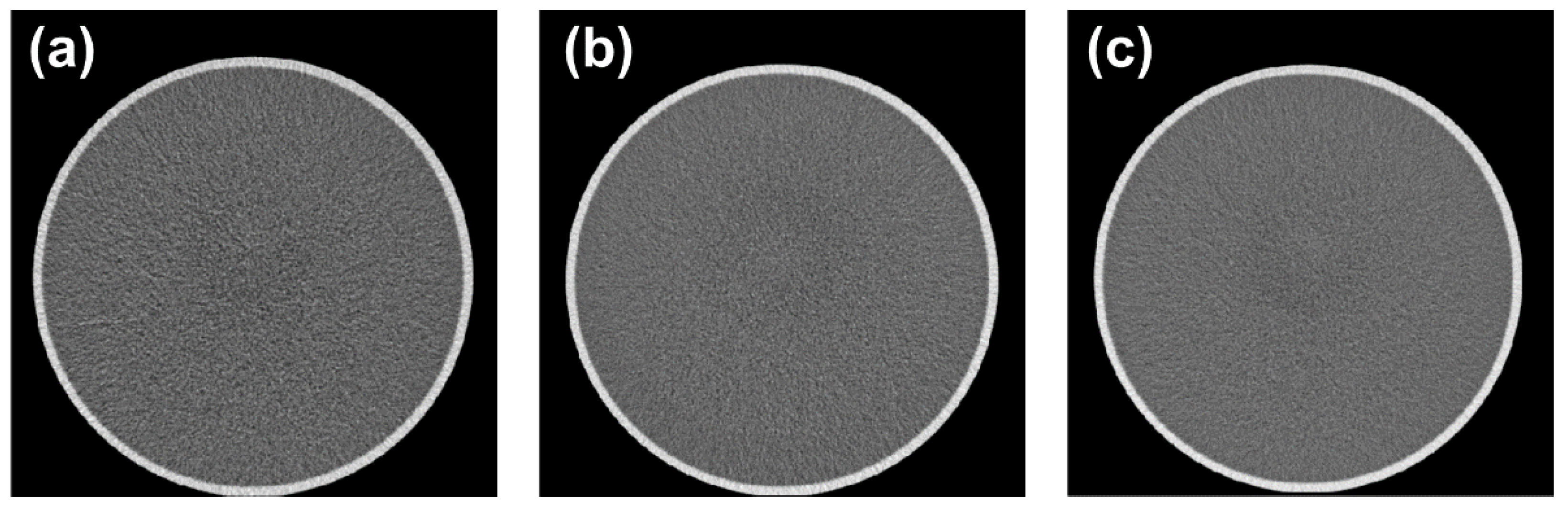
2.1. Phantom Images
2.2. Bilateral Filter
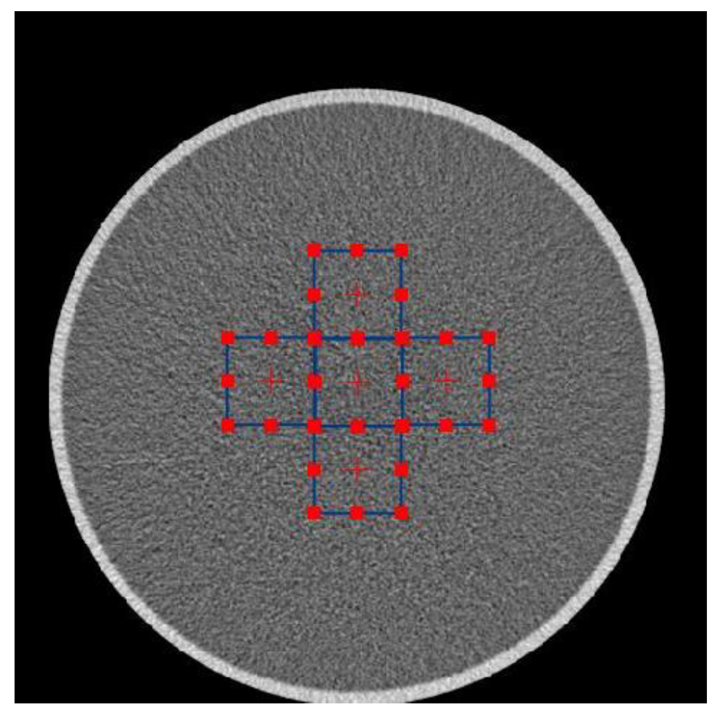
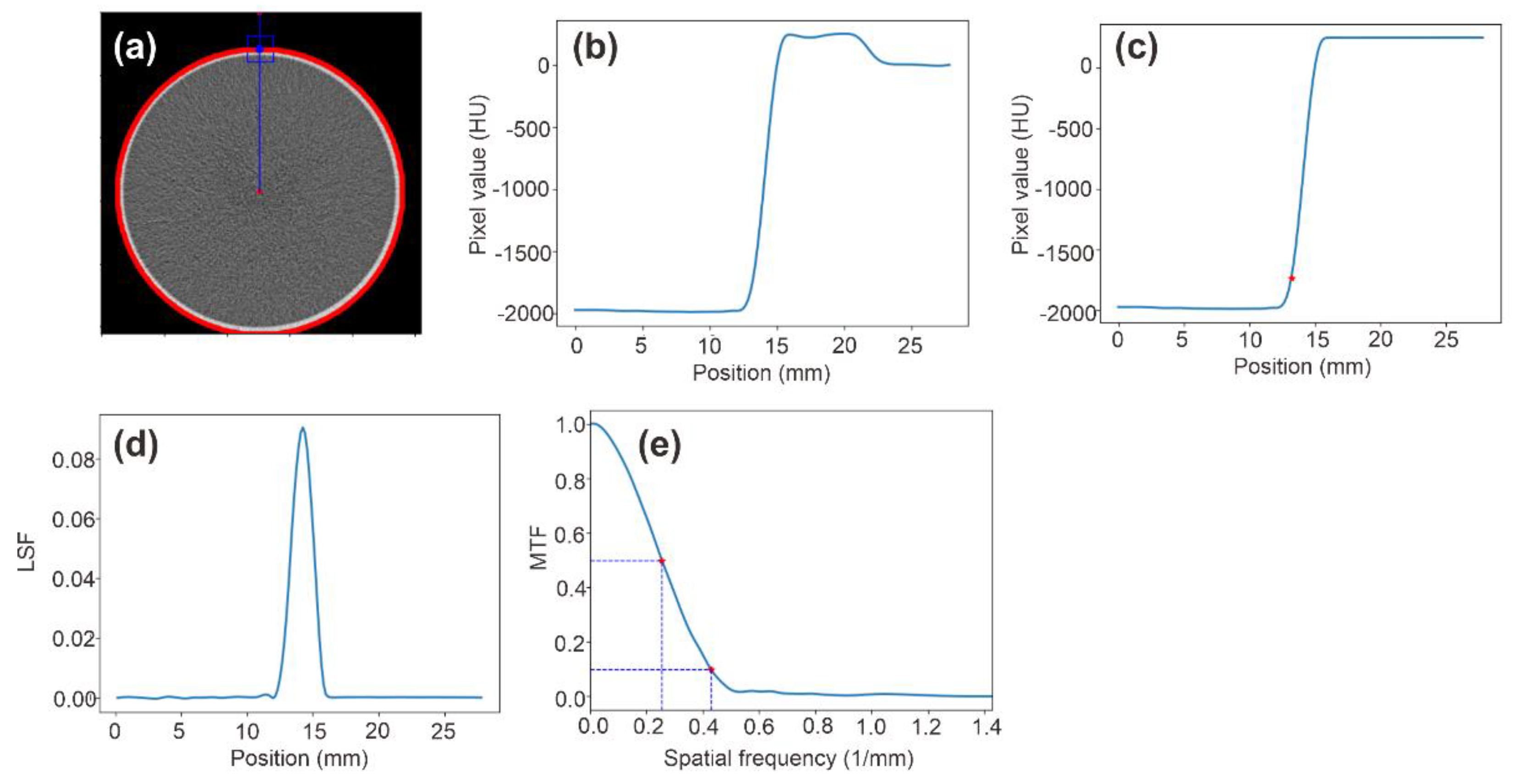
2.3. Implementation of Bilateral Filter, Measurement of Noise Power Spectrum and Spatial Resolution
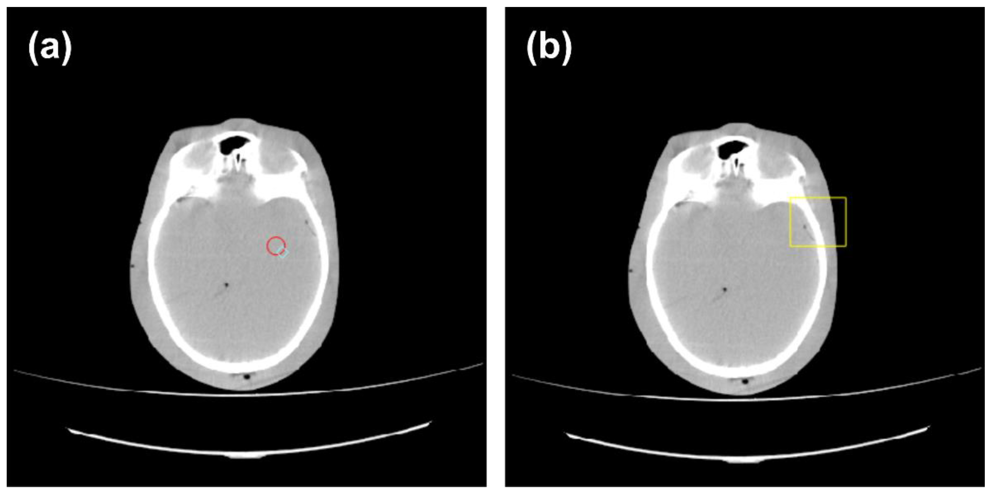
2.4. Implementation of Anthropomorphic Phantom Images
3. Results
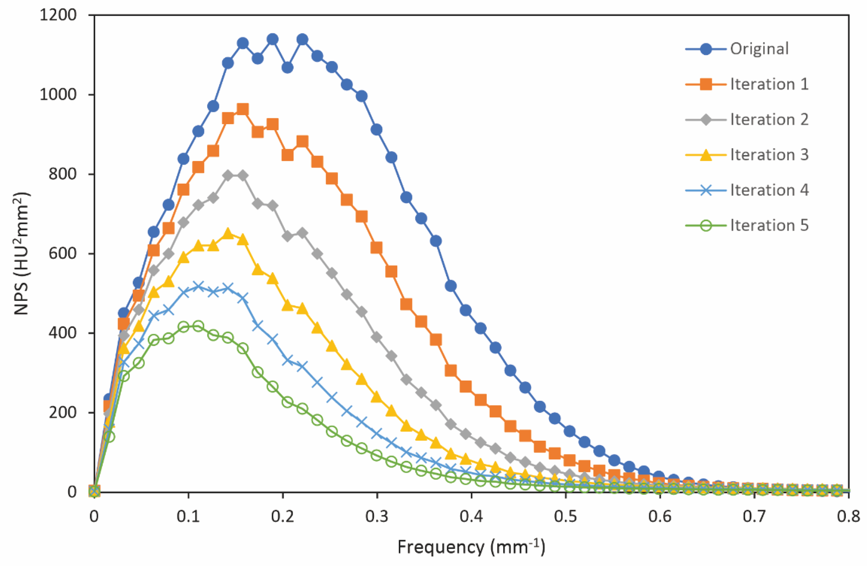
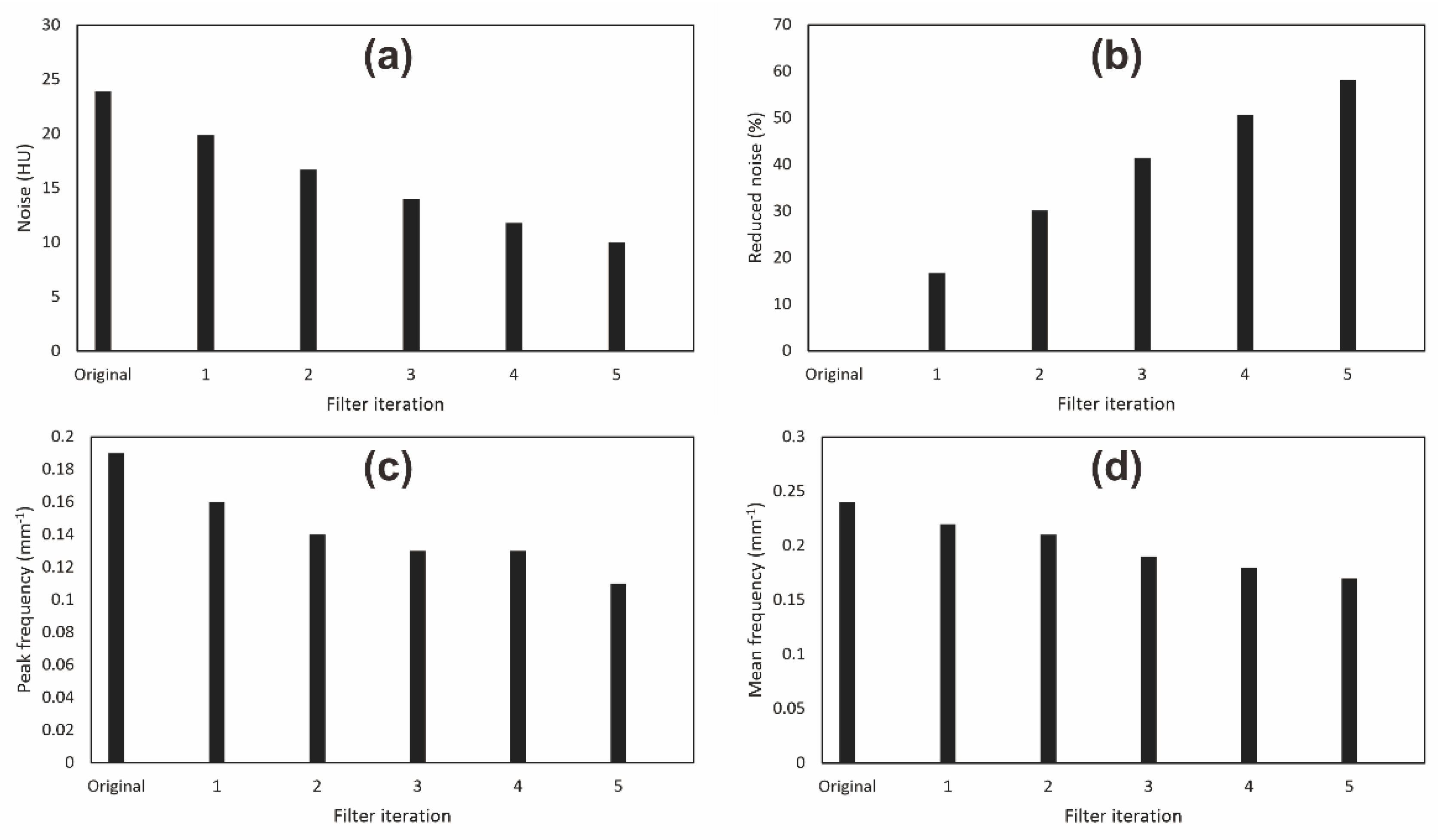
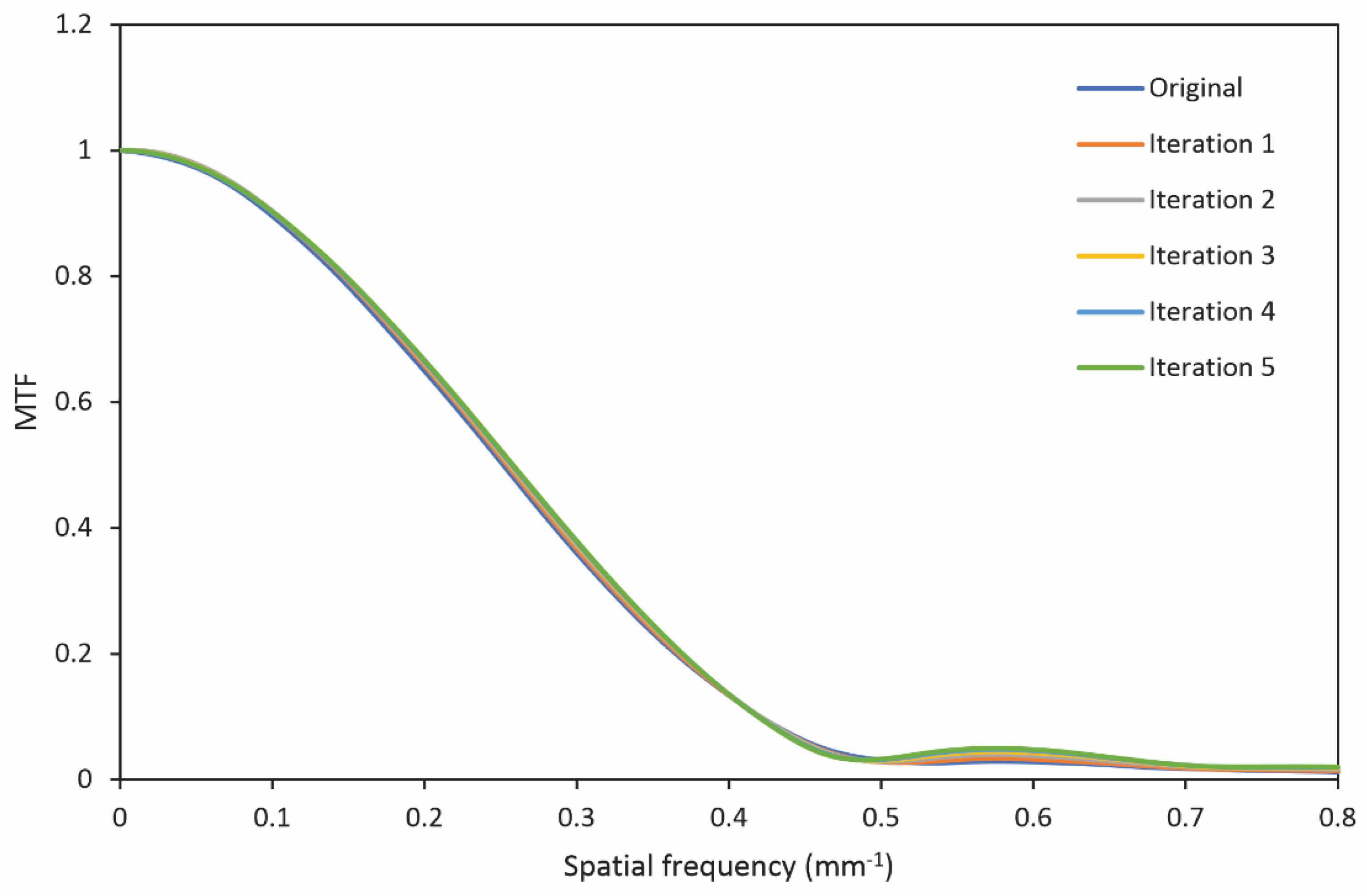
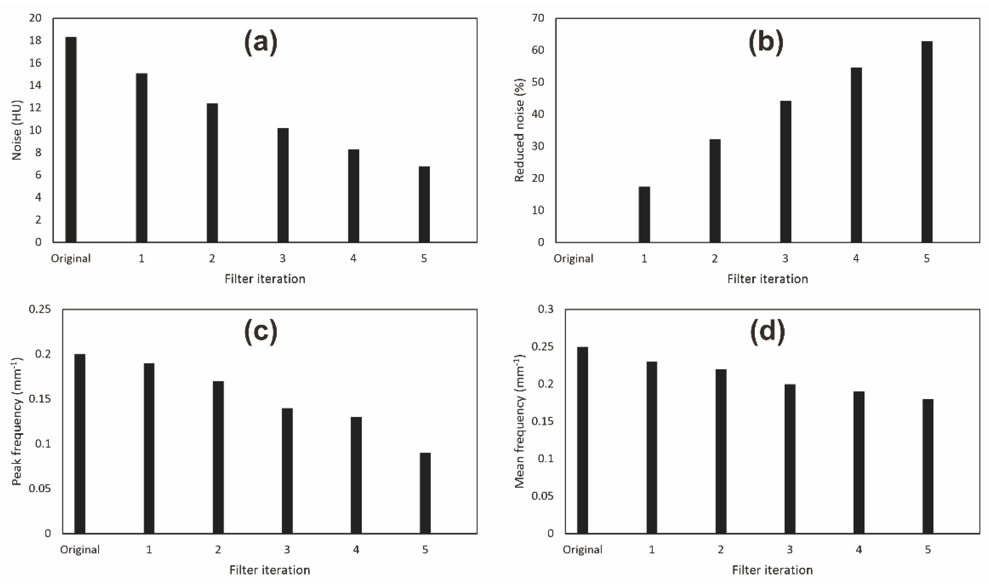
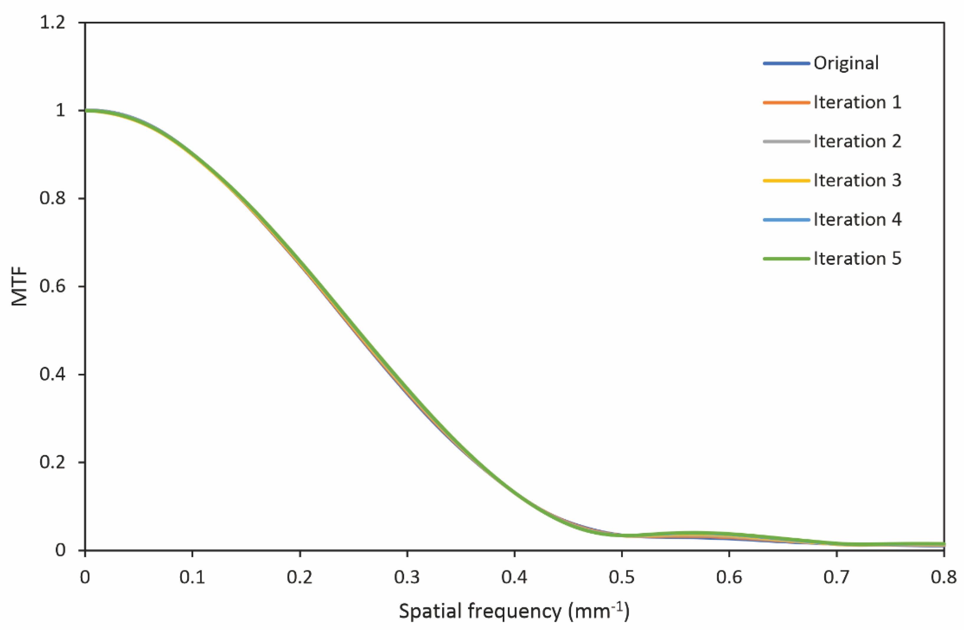
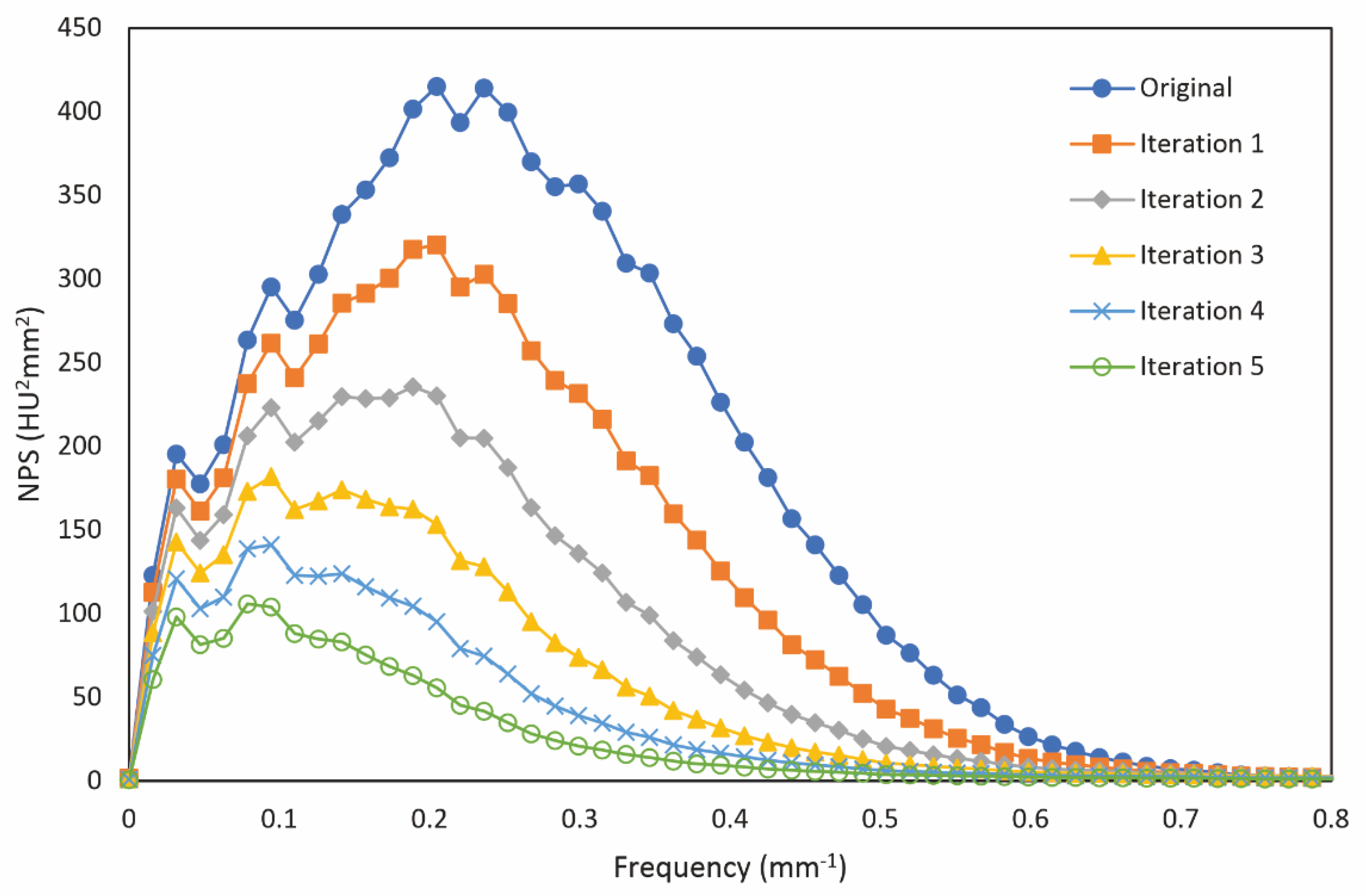
3.1. Tube Current of 77 mAs
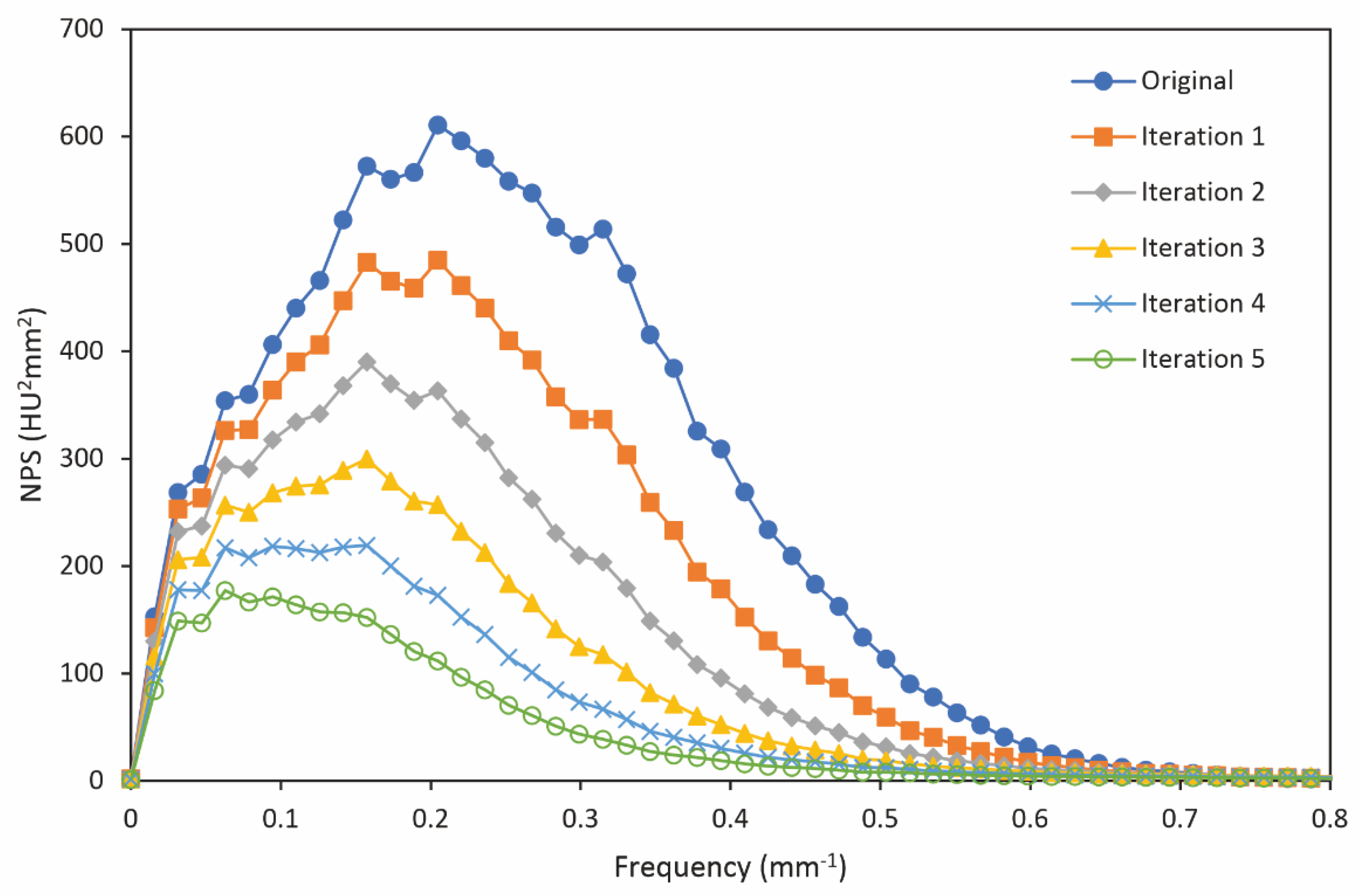
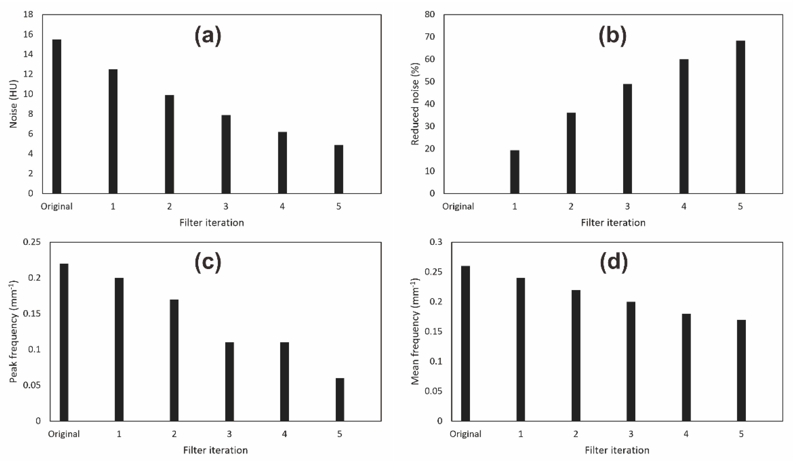
3.2. Tube Current of 154 mAs
3.3. Tube Current of 231 mAs
3.4. Impact of Bilateral Filter on Anthropomorphic Images
4. Discussion
5. Conclusions
Author Contributions
Funding
Data Availability Statement
Conflicts of Interest
References
- Pearce, M.S.; Salotti, J.A.; Little, M.P.; McHugh, K.; Lee, C.; Kim, K.P.; Howe, N.L.; Ronckers, C.M.; Rajaraman, P.; Craft, A.W. Radiation exposure from CT scans in childhood and subsequent risk of leukaemia and brain tumours: A retrospective cohort study. Lancet 2012, 380, 499–505. [Google Scholar] [CrossRef]
- Albert, J.M. Radiation risk from CT: Implications for cancer screening. Am. J. Roentgenol. 2013, 201, W81–W87. [Google Scholar] [CrossRef] [PubMed]
- Chen, J.X.; Kachniarz, B.; Gilani, S.; Shin, J.J. Risk of malignancy associated with head and neck CT in children: A systematic review. Otolaryngol.–Head Neck Surg. 2014, 151, 554–566. [Google Scholar] [CrossRef] [PubMed]
- Yeung, A.W.K. The “As Low As Reasonably Achievable” (ALARA) principle: A brief historical overview and a bibliometric analysis of the most cited publications. Radioprotection 2019, 54, 103–109. [Google Scholar] [CrossRef]
- Ning, P.; Zhu, S.; Shi, D.; Guo, Y.; Sun, M. X-ray dose reduction in abdominal computed tomography using advanced iterative reconstruction algorithms. PLoS ONE 2014, 9, e92568. [Google Scholar] [CrossRef] [PubMed]
- Barreto, I.; Verma, N.; Quails, N.; Olguin, C.; Correa, N.; Mohammed, T.L. Patient size matters: Effect of tube current modulation on size-specific dose estimates (SSDE) and image quality in low-dose lung cancer screening CT. J. Appl. Clin. Med. Phys. 2020, 21, 87–94. [Google Scholar] [CrossRef]
- Whitebird, R.R.; Solberg, L.I.; Bergdall, A.R.; López-Solano, N.; Smith-Bindman, R. Barriers to CT Dose Optimization: The Challenge of Organizational Change. Acad. Radiol. 2021, 28, 387–392. [Google Scholar] [CrossRef]
- Li, Z.; Yu, L.; Trzasko, J.D.; Lake, D.S.; Blezek, D.J.; Fletcher, J.G.; McCollough, C.H.; Manduca, A. Adaptive nonlocal means filtering based on local noise level for CT denoising. Med. Phys. 2014, 41, 011908. [Google Scholar] [CrossRef]
- Anam, C.; Adi, K.; Sutanto, H.; Arifin, Z.; Budi, W.S.; Fujibuchi, T.; Dougherty, G. Noise reduction in CT images using a selective mean filter. J. Biomed. Phys. Eng. 2020, 10, 623–634. [Google Scholar] [CrossRef]
- Cropp, R.J.; Seslija, P.; Tso, D.; Thakur, Y. Scanner and kVp dependence of measured CT numbers in the ACR CT phantom. J. Appl. Clin. Med. Phys. 2013, 14, 338–349. [Google Scholar] [CrossRef]
- Einstein, S.A.; Rong, X.J.; Jensen, C.T.; Liu, X. Quantification and homogenization of image noise between two CT scanner models. J. Appl. Clin. Med. Phys. 2020, 21, 174–178. [Google Scholar] [CrossRef] [PubMed]
- Takenaga, T.; Katsuragawa, S.; Goto, M.; Hatemura, M.; Uchiyama, Y.; Shiraishi, J. Modulation transfer function measurement of CT images by use of a circular edge method with a logistic curve-fitting technique. Radiol. Phys. Technol. 2015, 8, 53–59. [Google Scholar] [CrossRef] [PubMed]
- Wang, J. Construction of local nonlinear filter without staircase effect in image restoration. Appl. Anal. 2011, 90, 1257–1273. [Google Scholar] [CrossRef]
- Masoomi, M.A.; Al-Shammeri, I.; Kalafallah, K.; Elrahman, H.M.; Ragab, O.; Ahmed, E.; Al-Shammeri, J.; Arafat, S. Wiener filter improves diagnostic accuracy of CAD SPECT images-comparison to angiography and CT angiography. Medicine 2019, 98, e14207. [Google Scholar] [CrossRef] [PubMed]
- Vasilache, S.; Ward, K.; Cockrell, C.; Ha, J.; Najarian, K. Unified wavelet and Gaussian filtering for segmentation of CT images; application in segmentation of bone in pelvic CT images. BMC Med. Inform. Decis. Mak. 2009, 9 (Suppl. 1), S8. [Google Scholar] [CrossRef]
- Patil, P.D.; Kumbhar, A.D. Bilateral Filter for Image Denoising. In Proceedings of the 2015 International Conference on Green Computing and Internet of Things (ICGCIoT), Greater Noida, India, 8–10 October 2015; pp. 299–302. [Google Scholar]
- Zhang, M.; Gunturk, B.K. Multiresolution bilateral filtering for image denoising. IEEE Trans. Image Process. 2008, 17, 2324–2333. [Google Scholar] [CrossRef]
- Zhang, B.; Allebach, J.P. Adaptive bilateral filter for sharpness enhancement and noise removal. IEEE Trans. Image Process. 2008, 17, 664–678. [Google Scholar] [CrossRef]
- Joseph, J.; Periyasami, R. An image driven bilateral filter with adaptive range and spatial parameters for denoising Magnetic Resonance Images. Comput. Electr. Eng. 2018, 6, 782–795. [Google Scholar] [CrossRef]
- Zheng, Y.; Fu, H.; Au, O.K.-C.; Tai, C.-L. Bilateral Normal Filtering for Mesh Denoising. IEEE Trans. Vis. Comput. Graph. 2011, 17, 1521–1530. [Google Scholar] [CrossRef]
- Peng, H.; Rao, R. Bilateral kernel parameter optimization by risk minimization. In Proceedings of the IEEE International Conference on Image Processing, Hong Kong, China, 26–29 September 2010; pp. 3293–3296. [Google Scholar]
- Akar, S.A. Determination of optimal parameters for bilateral filter in brain MR image denoising. Appl. Soft Comput. 2016, 43, 87–96. [Google Scholar] [CrossRef]
- Ghosh, S.; Nair, P.; Chaundhury, K.N. Optimized Fourier Bilateral Filtering. IEEE Signal Process. Lett. 2018, 25, 1555–1559. [Google Scholar] [CrossRef]
- Xu, H.; Zhang, Z.; Gao, Y.; Liu, H.; Xie, F.; Li, J. Adaptive Bilateral Texture Filter for Image Smoothing. Front. Neurorobot. 2022, 16, 729924. [Google Scholar] [CrossRef] [PubMed]
- Bronstein, M.M. Lazy Sliding Window Implementation of the Bilateral Filter on Parallel Architectures. IEEE Trans. Image Process. 2011, 20, 1751–1756. [Google Scholar] [CrossRef][Green Version]
- Galiano, G.; Velasco, J. On a Fast Bilateral Filtering Formulation Using Functional Rearrangements. J. Math. Imaging Vis. 2015, 53, 346–363. [Google Scholar] [CrossRef]
- Paris, S.; Kornprobst, P.; Tumblin, J.; Durand, F. Bilateral Filtering: Theory and Applications. Found. Trends Comput. Graph. Vis. 2009, 4, 1–73. [Google Scholar] [CrossRef]
- Anh, D.N. Iterative Bilateral Filter and Non-Local Mean. Int. J. Comput. Appl. 2014, 106, 33–38. [Google Scholar]
- Zeng, R.; Gavrielides, M.A.; Petrick, N.; Sahiner, B.; Li, Q.; Myers, K.J. Estimating local noise power spectrum from a few FBP-reconstructed CT scans. Med. Phys. 2016, 43, 568–582. [Google Scholar] [CrossRef]
- Li, G.; Liu, X.; Dodge, C.T.; Jensen, C.T.; Rong, X.J. A noise power spectrum study of a new model-based iterative reconstruction system: Veo 3.0. J. Appl. Clin. Med. Phys. 2016, 17, 428–439. [Google Scholar] [CrossRef]
- Dolly, S.; Chen, H.C.; Anastasio, M.; Mutic, S.; Li, H. Practical considerations for noise power spectra estimation for clinical CT scanners. J. Appl. Clin. Med. Phys. 2016, 17, 392–407. [Google Scholar] [CrossRef]
- Park, J.; Han, J.; Lee, B. Performance of bilateral filtering on Gaussian noise. J. Electron. Imag. 2014, 23, 043024. [Google Scholar] [CrossRef]
- Solomon, J.B.; Christianson, O.; Samei, E. Quantitative comparison of noise texture across CT scanners from different manufacturers. Med. Phys. 2012, 39, 6048–6055. [Google Scholar] [CrossRef] [PubMed]
- Samei, E.; Bakalyar, D.; Boedeker, K.L.; Brady, S.; Fan, J.; Leng, S.; Myers, K.J.; Popescu, L.M.; Ramirez Giraldo, J.C.; Ranallo, F.; et al. Performance evaluation of computed tomography systems: Summary of AAPM Task Group 233. Med. Phys. 2019, 46, e735–e756. [Google Scholar] [CrossRef]
- ImQuest. Available online: https://deckard.duhs.duke.edu/~samei/tg233.html (accessed on 10 July 2022).
- Anam, C.; Budi, W.S.; Fujibuchi, T.; Haryanto, F.; Dougherty, G. Validation of the tail replacement method in MTF calculations using the homogeneous and non-homogeneous edges of a phantom. J. Phys. Conf. Ser. 2019, 1248, 012001. [Google Scholar] [CrossRef]
- Anam, C.; Naufal, A.; Fujibuchi, T.; Matsubara, K.; Dougherty, G. Automated development of the contrast-detail curve based on statistical low-contrast detectability in CT images. J. Appl. Clin. Med. Phys. 2022, 9, e13719. [Google Scholar] [CrossRef]
- Anam, C.; Arif, I.; Haryanto, F.; Lestari, F.P.; Widita, R.; Budi, W.S.; Sutanto, H.; Adi, K.; Fujibuchi, T.; Dougherty, G. An improved method of automated noise measurement system in CT images. J. Biomed. Phys. Eng. 2021, 11, 163–174. [Google Scholar] [PubMed]
- Mendrik, A.M.; Vonken, E.J.; van Ginneken, B.; de Jong, H.W.; Riordan, A.; van Seeters, T.; Smit, E.J.; Viergever, M.A.; Prokop, M. TIPS bilateral noise reduction in 4D CT perfusion scans produces high-quality cerebral blood flow maps. Phys. Med. Biol. 2011, 56, 3857–3872. [Google Scholar] [CrossRef] [PubMed]
- Buades, A.; Coll, B.; Morel, J.M. The staircasing effect in neighborhood filters and its solution. IEEE Trans. Image Process. 2006, 15, 1499–1505. [Google Scholar] [CrossRef] [PubMed]
- Al-Hinnawi, A.R.; Daear, M.; Huwaijah, S. Assessment of bilateral filter on 1/2-dose chest-pelvis CT views. Radiol. Phys. Technol. 2013, 6, 385–398. [Google Scholar] [CrossRef] [PubMed]
- Buades, A.; Coll, B.; Morel, J.M. A non-local algorithm for image denoising. In Proceedings of the IEEE Computer Society Conference on Computer Vision and Pattern Recognition (CVPR’05), San Diego, CA, USA, 20–25 June 2005; Volume 2, pp. 60–65. [Google Scholar]
- Stiller, W. Basics of iterative reconstruction methods in computed tomography: A vendor-independent overview. Eur. J. Radiol. 2018, 109, 147–154. [Google Scholar] [CrossRef]
- McLeavy, C.M.; Chunara, M.H.; Gravell, R.J.; Rauf, A.; Cushnie, A.; Talbot, C.S.; Hawkins, R.M. The future of CT: Deep learning reconstruction. Clin. Radiol. 2021, 76, 407–415. [Google Scholar] [CrossRef]


| Parameter | Value |
|---|---|
| Scanner | Neusoft NeuViz 16 Classic |
| Tube current (mAs) | 77, 154, 231 |
| Tube voltage (kVp) | 120 |
| Slice thickness (mm) | 5 |
| Scan option | Helical |
| Pitch | 1.2 |
| Convolution kernel | F20 |
| Image reconstruction | Filtered-back projection |
| Parameter | Value |
|---|---|
| Scanner | Toshiba Alexion |
| Tube current (mAs) | 100 |
| Tube voltage (kVp) | 120 |
| Slice thickness (mm) | 7 |
| Scan option | Helical |
| Pitch | 1.5 |
| Convolution kernel | FC13 |
| Image reconstruction | Filtered-back projection |
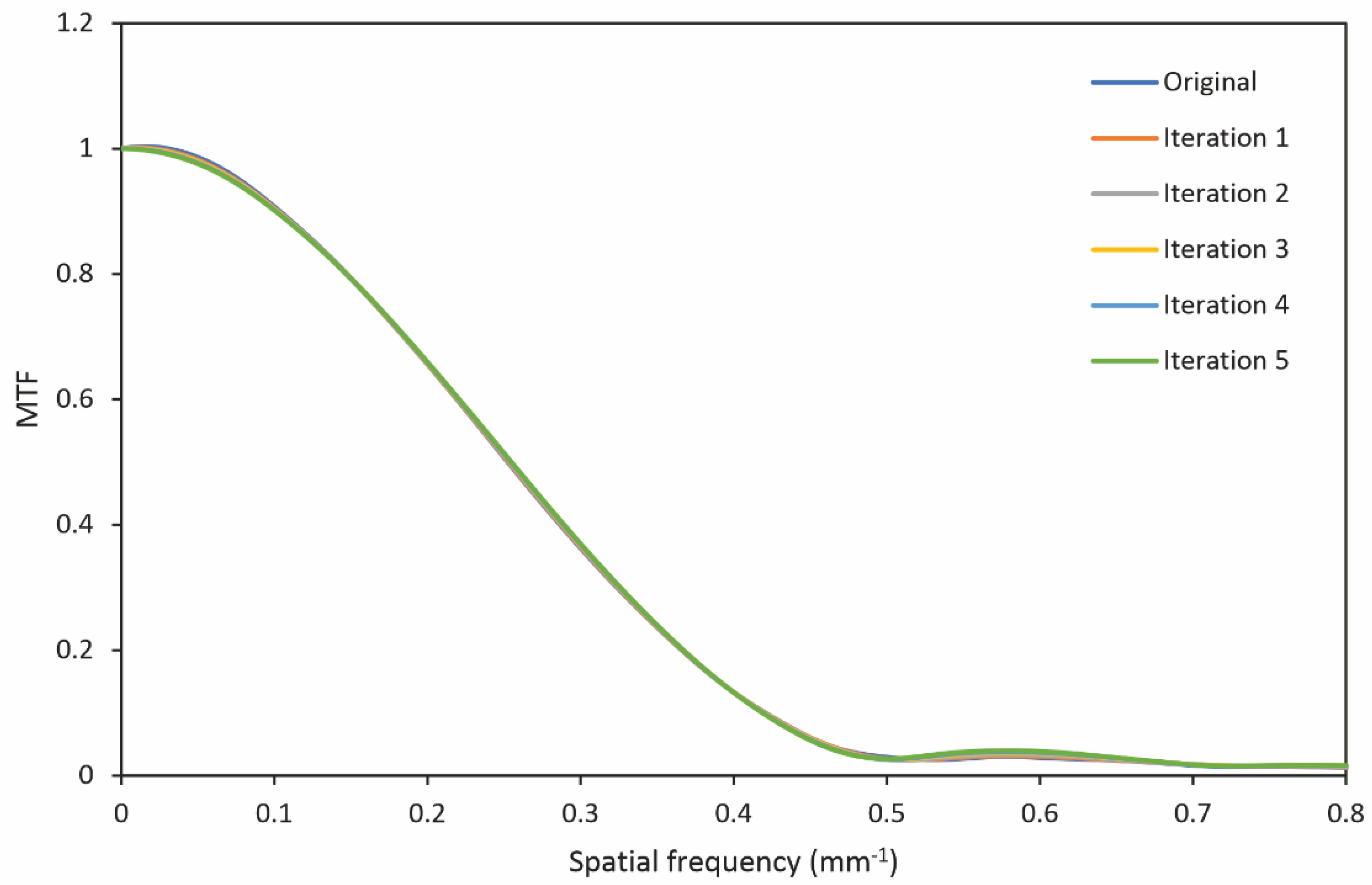
| Filter Iteration | MTF50 (mm−1) | MTF10 (mm−1) |
|---|---|---|
| Original | 0.25 | 0.42 |
| 1 | 0.25 | 0.42 |
| 2 | 0.26 | 0.42 |
| 3 | 0.26 | 0.42 |
| 4 | 0.26 | 0.42 |
| 5 | 0.26 | 0.42 |
| Filter Iteration | MTF50 (mm−1) | MTF10 (mm−1) |
|---|---|---|
| Original | 0.25 | 0.42 |
| 1 | 0.25 | 0.42 |
| 2 | 0.25 | 0.42 |
| 3 | 0.25 | 0.42 |
| 4 | 0.25 | 0.42 |
| 5 | 0.25 | 0.42 |
| Filter Iteration | MTF50 (mm−1) | MTF10 (mm−1) |
|---|---|---|
| Original | 0.25 | 0.42 |
| 1 | 0.25 | 0.42 |
| 2 | 0.25 | 0.42 |
| 3 | 0.25 | 0.42 |
| 4 | 0.25 | 0.42 |
| 5 | 0.25 | 0.42 |
| Filter Iteration | SSIM |
|---|---|
| 1 | 0.85 |
| 2 | 0.69 |
| 3 | 0.60 |
| 4 | 0.54 |
| 5 | 0.50 |
Publisher’s Note: MDPI stays neutral with regard to jurisdictional claims in published maps and institutional affiliations. |
© 2022 by the authors. Licensee MDPI, Basel, Switzerland. This article is an open access article distributed under the terms and conditions of the Creative Commons Attribution (CC BY) license (https://creativecommons.org/licenses/by/4.0/).
Share and Cite
Anam, C.; Naufal, A.; Sutanto, H.; Adi, K.; Dougherty, G. Impact of Iterative Bilateral Filtering on the Noise Power Spectrum of Computed Tomography Images. Algorithms 2022, 15, 374. https://doi.org/10.3390/a15100374
Anam C, Naufal A, Sutanto H, Adi K, Dougherty G. Impact of Iterative Bilateral Filtering on the Noise Power Spectrum of Computed Tomography Images. Algorithms. 2022; 15(10):374. https://doi.org/10.3390/a15100374
Chicago/Turabian StyleAnam, Choirul, Ariij Naufal, Heri Sutanto, Kusworo Adi, and Geoff Dougherty. 2022. "Impact of Iterative Bilateral Filtering on the Noise Power Spectrum of Computed Tomography Images" Algorithms 15, no. 10: 374. https://doi.org/10.3390/a15100374
APA StyleAnam, C., Naufal, A., Sutanto, H., Adi, K., & Dougherty, G. (2022). Impact of Iterative Bilateral Filtering on the Noise Power Spectrum of Computed Tomography Images. Algorithms, 15(10), 374. https://doi.org/10.3390/a15100374