Abstract
In this work, we consider the problem of calculating the generalized Moore–Penrose inverse, which is essential in many applications of graph theory. We propose an algorithm for the massively parallel systems based on the recursive algorithm for the generalized Moore–Penrose inverse, the generalized Cholesky factorization, and Strassen’s matrix inversion algorithm. Computational experiments with our new algorithm based on a parallel computing architecture known as the Compute Unified Device Architecture (CUDA) on a graphic processing unit (GPU) show the significant advantages of using GPU for large matrices (with millions of elements) in comparison with the CPU implementation from the OpenCV library (Intel, Santa Clara, CA, USA).
1. Introduction
The generalized inverses of a matrix are defined as generalizations to the matrix inverse, so a matrix can have a generalized inverse even if the matrix is not regular or square. For nonsingular matrices, the generalized inverse coincides with its ordinary inverse. In this paper, we consider the Moore–Penrose generalized matrix inverse (or the pseudoinverse), which is the oldest type of generalized matrix inverses [1]. Pseudoinverse exists for arbitrary matrices, and one of its most important applications is finding the least square solution to the overdetermined systems of linear equations [2,3,4,5].
The generalized Moore–Penrose inverse finds multiple applications in graph theory. In [6], the authors proved an equation that relates the Moore–Penrose pseudoinverses of two matrices A, B such that A = N−1BM−1 and applied it to the Moore–Penrose inverse representation of the normalized Laplacian of a graph. In [7], the authors considered the Moore–Penrose inverse of an oriented graph incidence matrix. In [8], the same authors presented a combinatorial interpretation of the Moore–Penrose inverse problem for complete multipartite and bi-block graphs. In [9], the authors provided a combinatorial interpretation of the Moore–Penrose inverse of the graph incidence matrix, where blocks are either cliques or cycles, and they described the minors of the Moore–Penrose inverse of the incidence matrix, with the rows indexed by cut edges. In [10], the authors considered the Moore–Penrose inverses of the signless Laplacian and signless edge-Laplacian of a graph and proposed combinatorial formulas of the Moore–Penrose inverses for trees and odd unicyclic graphs.
In addition to the above, the pseudoinverse matrix finds application in many other areas. In [11], the authors considered two security issues for smart devices such as smartphones, tablets, etc., namely changing a shared key between two users and privacy-preserving auditing in cloud storage. Their solution is a one-way method of linear complexity based on the matrix pseudoinverse. Fast computation enables us to apply this method to devices with limited computational capacity. An interesting approach is the application of pseudoinverse and projective matrices in the areas of studying control, observation, and identification problems [12]. The method of the pseudoinverse perturbation, based on matrix splitting, is extended to projective matrices for application in identification, nonlinear regressive analysis, function approximation, and prediction problems.
Many authors [13,14] proposed various methods for applying the Moore–Penrose inversion to restore digital images. In [14], the authors introduced a method for the restoration of images that have been blurred by uniform and nonuniform linear motion. This method is based on the pseudoinverse solution of the matrix equation modeling the motion blur. The method directly generates blurring matrices based on their special structure, without iterative computations, which leads to a decrease in the CPU time, compared with other methods for the pseudoinverse computation. In [13], the authors presented a new approach to the problem of image reconstruction with the use of the Moore–Penrose generalized inverse, which provides a very high-resolution level of the reconstructed image as well as a considerable decrease in the computational load compared with the classic techniques.
The calculation of the pseudoinverse matrix is often necessary when solving forecasting problems. In [15], a flat neural network was considered for the online prediction of engine states using a recursive algorithm based on a pseudoinverse partition matrix. Experimentally, the high accuracy of the developed neural network and its sufficient reliability in real-time forecasting are established, which enables us to use this network for nonlinear systems with multiple inputs and multiple outputs, such as vehicle engines. The problem of prediction was also considered in [16]. The authors proposed a fault diagnosis strategy for a ventilation unit that uses a neural network with a radial basis function to model the causes of faults. As the main ones, the authors chose the Gaussian functions. The parameters of these functions and the network weights were calculated using a new network training method that combines a genetic algorithm and a pseudoinverse matrix algorithm. Algorithm testing showed the successful identification of each artificial fault.
The methods based on pseudoinversion can be used to model the phenomena of various physical natures. The authors of [17] considered the determination of temperature and strain in a single-fiber Brillian Optical Pulse Analyzer (BOTDA) system based on the Moore–Penrose inversion of nonsquare matrices. By comparing the developed method for one optical band with another reference method for two optical bands, the authors experimentally proved that the method under study is suitable for recovering the temperature and strain data with sufficient accuracy. In [18], the methods for obtaining brightness and temperature for synthetic aperture radiometers were considered. The authors proposed one of the inversion methods for the general equation to use the pseudoinverse matrix method. The authors of [19] presented an incremental pseudoinverse matrix calculation method applicable to machine learning and computational neuroscience, which, according to the authors, is a biologically plausible learning method and can be adapted for nonstationary data flows. The authors claimed that the presented method is significantly more memory-efficient than the usual calculation of pseudoinverses through singular value decomposition. In [20], the algorithms for the formation of control actions in control systems of dynamic objects were studied. To find a solution, the authors used stable algorithms based on orthogonal expansions and the pseudoinversion of square matrices, which contribute to an increase in the accuracy of the formation of control actions. In [21], two models of discrete-time Taylor-type neural networks for the pseudoinversion of a time-varying matrix were proposed. Additionally, examples of these models were given and analyzed to generate the manipulator’s movement. The study was continued in [22], where the authors used two simplified nonlinear activation functions. Compared with the models from [21], these two simplified models achieved faster finite-time convergence and possess better robustness. Comparative simulations and examples in engineering applications show the advantage of these two new models for solving the time-varying matrix pseudoinverse problems.
Numerous computational methods have been developed for the generalized inverse of a matrix, from Newton-type iterative methods [23,24,25,26,27] to finite algorithms [28,29,30]. The finite algorithms are based on the generalized inverse computation of the rank-one modified matrix. For example, in [29], the authors presented a recursive procedure to compute the Moore–Penrose inverse of a matrix A based on the symmetric rank-one updates. The singular value decomposition and full-rank decomposition enable us to calculate the pseudoinverse [31,32]. In addition, the QR decomposition is a useful tool for calculating generalized inverses [33].
One of the methods of computing the inverse of a nonsingular matrix A is the Gauss–Jordan elimination procedure [28]. In [34,35,36], the authors presented an alternative expression for the matrix pseudoinverse. Based on this expression, the authors proposed a Gauss–Jordan elimination method for the computation of A†.
In our work, based on the recursive algorithm given in [28], we propose a recursive algorithm for the parallel computing architecture CUDA (Compute Unified Device Architecture, Nvidia, Santa Clara, CA, USA), where a massively parallel system performs the most computationally expensive operations of matrix multiplication. The computations were performed with a graphic processing unit (GPU). Even though GPU cores are simpler and have fewer functionalities and show far worse performance than CPU cores, GPUs can have thousands of cores, which makes them suitable for computations applicable to parallelizable calculations.
The structure of this paper is as follows: In Section 2, we give a formal definition and some of the properties of the Moore–Penrose generalized inverse; Section 3 represents the specific features of GPU programming and CUDA. In Section 4, we state the algorithm from [28], while in Section 5, we introduce the algorithm for massively parallel systems in CUDA. In Section 6, we compare the execution time of the implemented algorithm and that of an algorithm from the OpenCV library, which runs on the CPU. Section 7 represents the conclusion.
2. Moore–Penrose Generalized Inverse
In this section, we give a brief introduction to the Moore–Penrose pseudoinverse, a generalization of the matrix inverse.
Definition 1
([37]). The inverse of a given regular square matrix A ∈ Cn×n is a square matrix A−1 such that
where In is the n × n identity matrix.
AA−1 = In, A−1A = In,
A square matrix A ∈ Cn×n has a unique inverse if det(A) ≠ 0. If A has an inverse, we say that A is a nonsingular (regular) matrix. Otherwise, we say that A is a singular matrix.
One of the basic and the most important applications of a matrix inverse is in solving a system of linear equations
where A ∈ Rm×n and b ∈ Rm. If A is regular, the solution to the system (1) is given by
Ax = b,
x = A−1b.
However, by Definition 1, the inverse can exist only for regular square matrices (satisfying m = n). Generalized inverses are introduced to overcome these restrictions of the ordinary inverse [1]. System (1) has at least one solution if b ∈ R(A), where R(A) = {y| ∃ x ∈ Rm, Ax = y}. In other words, b ∈ R(A) if there exists a matrix X ∈ Rn×m such that x = Xb is a solution to the linear equations system. The matrix X can be described using the following Penrose equations [38]:
AXA = A, (a)
XAX = X, (b)
(AX) * = AX, (c)
(XA)*= XA. (d)
XAX = X, (b)
(AX) * = AX, (c)
(XA)*= XA. (d)
A matrix X, X ∈ Rn×m that satisfies (c) is called the Moore–Penrose generalized inverse of matrix A or the pseudoinverse of matrix A and is denoted by A†. The authors of [38] proved that the linear equation system (3) has a unique solution for the arbitrary matrix A.
If A is a regular square matrix, its inverse, A−1, satisfies the equations in (3), and it is equal to pseudoinverse A†. Sometimes, we may need to find a matrix X that satisfies only some equation from 3. For an array S of elements from {1, 2, 3, 4}, the set of matrices that satisfies the equations from 3 indexed by elements from S is denoted by A{S} (if S = {1, 2, 3, 4}; the set A{S} has exactly one element, A{S} = {A†}).
3. Massively Parallel Computing and CUDA
GPUs are traditionally used for the fast generation and manipulation of images by splitting the massive computation task into tiny operations on a small volume of data performed in parallel threads. Usually, each thread is related to a single pixel. This technology was adjusted for parallel computing on many cores. Using GPUs for general-purpose computing was made accessible in 2006 when NVidia released the first version of the CUDA platform [39] with indirect access to the instructions and memory for parallel computation on GPUs.
The code of a CUDA program contains the host code that is executed on a CPU and the device code that is executed on a GPU. The host and the device have distinct memories and address spaces, and the device memory is managed by built-in functions. In most cases, we can identify three main steps in the execution flow of a CUDA program: copying the memory from the CPU to GPU, the function calls and the execution of functions that are executed on the GPU, and copying the results from the GPU to CPU [39].
The procedures and functions that are executed on the GPU in parallel are called kernels (keyword _global_ in their declaration). The most important factor in a parallel version of the algorithm is the execution of the most expensive calculations using the kernel functions and avoiding heavy information traffic between the GPU and the host device.
The kernel body, using the CUDA programming model, is executed in parallel with many threads grouped in blocks, which are further grouped in a grid. The maximum number of threads one block can contain is 1024. The CUDA allows blocks and grids to be organized in one, two, or three dimensions. Every thread has a unique identifier within the block, which can be accessed through the built-in threadIdx, which contains x, y, and z attributes. Similarly, each thread can access the blockIdx variable. The dimensions of the block and grid can be accessed through the built-in variables blockDim and gridDim. We use the following formulas to identify a thread within a block and a block within a grid:
where (Bx, By, Bz) and (Gx, Gy, Gz) are the dimensions of the block and grid, respectively, and xt, yt, and zt and xb, yb, and zb represent the threadIdx.x, threadIdx.y, threadIdx.z, blockIdx.x, blockIdx.y, and blockIdx.z, respectively. We can easily calculate the unique global thread ID as:
where bid and tid represent the unique thread ID within the block and block ID, respectively.
uniqueThreadIdWithinBlock = xt + ytBx + ztBxBy,
uniqueBlockId = xb + ybGx + zbGxGy,
uniqueGlobalThreadId = Nbbid + tid,
The GPU contains various types of programmable and nonprogrammable memories. L1 cache, constant cache, L2 cache, and read-only cache are types of nonprogrammable GPU memory. The programmable types of GPU memory are global memory, shared memory, and registers [39]. Global memory is the largest and slowest. Optimizing access to global memory is crucial to improving the program’s performance.
Shared memory (programmable cache) is a fast memory shared by all the threads within the same block and is visible to all these threads within the same block. It is divided into 32 equally sized banks. Different memory banks can be accessed simultaneously, so it is important to organize the data so that different threads access different shared memory banks. Its address space is one-dimensional, and assuming that we store 4-byte values, the kth bank contains elements such that i mod 32 = k, where i is the index of the data in shared memory. The optimal use of shared memory is crucial for overall performance. In general, the bank index is calculated as
bankIndex = (byteAddress/4) mod 32.
The CUDA offers a few types and levels of synchronization. The most important is the synchronization between the threads of the same block and between different kernels. The execution of each thread that invokes the _syncthreads() function is blocked until all the threads of the same block execute the same function. The concurrency and synchronization between the different kernels, the host, and the device or the memory transfer between the host and the device and the execution of the device code can be achieved using the CUDA Streams and Events. The operations in different streams are executed in parallel, while the operations from the same stream are executed sequentially.
4. Recursive Algorithm for Calculating the Pseudoinverse
This section describes a recursive algorithm for calculating the Moore–Penrose generalized inverse [28]. A few algorithms and results from other papers [40,41,42] are combined to produce this algorithm. In the following subsections (similarly to the structure of [28]), we list the auxiliary algorithms used to calculate the pseudoinverse.
4.1. Generalized Cholesky Factorisation
This subsection presents the algorithm for the recursive calculation of the generalized Cholesky factorization [43] of an arbitrary positive semidefinite matrix. If a given matrix A is positive definite, there exists an upper triangular matrix U such that A = UTU. By generalizing the Cholesky factorization, it is possible to calculate the unique matrix U even if A is positive semidefinite. The existence and uniqueness of such a matrix are verified in [41].
The recursive generalized Cholesky factorization is taken from [28], and it calculates the matrix U and its inverse matrix Y = U−1 (Figure 1). The symmetric positive semidefinite n × n matrix A is the input. Matrices U and Y defined by A = UTU and Y = U−1 are the output.
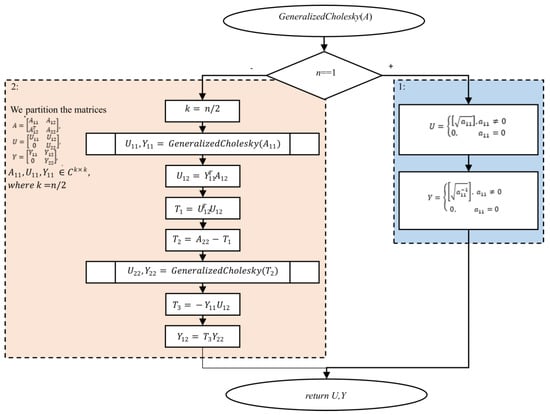
Figure 1.
Algorithm 4.1 (Figure A1) Recursive generalized Cholesky factorization.
If we implement matrix multiplications in Algorithm 4.1 (Figure 1) in the time complexity of O(n2+∈), 0 < ∈ < 1, the complexity of this algorithm is also O(n2+∈). The memory complexity of the algorithm is Θ(n2) [28].
4.2. Strassen’s Matrix Inverse Algorithm
The block diagram of Strassen’s matrix inverse algorithm (Figure 2) is based on the pseudocode taken from [28] and is originally stated in [40]. The input is a regular n × n matrix A, in which all the main diagonal minors are regular. The algorithm returns the inverse matrix X = A−1.
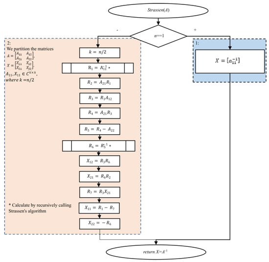
Figure 2.
Algorithm 4.2 (Figure A2): Strassen’s matrix inverse algorithm. Recursion calls are marked with “*”.
As in Algorithm 4.1, we assume that the matrix product complexity is O(n2+∈), 0 < ∈ < 1; the complexity of Algorithm 4.2 is O(n2+∈), while the memory complexity is Θ(n2). The proof is presented in [28]. The original Strassen’s matrix inverse algorithm uses Stassen’s matrix multiplication algorithm to multiply the matrices, which has a time complexity of O(nlog7) ≈ O(n2.8074).
4.3. Calculating the Pseudoinverse
The following lemma [42] provides the basis for the algorithm used in this work.
Lemma 1.
Let A be real m × n matrix and STS generalized Cholesky factorization of matrix ATA. If matrix LT is obtained by dropping the zero rows of matrix S, the Moore–Penrose generalized inverse of matrix A satisfies the following equation:
A† = L(LTL)−1(LTL)−1LTAT.
To calculate the pseudoinverse in the same time complexity as matrix multiplication, in [28], the inverse of (LTL)−1 is calculated by using Algorithm 4.2, and matrix S is computed using Algorithm 4.1. That way, we come to Algorithm 4.3 (Figure 3) for calculating the pseudoinverse [28].
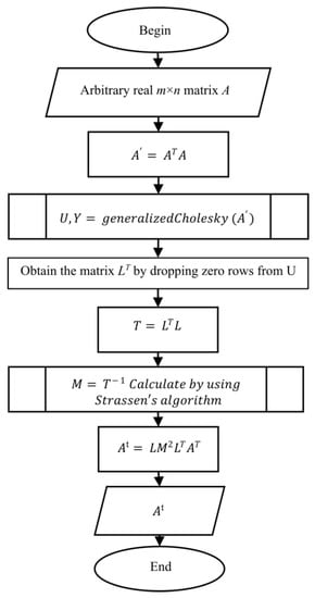
Figure 3.
Algorithm 4.3 (Figure A3): Computing the pseudoinverse in matrix multiplication time complexity.
5. Algorithm for Massively Parallel Systems
This section presents the massively parallel (CUDA) version of the algorithm described in Section 4. The important parts of the code or functions are given in the listings available in Appendix A, as indicated in [44].
5.1. Representing a Matrix in GPU Memory
A way to store a matrix in the GPU memory is by using a 1D array and arranging the elements in a row-major or column-major order. We implement the matrices in the row-major order, so the matrix is accessed using the index calculated from the row and column index as index = i × m + j, where i, j, and m represent the row index, the column index, and the number of columns in a given matrix, respectively. Since we cannot access the array values (stored in the GPU memory) from the host (CPU), we need to copy the array from the device to the host first. To hide index mapping and memory management, the matrix is accessed through the Matrix class (a class template Matrix<T>, where T is the type of values stored in the matrix). Parts of the Matrix class template is listed in [44].
To enable the fast partitioning of a matrix, we implemented a get_submatrix() method, which does not copy the memory but only assigns the pointer, offset, and row stride attributes. The attributes row stride is used to specify how many elements we must ”skip” when moving from one row to another. Note that the row stride does not have to be equal to the number of columns (attribute m) because a matrix can be created as a submatrix of a larger matrix. However, both matrices will share the same pointer to a 1D array. Implemented this way, a matrix can be partitioned in O(1) time complexity. The rest of the class functionalities can be deduced from the names of the methods or static functions and the names and argument types.
The functions or methods that take the CUDA stream as an argument can be executed in a separate stream synchronically or asynchronically, depending on the sync argument. This holds for all methods or functions.
5.2. Matrix Multiplication
The matrix multiplication implementation is based on the implementation from the CUDA Programming Guide [45]. In Figure 4, the organization of the calculations is presented when executing a parallel algorithm for matrix multiplication based on the division of matrices by rows.
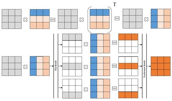
Figure 4.
Matrix multiplication: CUDA implementation. Parts of the input and output matrices processed by CUDA threads are given in different colors.
All the index calculations are hidden by using the get_element() and set_element() methods, and each matrix can be transposed. The implementation of the matrix multiplication kernel matmul_kernel() [44] and the wrapping matmul() function are provided in [44]. When accessing global memory, all the reads and writes are coalesced and aligned, and there are no bank conflicts when accessing shared memory. This rule holds regardless of whether some matrix is transposed.
We also tested our pseudoinverse calculation algorithm with a matrix multiplication algorithm from the cuBLAS library.
In Figure 4, the organization of calculations is presented when executing a parallel algorithm for matrix multiplication based on the division of matrices by rows.
5.3. Implementation of Cholesky Factorization
The pseudocode shows the implementation of the generalized Cholesky factorization based on Algorithm 4.1 (Appendix A, Figure A1). The matrices A, U, and Y need to be square matrices. If a 1 × 1 matrix is passed as an argument, we need to call a specialized kernel function that sets the value of U and Y according to Step 1 of Algorithm 4.1 (Figure 5). Otherwise, we partition the matrices, create the temporary matrices (T1, T2, T3), allocate the required memory, and proceed to Step 2 of Algorithm 4.1. We free the temporary memory afterward.
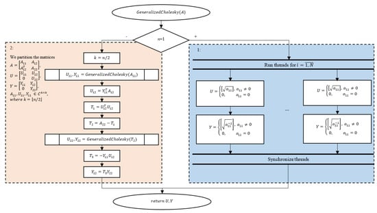
Figure 5.
Step 1 of Cholesky factorization for CUDA.
5.4. Strassen’s Matrix Inversion Algorithm
The implementation follows the block diagram given in Algorithm 4.2 (Figure 2). In case n = 1, we call a specialized kernel and proceed with the algorithm using recursive function calls and matrix multiplications (Figure 6). As before, we need to partition the matrices, create the temporary matrices, and manage their memory. The listing shows the implementation of Strassen’s matrix inversion algorithm [44]. We also use the auxiliary class StreamManager, which manages the CUDA streams.
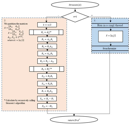
Figure 6.
Step 1 of Strassen’s matrix inverse algorithm: CUDA version.
In addition to using the GPU for matrix multiplications, we can also speed up the algorithm by utilizing parallelism on a higher level and exploiting the independence of some matrix multiplications. All the GPU operations in the strassen_matrix_inversion() function are executed by one of the two CUDA streams (note that the matmul function, as the last two arguments, has a stream and sync). After calculating the inverse matrix, we need to free the memory used for the intermediate results.
5.5. Calculating the Pseudoinverse
Finally, after presenting the algorithms for matrix multiplication [44], the generalized Cholesky factorization (Appendix A, Figure A1), and Strassen’s matrix inversion (Appendix A, Figure A2), we use these functions (based on Algorithm 4.3) to calculate the Moore–Penrose generalized inverse of an arbitrary real matrix. This main algorithm is run on the CPU. The pseudocode shows the code of a function that calculates and returns the pseudoinverse of an arbitrary matrix A passed as an argument to the function (Appendix A, Figure A3).
6. Computational Experiment and Analysis
To test the efficiency gained by using the GPU algorithm described in this paper, we measured and compared the execution time of the parallel algorithm from Section 5 that runs on the GPU and the serial algorithm that runs on the CPU (we used the cuBLAS library for matrix multiplication on the CPU). We also compared our implementation with the algorithm that uses the SVD to calculate the pseudoinverse: we used the algorithm from the OpenCV library (v.4.5.5, Intel Corporation, Santa Clara, USA) [46], which is executed solely on the CPU, and the algorithm from the PyTorch library (Linux Foundation, San Francisco, CA, USA) [47], which uses the GPU and CUDA internally. We compared the results for matrices of various shapes and both single and double precision.
Table 1 and Table 2 show the average time in milliseconds needed for calculating the Moore–Penrose generalized inverse for the float and double matrices, respectively, using the different algorithms and computing architectures. The OpenCV and PyTorch implementations are labeled as CPU-SVD and GPU-SVD, respectively. The recursive algorithm discussed in Section 5 is labeled as R and for the execution on the GPU, we measured the execution time of the algorithm that uses a custom matmul kernel (GPU-R-v1) and the algorithm where matrix multiplication is performed using the cuBLAS library (GPU-R-v2). The values in the table represent the mean of five measurements.

Table 1.
Time in milliseconds to calculate the pseudoinverse for float (single precision) matrices.
Table 2.
Time in milliseconds to calculate the pseudoinverse for double matrices.
Note that we measured only the time needed to calculate the pseudoinverse, not the time needed to transfer the memory between the CPU and GPU.
Figure 7 and Figure 8 show the data included in Table 1 and Table 2 for the float and double data types, respectively.
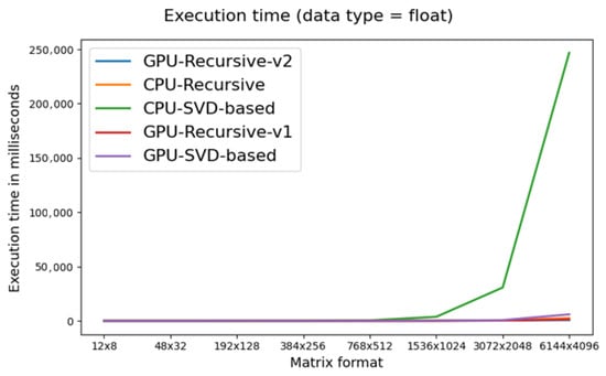
Figure 7.
Time in milliseconds to calculate the pseudoinverse of float matrix.
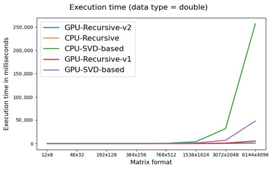
Figure 8.
Time in milliseconds to calculate the pseudoinverse of double matrix.
The tests were performed on a computer that has GeForce GTX 1080 Ti GPU, Intel(R) Core(TM) i7-9700 CPU 3.00 GHz (Santa Clara, CA, USA), and 16 GB of DDR4 ram memory (JEDEC, Arlington, VA, USA) (2400 MT/s speed). We used CUDA 11.7, cuBLAS 3.10, PyTorch 1.12.1 (with CUDA 10.2), and OpenCV 4.6.
It can be observed that the recursive implementation was faster than the SVD-based algorithm even when comparing CPU-R and GPU-SVD. The CPU implementations were notably faster for small matrices (with approximately less than 25,000 elements). For the larger matrices, we found that the CPU-R algorithm still outperformed GPU-SVD and was comparable to GPU-R-v1. However, when working with matrices with a few million elements (3072 × 2048), the implementation of matrix multiplication on the GPU becomes more important, especially in the case of double-precision multiplications, where GPU-R-v2 outperformed all the other algorithms. This gap further increased when working with even larger matrices (6144 × 4096). When working with single precision, the GPU-R1 implementation was 2 times faster than the same algorithm run on the CPU and 4.3 times faster than the SVD-based algorithm that runs on the GPU. When we used cuBLAS to perform matrix multiplication (GPU-R-v2), we obtained 2 times faster execution (4 times faster than CPU-R and 8.6 faster than GPU-SVD).
In the case of double-precision multiplication, we found the matrix multiplication algorithm on the GPU to be very important. While the recursive implementation still outperformed the SVD-based implementation (both on the CPU and GPU), CPU-R performed slightly better (for large matrices) than GPU-R-v1. When we used cuBLAS, the recursive GPU algorithm (GPU-R-v2) outperformed CPU-R up to 5 times and GPU-SVD up to 42 times.
If we compare CPU-SVD to GPU-R algorithms, a speedup of up to 342 times can be achieved (see Table 1 and results for a 6144 × 4096 matrix).
We can also see that the recursive algorithm described in this paper is more scalable than the traditional SVD approach and that the GPU implementation provides even better scalability than the CPU implementation of the same algorithm, especially if we use cuBLAS to multiply the matrices.
7. Conclusions
In our work, we introduced the recursive algorithm for the Moore–Penrose generalized inverse based on the algorithm by Petković and Stanimirović [28] for massively parallel systems with CUDA architecture to perform calculations on graphical processing units. Testing and comparing our parallel algorithm with the CPU implementation from the OpenCV library revealed the significant advantages of using the GPU for large matrices (with millions of elements and more). A speedup of up to 176 times was achieved compared with the (optimized) algorithm running on the CPU.
The Moore–Penrose inverse of some matrices that appear in graph theory has been frequently investigated. The main results refer to the Laplacian matrix [48], the Euclidean distance matrix [49,50], or the distance matrix [51]. The adaptation of the described algorithm to the matrices that appear in graph theory and their application can be the subject of future research.
Author Contributions
Conceptualization, P.S.S., L.K. and V.S.; methodology, P.S.S., L.K. and V.S.; software, V.S.; validation, V.S., G.S. and N.R.; formal analysis, P.S.S., L.K. and N.R.; investigation, V.S. and G.S.; resources, P.S.S.; data curation, V.S. and G.S.; writing—original draft preparation, G.S., V.S. and N.R.; writing—review and editing, V.S., L.K. and N.R.; visualization, V.S. and N.R.; supervision, P.S.S.; project administration, P.S.S.; funding acquisition, P.S.S. All authors have read and agreed to the published version of the manuscript.
Funding
This research was funded by the Ministry of Science and Higher Education of the Russian Federation, Grant No. 075-15-2022-1121.
Conflicts of Interest
The authors declare no conflict of interest.
Appendix A

Figure A1.
Generalized Cholesky factorization: CUDA implementation.


Figure A2.
Strassen’s matrix inversion algorithm: CUDA implementation.


Figure A3.
Calculating the pseudoinverse of an arbitrary real matrix.

References
- Wang, G.; Wei, Y.; Qiao, S. Generalized Inverses: Theory and Computations; Science Press: Beijing, China, 2018. [Google Scholar] [CrossRef]
- Golub, G.H.; Van Loan, C.F. Matrix Computations, 3rd ed.; The Johns Hopkins University Press: Baltimore, MD, USA, 1996. [Google Scholar]
- Stanimirović, P.S.; Mosić, D.; Wei, Y. Least squares properties of generalized inverses. Commun. Math. Res. 2021, 37, 421–447. [Google Scholar]
- Leiva, H.; Manzanilla, R. Moore-Penrose Inverse and Semilinear Equations. Adv. Linear Algebra Matrix Theory 2018, 8, 11–17. [Google Scholar] [CrossRef][Green Version]
- Bouman, N.J.; de Vreede, N. A Practical approach to the secure computation of the Moore-Penrose pseudoinverse over the rationals. IACR Cryptol. Eprint Arch. 2019, 2019, 470. [Google Scholar]
- Bozzo, E. The Moore–Penrose inverse of the normalized graph Laplacian. Linear Algebra Its Appl. 2013, 439, 3038–3043. [Google Scholar] [CrossRef]
- Azimi, A.; Bapat, R.B. Moore–Penrose inverse of the incidence matrix of a distance regular graph. Linear Algebra Its Appl. 2018, 551, 92–103. [Google Scholar] [CrossRef]
- Azimi, A.; Bapat, R. The Moore–Penrose inverse of the incidence matrix of complete multipartite and bi-block graphs. Discret. Math. 2019, 342, 2393–2401. [Google Scholar] [CrossRef]
- Azimi, A.; Bapat, R.B.; Estaji, E. Moore–Penrose inverse of incidence matrix of graphs with complete and cyclic blocks. Discret. Math. 2019, 342, 10–17. [Google Scholar] [CrossRef]
- Hessert, R.; Mallik, S. Moore-Penrose inverses of the signless Laplacian and edge-Laplacian of graphs. Discret. Math. 2021, 344, 112451. [Google Scholar] [CrossRef]
- Dang, V.H.; Nguyen, T.D. Construction of Pseudoinverse Matrix Over Finite Field and Its Applications. Wirel. Pers. Commun. 2017, 94, 455–466. [Google Scholar] [CrossRef]
- Kirichenko, N.F.; Lepekha, N.P. Application of Pseudoinverse and Projective Matrices to Studying Control, Observation, and Identification Problems. Cybern. Syst. Anal. 2002, 38, 568–585. [Google Scholar] [CrossRef]
- Chountasis, S.; Katsikis, V.N.; Pappas, D. Applications of the Moore-Penrose Inverse in Digital Image Restoration. Math. Probl. Eng. 2009, 2009, 170724. [Google Scholar] [CrossRef]
- Miljkovic, S.; Miladinovic, M.; Stanimirovic, P.; Stojanovic, I. Application of the pseudoinverse computation in reconstruction of blurred images. Filomat 2013, 26, 453–465. [Google Scholar] [CrossRef]
- Jurgen, R. 2001-01-0562 On-Line State Prediction of Engines Based on Fast Neural Network. In Electronic Engine Control Technologies; SAE: Sydney, Australia, 2004; pp. 713–719. [Google Scholar] [CrossRef]
- Huang, Y.; Huang, N.; Li, Y.; Shi, Y. Automated Fault Detection and Diagnosis for an Air Handling Unit Based on a GA-Trained RBF Network. In Proceedings of the 2006 International Conference on Communications, Circuits and Systems, Guilin, China, 25–28 June 2006; Volume 3, pp. 2038–2041. [Google Scholar] [CrossRef]
- Lima dos Reis Marques, F.; Floridia, C.; Alves Almeida, T.; Leonardi, A.A.; Fruett, F. Separation of temperature and strain in a single fiber BOTDA system by pseudo-inverse approach. In Proceedings of the 2017 SBMO/IEEE MTT-S International Microwave and Optoelectronics Conference (IMOC), Aguas de Lindoia, Brazil, 27–30 August 2017; pp. 1–4. [Google Scholar] [CrossRef]
- Corbella, I.; Torres, F.; Camps, A.; Duffo, N.; Vall-Llossera, M. Brightness-Temperature Retrieval Methods in Synthetic Aperture Radiometers. IEEE Trans. Geosci. Remote Sens. 2009, 47, 285–294. [Google Scholar] [CrossRef]
- Tapson, J.; van Schaik, A. Learning the pseudoinverse solution to network weights. Neural Netw. 2013, 45, 94–100. [Google Scholar] [CrossRef]
- Sevinov, J. Regularized Algorithms for the Formation of Control Actions in Locally Optimal Control Systems for Dynamic Objects. Int. J. Adv. Res. Sci. Eng. Technol. 2018, 5, 5853–5857. [Google Scholar]
- Jin, L.; Zhang, Y. Discrete-time Zhang neural network of O(τ3) pattern for time-varying matrix pseudoinversion with application to manipulator motion generation. Neurocomputing 2014, 142, 165–173. [Google Scholar] [CrossRef]
- Hu, Z.; Xiao, L.; Li, K.; Li, K.; Li, J. Performance analysis of nonlinear activated zeroing neural networks for time-varying matrix pseudoinversion with application. Appl. Soft Comput. 2021, 98, 106735. [Google Scholar] [CrossRef]
- Tanabe, K. Neumann-type expansion of reflexive generalized inverses of a matrix and the hyperpower iterative method. Linear Algebra Its Appl. 1975, 10, 163–175. [Google Scholar] [CrossRef][Green Version]
- Pan, V.; Schreiber, R. An Improved Newton Iteration for the Generalized Inverse of a Matrix, with Applications. SIAM J. Sci. Stat. Comput. 1991, 12, 1109–1130. [Google Scholar] [CrossRef]
- Weiguo, L.; Juan, L.; Tiantian, Q. A family of iterative methods for computing Moore–Penrose inverse of a matrix. Linear Algebra Its Appl. 2013, 438, 47–56. [Google Scholar] [CrossRef]
- Liu, X.; Jin, H.; Yu, Y. Higher-order convergent iterative method for computing the generalized inverse and its application to Toeplitz matrices. Linear Algebra Its Appl. 2013, 439, 1635–1650. [Google Scholar] [CrossRef]
- Soleymani, F. An efficient and stable Newton-type iterative method for computing generalized inverse . Numer. Algorithms 2015, 69, 569–578. [Google Scholar] [CrossRef]
- Petković, M.D.; Stanimirović, P.S. Generalized matrix inversion is not harder than matrix multiplication. J. Comput. Appl. Math. 2009, 230, 270–282. [Google Scholar] [CrossRef]
- Chen, X.; Ji, J. Computing the Moore-Penrose Inverse of a Matrix through Symmetric Rank-One Updates. Am. J. Comput. Math. 2011, 1, 147–151. [Google Scholar] [CrossRef][Green Version]
- Kadiam, S.C. Sciences Applications: Research and Education. Ph.D. Dissertation, Civil & Environmental Engineering, Old Dominion University, Norfolk, VA, USA, 2012. [Google Scholar] [CrossRef]
- Yanai, H.; Takeuchi, K.; Takane, Y. Projection Matrices, Generalized Inverse Matrices, and Singular Value Decomposition; Springer: New York, NY, USA, 2011. [Google Scholar]
- Sun, W.; Wei, Y. Inverse Order Rule for Weighted Generalized Inverse. SIAM J. Matrix Anal. Appl. 1998, 19, 772–775. [Google Scholar] [CrossRef]
- Stanimirović, P.S.; Pappas, D.; Katsikis, V.N.; Stanimirović, I. Full–rank representations of outer inverses based on the QR decomposition. Appl. Math. Comput. 2012, 218, 10321–10333. [Google Scholar] [CrossRef]
- Andrilli, S.; David Hecker, D. Elementary Linear Algebra, 4th ed.; Academic Press: New York, NY, USA, 2009; 768p. [Google Scholar]
- Sheng, X.; Chen, G.L.; Gong, Y. The representation and computation of generalized inverse . J. Comput. Appl. Math. 2008, 213, 248–257. [Google Scholar] [CrossRef]
- Sheng, X.; Chen, G.L. A note of computation for M-P inverse A. Int. J. Comput. Math. 2010, 87, 2235–2241. [Google Scholar] [CrossRef]
- Ji, J. Gauss–Jordan elimination methods for the Moore–Penrose inverse of a matrix. Linear Algebra Its Appl. 2012, 437, 1835–1844. [Google Scholar] [CrossRef]
- Strang, G. Introduction to Linear Algebra, 5th ed.; Wellesley-Cambridge Press: Wellesley, MA, USA, 2016; 600p. [Google Scholar]
- Penrose, R. A generalized inverse for matrices. Math. Proc. Camb. Philos. Soc. 1955, 51, 406–413. [Google Scholar] [CrossRef]
- Soyata, T. GPU Parallel Program Development Using CUDA, 1st ed.; Chapman and Hall/CRC: New York, NY, USA, 2018. [Google Scholar] [CrossRef]
- Strassen, V. Gaussian elimination is not optimal. Numer. Math. 1969, 13, 354–356. [Google Scholar] [CrossRef]
- Courrieu, P. Straight monotonic embedding of data sets in Euclidean spaces. Neural Netw. 2002, 15, 1185–1196. [Google Scholar] [CrossRef]
- Courrieu, P. Fast solving of weighted pairing least-squares systems. J. Comput. Appl. Math. 2009, 231, 39–48. [Google Scholar] [CrossRef][Green Version]
- Stanojević, V.; Kazakovtsev, L.; Stanimirović, P.S.; Rezova, N.; Shkaberina, G. Program Code for Calculating Moore-Penrose Generalized Inverse on Massive-Parallel Systems. Available online: http://levk.info/GPUMoorePenroseCode.zip (accessed on 28 August 2022).
- Higham, N.J. Cholesky factorization. Wiley Interdiscip. Rev. Comput. Stat. 2009, 1, 251–254. [Google Scholar] [CrossRef]
- OpenCV Team. Available online: https://www.google-melange.com/archive/gsoc/2014/orgs/opencv (accessed on 28 August 2022).
- PyTorch Library. Available online: http://citebay.com/how-to-cite/pytorch (accessed on 28 August 2022).
- Gutman, I.; Xiao, W. Generalized inverse of the Laplacian matrix and some applications. Bull. Cl. Sci. Math. Natturalles 2004, 129, 15–23. [Google Scholar] [CrossRef]
- Kurata, H.; Bapat, R.B. Moore–Penrose inverse of a Euclidean distance matrix. Linear Algebra Its Appl. 2015, 472, 106–117. [Google Scholar] [CrossRef]
- Balaji, R.; Bapat, R.B. On Euclidean distance matrices. Linear Algebra Its Appl. 2007, 424, 108–117. [Google Scholar] [CrossRef]
- Jeyaraman, I.; Divyadevi, T.; Azhagendran, R. The Moore-Penrose Inverse of the Distance Matrix of a Helm Graph. arXiv 2022, arXiv:2208.10897. [Google Scholar] [CrossRef]


Publisher’s Note: MDPI stays neutral with regard to jurisdictional claims in published maps and institutional affiliations. |
© 2022 by the authors. Licensee MDPI, Basel, Switzerland. This article is an open access article distributed under the terms and conditions of the Creative Commons Attribution (CC BY) license (https://creativecommons.org/licenses/by/4.0/).