
Mixed Poisson Regression Models with Varying Dispersion Arising from Non-Conjugate Mixing Distributions


Abstract
:1. Introduction
2. Mixed Poisson Regression Model with Varying Dispersion
2.1. Modelling Framework
2.2. Model Specification: The Poisson-Lognormal Regression Model with Varying Dispersion
3. Statistical Inference: The EM-Type Algorithm
- E-Step: The Q-function, which is the conditional expectation of the complete data log-likelihood, is given bywhere is the estimate of at the rth iteration in the E-step of our EM algorithm. Then, using the estimates , calculate the pseudo-values and for and , where are certain functions which are involved in the terms needed for maximizing the part of the Q-function which corresponds to the conditional expectation of the log-likelihood of the mixing distribution .
- M-Step: Using the pseudo-values and from the E-Step and the Newton–Raphson algorithm twice, find the maximum global point of the Q-function, that is, obtain the updated estimates and .
- -
- Firstly, taking the necessary derivatives of the Q-function with respect to , we obtain the following resultsandfor and , and whereThen, the iterative procedure for the Newton–Raphson algorithm for goes as follows
- -
- Secondly, differentiating the Q-function with respect to givesandwhere for computing and , we need to use the pseudo-values for and , because in this case, the maximization of the Q-function reduces to the maximization of the conditional expectation of the log-likelihood of the mixing distribution .Then, the Newton–Raphson iterative algorithm for is as followsfor and .
- Finally, iterate between the E- and the M-Steps until some convergence criterion is satisfied, for instancewhere is the value of the log-likelihood after the r-th iteration, and where is a small number usually of the form , where The stopping criterion refers to the progress of the likelihood function (i.e., its convergence). If the stopping criterion is satisfied, the EM algorithm stops iterating, and the estimate of is . Otherwise, is updated by , and the algorithm returns to the E-step.
EM Estimation for the PLN Regression Model with Varying Dispersion
| Algorithm 1 EM Algorithm for the PLN Regression Model with Varying Dispersion |
|
- E-Step:Calculate, for all ,andwhere and .Note that the expectations in Equations (24) and (25) can be evaluated numerically. Alternatively, a Monte Carlo approach can be used based on a rejection algorithm, leading to variants of the EM algorithm, such as the Monte Carlo EM (MCEM) algorithm, which do not rely on the pdf , that cannot be written in closed form, but it is sufficent to simulate from the posterior distribution
- M-Step:
- -
- -
- Secondly, the regression parameters are updated using the pseudo-values and , which are given by Equations (24) and (25), respectively, and the Newton–Raphson algorithm, which, in the case of the lognormal mixing distribution, is as followsandfor and , and whereThen, we can obtain the updated estimates of as follows
4. Numerical Illustration
- The NBI regression model with varying dispersion is derived as follows. Consider policyholder i, , whose number of claims, denoted as , with , are independent. In addition, assume that follows a Poisson distribution with pmf given by Equation (1), and follows a Gamma distribution with pdf given bywhere . Parameterization (29) ensures that , and hence the model is identifiable.Then, the unconditional distribution of becomes an NBI distribution, with pmf given byThe mean and the variance of the NBI distribution are given byand
- The mean and dispersion parameters of the NBI distribution are modelled in terms of covariateswhere and are covariate vectors with dimensions and , respectively, with and the corresponding parameter vectors, and where it is assumed that the matrices and with rows given by and , respectively, are of full rank.
- The pmf of the ZIP regression model is given byThe mean and the variance of the ZIP distribution are given byandwhere , and where is a covariate vector with dimension , with the corresponding parameter vector, and where it is assumed that the matrix with rows given by , respectively, are of full rank (note that can also be modelled in terms of covariates using the logit link function. However, we refrain from doing this in this paper since this approach did not lead to better fitting performances for the ZIP model for the MTPL data).
4.1. Modelling Results
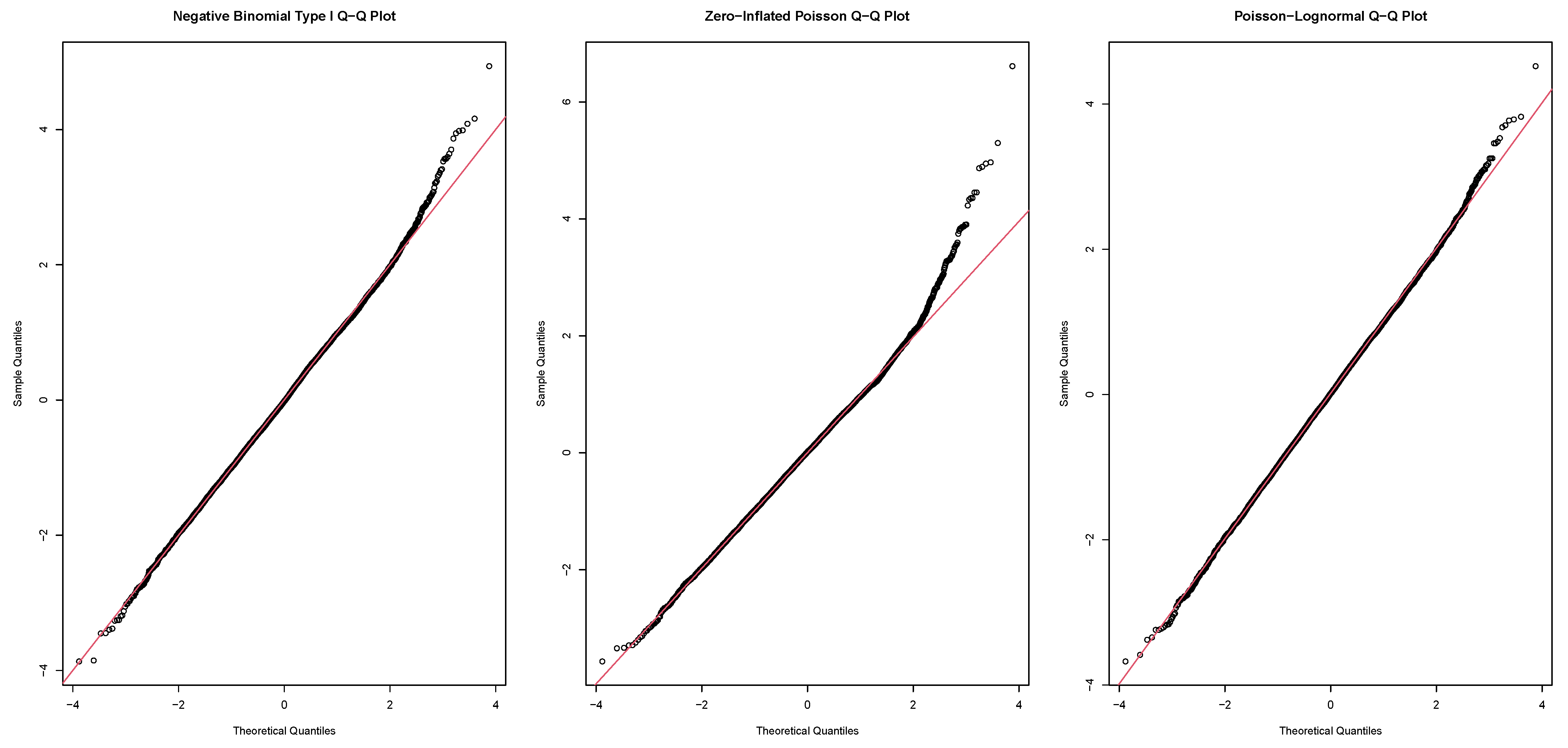
4.2. Models Comparison
4.3. Computational Aspects
5. Conclusions, Limitations, and Future Research
Author Contributions
Funding
Institutional Review Board Statement
Informed Consent Statement
Data Availability Statement
Acknowledgments
Conflicts of Interest
Abbreviations
| EM | Expectation-maximization |
| NBI | Negative binomial type I |
| MCEM | Monte Carlo expectation-maximization |
| ML | Maximum likelihood |
| MTPL | Motor third-party liability |
| Probability density function | |
| PLN | Poisson log-normal |
| pmf | Probability mass function |
| ZIP | Zero-inflated Poisson |
References
- Lawless, J.F. Negative binomial and mixed Poisson regression. Can. J. Stat. 1987, 15, 209–225. [Google Scholar] [CrossRef]
- Cameron, A.C.; Trivedi, P.K. Regression Analysis of Count Data, 1st ed.; Cambridge University Press: Cambridge, UK, 1998. [Google Scholar]
- Hilbe, J.M. Negative Binomial Regression, 1st ed.; Cambridge University Press: Cambridge, UK, 2008. [Google Scholar]
- Ord, J.K.; Whitmore, G.A. The Poisson-inverse Gaussian distribution as a model for species abundance. Commun. Stat. Theory Methods 1986, 15, 853–871. [Google Scholar] [CrossRef]
- Willmot, G.E. The Poisson-Inverse Gaussian distribution as an alternative to the negative binomial. Scand. Actuar. J. 1987, 3–4, 113–127. [Google Scholar] [CrossRef]
- Dean, C.; Lawless, J.F.; Willmot, G.E. A mixed Poisson–inverse-Gaussian regression model. Can. J. Stat. 1989, 17, 171–181. [Google Scholar] [CrossRef]
- Perline, R. Mixed Poisson distributions tail equivalent to their mixing distributions. Stat. Comput. 1998, 38, 229–233. [Google Scholar] [CrossRef]
- Rigby, R.A.; Stasinopoulos, D.M.; Akantziliotou, C. A framework for modelling overdispersed count data, including the Poisson-shifted generalized inverse Gaussian distribution. Comput. Stat. Data Anal. 2008, 53, 381–393. [Google Scholar] [CrossRef]
- Barreto-Souza, W.; Simas, A.B. General mixed Poisson regression models with varying dispersion. Stat. Comput. 2016, 26, 1263–1280. [Google Scholar] [CrossRef]
- Tzougas, G. EM estimation for the Poisson–inverse Gamma regression model with varying dispersion: An application to insurance ratemaking. Risks 2020, 8, 97. [Google Scholar] [CrossRef]
- Blueschke, D.; Blueschke-Nikolaeva, V.; Neck, R. Approximately Optimal Control of Nonlinear Dynamic Stochastic Problems with Learning: The OPTCON Algorithm. Algorithms 2021, 14, 181. [Google Scholar] [CrossRef]
- Amirghasemi, M. An Effective Decomposition-Based Stochastic Algorithm for Solving the Permutation Flow-Shop Scheduling Problem. Algorithms 2021, 14, 112. [Google Scholar] [CrossRef]
- Dunn, P.K.; Smyth, G.K. Randomized quantile residuals. Comput. Graph. Stat. 1996, 5, 236–245. [Google Scholar]
- Stasinopoulos, D.M.; Rigby, B.; Akantziliotou, C. Instructions on How to Use the Gamlss Package in R, 2nd ed. 2008. Available online: http://www.gamlss.org (accessed on 30 December 2021).
- Louis, T.A. Finding the observed information matrix when using the EM algorithm. J. R. Stat. Soc. 1982, 44, 226–233. [Google Scholar]

| Statistic | Value | Age of the Driver (AD) | Horsepower of the Car (HP) | Age of the Car (AC) | |||
|---|---|---|---|---|---|---|---|
| # Observations | 14,143 | C1: | 3238 | C1: | 5042 | C1: | 4318 |
| Minimum | 0 | C2: | 10,905 | C2: | 9101 | C2: | 9825 |
| Median | 0 | - | - | - | |||
| Mean | 0.4827 | - | - | - | |||
| Variance | 0.6988 | - | - | - | |||
| Maximum | 12 | - | - | - | |||
| NBI | ZIP | PLN | |||
|---|---|---|---|---|---|
| Coeff. | Coeff. | Coeff. | |||
| Intercept | Intercept | Intercept | |||
| AD | CS | CS | |||
| C2 | C2 | C2 | |||
| HP | HP | HP | |||
| C2 | C2 | C2 | |||
| AC | AC | AC | |||
| C2 | C2 | C2 | |||
| Coeff. | Coeff. | ||||
| Intercept | Prob. | Intercept | |||
| AD | CS | ||||
| C2 | C2 | ||||
| Specification Criteria Values | |||
|---|---|---|---|
| DEV | AIC | SBC | |
| NBI | 15,885.1 | 15,897.1 | 15,940.1 |
| ZIP | 16,052.2 | 16,062.2 | 16,098 |
| PLN | 15,859.4 | 15,871.4 | 15,914.4 |
Publisher’s Note: MDPI stays neutral with regard to jurisdictional claims in published maps and institutional affiliations. |
© 2021 by the authors. Licensee MDPI, Basel, Switzerland. This article is an open access article distributed under the terms and conditions of the Creative Commons Attribution (CC BY) license (https://creativecommons.org/licenses/by/4.0/).
Share and Cite
Tzougas, G.; Hong, N.; Ho, R. Mixed Poisson Regression Models with Varying Dispersion Arising from Non-Conjugate Mixing Distributions. Algorithms 2022, 15, 16. https://doi.org/10.3390/a15010016
Tzougas G, Hong N, Ho R. Mixed Poisson Regression Models with Varying Dispersion Arising from Non-Conjugate Mixing Distributions. Algorithms. 2022; 15(1):16. https://doi.org/10.3390/a15010016
Chicago/Turabian StyleTzougas, George, Natalia Hong, and Ryan Ho. 2022. "Mixed Poisson Regression Models with Varying Dispersion Arising from Non-Conjugate Mixing Distributions" Algorithms 15, no. 1: 16. https://doi.org/10.3390/a15010016
APA StyleTzougas, G., Hong, N., & Ho, R. (2022). Mixed Poisson Regression Models with Varying Dispersion Arising from Non-Conjugate Mixing Distributions. Algorithms, 15(1), 16. https://doi.org/10.3390/a15010016