On Parameter Identification for Reaction-Dominated Pore-Scale Reactive Transport Using Modified Bee Colony Algorithm

Abstract

Parameter identification is an important research topic with a variety of applications in industrial and environmental problems. Usually, a functional has to be minimized in conjunction with parameter identification; thus, there is a certain similarity between the parameter identification and optimization. A number of rigorous and efficient algorithms for optimization problems were developed in recent decades for the case of a convex functional. In the case of a non-convex functional, the metaheuristic algorithms dominate. This paper discusses an optimization method called modified bee colony algorithm (MBC), which is a modification of the standard bees algorithm (SBA). The SBA is inspired by a particular intelligent behavior of honeybee swarms. The algorithm is adapted for the parameter identification of reaction-dominated pore-scale transport when a non-convex functional has to be minimized. The algorithm is first checked by solving a few benchmark problems, namely finding the minima for Shekel, Rosenbrock, Himmelblau and Rastrigin functions. A statistical analysis was carried out to compare the performance of MBC with the SBA and the artificial bee colony (ABC) algorithm. Next, MBC is applied to identify the three parameters in the Langmuir isotherm, which is used to describe the considered reaction. Here, 2D periodic porous media were considered. The simulation results show that the MBC algorithm can be successfully used for identifying admissible sets for the reaction parameters in reaction-dominated transport characterized by low Pecklet and high Damkholer numbers. Finite element approximation in space and implicit time discretization are exploited to solve the direct problem.

1. Introduction

Reactive transport in porous media is an important component of many industrial and environmental problems. Historically, most of the theoretical and experimental research on transport in porous media in general, and reactive transport in particular, has been carried out at the macroscopic Darcy scale [1,2]. In many cases, the bottleneck in performing computational modeling of reactive transport is the absence of data for the pore-scale adsorption and desorption rate (or in more general terms, the parameters of the heterogeneous reactions). Despite the progress in developing devices to perform experimental measurements at the pore scale, experimental characterization of these rates is still a complex and expensive process.

In the case of heterogeneous reactions at the pore scale, the species transport is coupled to surface reaction via boundary conditions. When the reaction rates are not known, their identification falls into the class of boundary value inverse problems [3,4,5,6]. The additional information which is needed to identify the parameters is often provided in the form of the dynamic change of the concentration at the outlet (e.g., so-called breakthrough curves). In the literature, inverse problems in porous media flow are discussed mainly in connection with parameter identification for macroscopic, Darcy-scale problems. An overview on inverse problems in groundwater Darcy-scale modeling can be found in [7]. The identification of parameters for pore-scale models is discussed in this paper, and the algorithms from [7] and other papers discussing parameter identification at the macro scale cannot be applied here without modification. Let us shortly mention some general approaches for solving inverse problems.

Different algorithms can be applied for solving parameter identification problems, see, e.g., [8,9]. Many of these algorithms exploit deterministic methods based on Tikhonov regularization technique [10,11] and target minimizing a functional of the difference between measured and computed quantities. An important part of such algorithms is the definition of a feasible set of parameters on which the functional is minimized. Local or global optimization procedures are used in the optimization [12,13]. In this sense, it could be observed that there is a certain similarity between the mathematical formulation of an optimization problem and of a parameter identification problem.

Metaheuristic methods are a relatively new and rapidly developing class of optimization methods. There are various metaheuristic algorithms: genetic algorithms (GA) [14], particle swarm optimization (PSO) [15], genetic programming (GP) [16], differential evolution (DE) [17], and greedy randomized adaptive search procedure (GRASP) [18], to name just a few.

Metaheuristic algorithms are the working horse in studying different and distinct applications. Some examples of recent works are as follows: DE and ABC algorithms were used to identify the kinetic parameters in CO2 hydrogenation for the production of hydrocarbons [19]; PSO was used to calibrate parameters of anaerobic digestion model [20]; and GRASP was used for post-disaster route prediction for a multi-period work-troops scheduling problem on the example of the city of Port-au-Prince in Haiti after the 2010 earthquake [21]. More information on metaheuristic algorithms can be found in [22,23,24,25].

Among metaheuristic methods, evolutionary and behavioral ones stand out. Behavioral methods are multi-agent methods based on modeling the intellectual behavior of agent colonies (swarm intelligence). Swarm intelligence has become a research interest of many scientists and practitioners in the last decades. The bees algorithm was proposed by Pham, Ghanbarzadeh et al. in 2005 [26,27]. It mimics the food foraging behaviour of honey bee colonies. Later, the algorithm was explored and discussed in [28,29,30]. An analysis of BA can be found in [31]. An overview of the major branches of the bee method was published in [32]. According to this overview, there is the basic bees algorithm (BBA), where local areas remain fixed; shrinking-based bees algorithm (ShBA), where local areas may shrink in the case of stagnation, and finally, standard bees algorithm (SBA), where, in addition to the shrinkage, there is also a procedure to abandon local areas under certain conditions.

The artificial bee colony (ABC) algorithm was introduced by Karaboga in 2005 [33]. More about this algorithm, including its performance and convergence, can be found in  [34,35]. An essential difference of the ABC algorithm from BA is that bees can leave their local area if there is not enough nectar. This can be very useful when looking for a global extremum: the algorithm can converge much faster. The undoubted advantage of these algorithms is that it can be generalized to problems of any dimension, and it can be easily be run in parallel on supercomputers.

In this work, the standard bees algorithm (SBA) is modified and adapted for identifying parameters for reaction-dominated pore-scale transport. The algorithm used here is called the modified bee colony (MBC) algorithm to distinguish it from the SBA. The MBC is adapted to specifics of the considered class of problems, which are characterized by the presence of a non-convex functional, having the shape of a narrow valley with steep banks (see the plots in Section 4). The peculiarities of MBC are discussed in more details in Section 4. MBC was implemented in Python together with the other tested methods.

The MBC algorithm is used to identify admissible sets of parameters in a Langmuir isotherm in the case of reaction-dominated transport. Note that the goal here is not to identify just a point in the parameter space but to identify sets (called admissible sets here) such that, for each point from an admissible set, the functional is smaller than a prescribed threshold. Such parameter identification problems are important in many industrial processes.

The remainder of the paper is organized as follows. Pore-scale reactive transport is considered in Section 2. At the pore scale, single phase laminar flow described by incompressible Stokes equations and solute transport described by a convection-diffusion equation are considered. The surface reaction is accounted for in the boundary conditions. Henry and Langmuir adsorption isotherms are considered [36]. Section 3 is dedicated to the description of the used computational algorithm. Finite element method is exploited after triangulation of the computational domain. The numerical investigation of the grid convergence and sensitivity with respect to parameters is also presented in this Section. A modified bee colony algorithm is described in detail in Section 4. The algorithm has been tested on benchmark functions, and a comparative statistical analysis between MBC, SBA and ABC for 100 independent runs is presented. A parameter identification problem for reaction-dominated pore-scale transport is described in Section 5. Finally, Section 6 summarizes the results presented in this paper.

2. Pore-Scale Reactive Transport

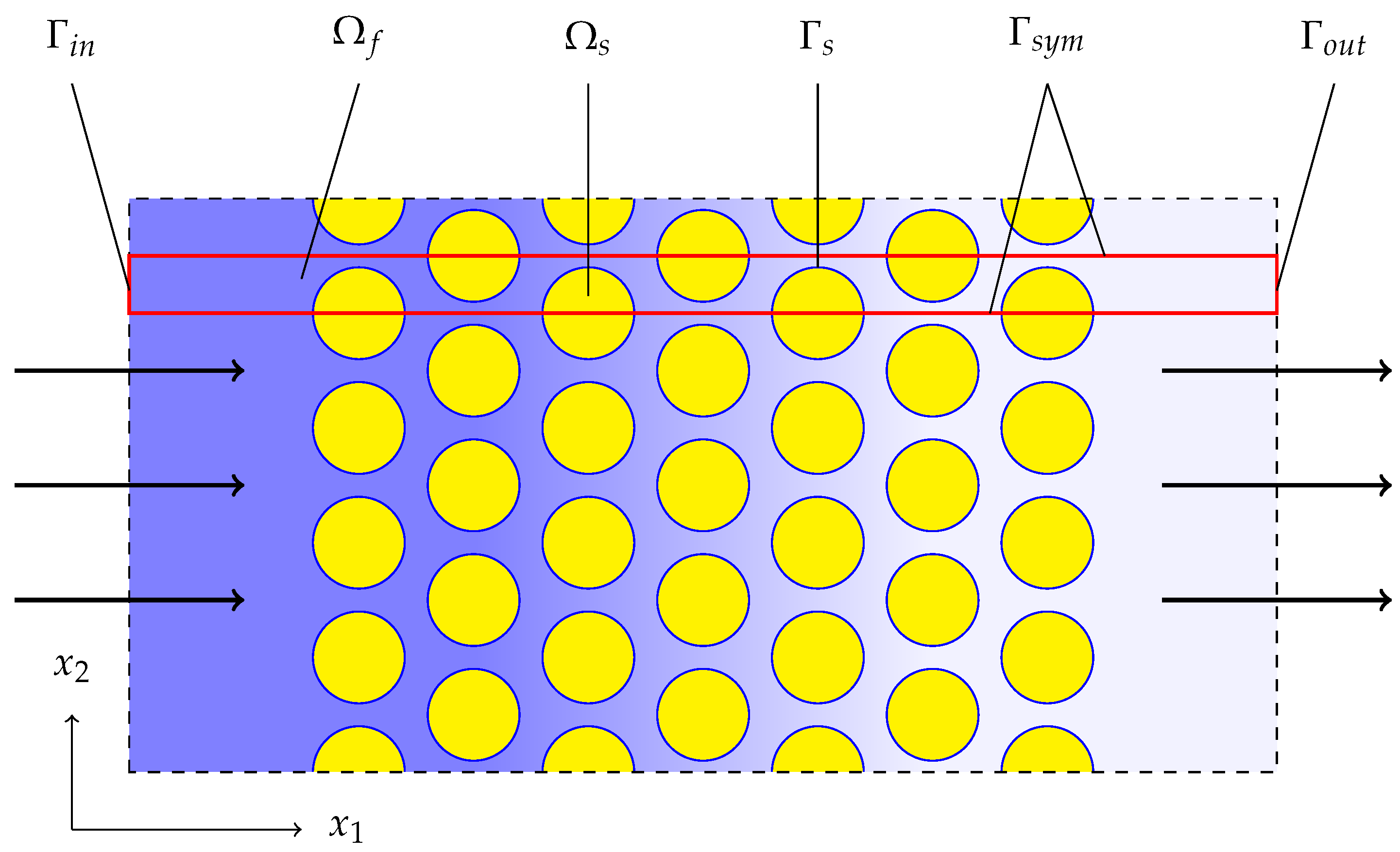
This work is one of a series of articles dedicated to parameter identification for pore-scale reactive flow. The same mathematical model is used in all cases, but different algorithms are explored. In the previous works [37,38], the diffusion-dominated case, characterised by small Damkhöler numbers, is investigated by means of stochastic and deterministic algorithms. In this work, we will deal with the reaction-dominated case, where the Damköler numbers are large, and in this situation, parameter identification process can be difficult. A metaheuristic algorithm is adapted in this study. For simplicity of analysis, we will consider the porous media as periodically arranged circles in the two-dimensional case. The scheme of the domain is shown on Figure 1. Due to the periodicity, we will only generate a computational grid from a segment of the entire domain, which is marked with a red rectangle on Figure 1. A part of the domain, namely ${\mathsf{\Omega }}_f$, is occupied by a fluid, while the other part is occupied by obstacles, which are denoted by ${\mathsf{\Omega }}_s$. The obstacle surfaces (where the reaction occurs) are denoted by ${\mathsf{\Gamma }}_s$, while symmetry lines are denoted by ${\mathsf{\Gamma }}_{sym}$. It is supposed that the dissolved substance is introduced via the inlet boundary ${\mathsf{\Gamma }}_{in}$, and the part of the substance which did not react flows out via ${\mathsf{\Gamma }}_{out}$. Since the adsorption reaction occurs only on the surface of obstacles, the computational domain consists only of ${\mathsf{\Omega }}_f$.

2.1. Flow Problem

The flow in the pores can be described here by the steady-state incompressible Stokes equations:

$$\nabla p-\mu {\nabla }^2\mathit{u}=0,$$

(1)

$$\nabla ·\mathit{u}=0,\mathit{x}\in {\mathsf{\Omega }}_f,t>0,$$

(2)

where $\mathit{u}\left(\mathit{x}\right)$ and $p\left(\mathit{x}\right)$ are the fluid velocity and pressure, respectively, while $\mu >0$ is the dynamic viscosity, which we assume to be constant and equal to 1 [1,39].

Denoting by $\mathit{n}$ the outer normal vector to the boundary, the suitable boundary conditions on $\partial {\mathsf{\Omega }}_f$ are specified as:

$$\mathit{u}·\mathit{n}=\overline{u},\mathit{u}\times \mathit{n}=0,\mathit{x}\in {\mathsf{\Gamma }}_{in},$$

(3)

$$p-\mathit{\sigma }\mathit{n}·\mathit{n}=\overline{p},\mathit{\sigma }\mathit{n}\times \mathit{n}=0,\mathit{x}\in {\mathsf{\Gamma }}_{out},$$

(4)

$$\mathit{u}·\mathit{n}=0,\mathit{u}\times \mathit{n}=0,\mathit{x}\in {\mathsf{\Gamma }}_s,$$

(5)

$$\mathit{u}·\mathit{n}=0,\mathit{\sigma }\mathit{n}\times \mathit{n}=0,\mathit{x}\in {\mathsf{\Gamma }}_{sim}.$$

(6)

The velocity of the fluid is 1 at the inlet, and at the outlet, the pressure and absence of the tangential force are prescribed. Standard no-slip and no-penetration conditions are prescribed on the solid walls, ${\mathsf{\Gamma }}_s$. Symmetry conditions are prescribed on the symmetry boundary of the computational domain ${\mathsf{\Gamma }}_{sym}$.

2.2. Species Transport

When a problem needs to be solved for a range of parameters (as is our goal here), working with the dimensionless form of the equations give definitive advantages. The height of the computational domain ${\mathsf{\Omega }}_f$, namely l, is used for scaling spatial sizes. The scaling of the velocity is done by the inlet velocity $\overline{u}$, and the scaling of the concentration is done by the inlet concentration $\overline{c}$. The concentration of the solute in the fluid is denoted by $c(\mathit{x},t)$. The unsteady solute transport under the conditions of heterogeneous reactions is governed by the convection-diffusion equation in its dimensionless form:

$$\frac{\partial c}{\partial t}+\nabla \left(\mathit{u}c\right)-\frac{1}{\mathrm{Pe}}{\nabla }^{2}c=0,\mathit{x}\in {\mathsf{\Omega }}_f,t>0,$$

(7)

where

$$\mathrm{Pe}=\frac{l\overline{u}}{D}$$

is the Peclet number. The boundary conditions are written as follows:

$$c=\overline{c},\mathit{x}\in {\mathsf{\Gamma }}_{in},$$

(8)

$$\nabla c·\mathit{n}=0,\mathit{x}\in {\mathsf{\Gamma }}_{sim}\cup {\mathsf{\Gamma }}_{out},$$

(9)

$$\frac{\partial m}{\partial t}=-\nabla c·\mathit{n},\mathit{x}\in {\mathsf{\Gamma }}_s.$$

(10)

The concentration of the solute at the inlet is assumed to be known. Zero diffusive flux of the solute at the outlet and on the external boundaries of the domain is prescribed. Note that convective flux via the outlet is implicitly allowed by the above equations. The surface reactions that occur at the obstacles’ surface, ${\mathsf{\Gamma }}_s$, satisfy the mass conservation law, in this particular case meaning that the change in the adsorbed surface concentration is equal to the flux from the fluid to the surface (10), where m is the surface concentration of the adsorbed solute [36].

A mixed kinetic–diffusion adsorption description is used:

$$\frac{\partial m}{\partial t}=f(c,m).$$

(11)

For reactive boundaries, the choice of f and its dependence on c and m are critical for a correct description of the reaction dynamics at the solid–fluid interface. A number of different isotherms (i.e., different functions $f(c,m)$) exist for describing these dynamics, which are dependent on the solute attributes, the order of the reaction, and the interface type.

The simplest of these is the Henry isotherm, which assumes a linear relationship between the near-surface concentration and the surface concentration of the adsorbed particles. In its dimensionless form, this is written as follows:

$$\frac{\partial m}{\partial t}={\mathrm{Da}}_{a}c-{\mathrm{Da}}_{d}m,\mathit{x}\in {\mathsf{\Gamma }}_s,$$

(12)

where the adsorption and desorption Damkoler numbers are given by

$${\mathrm{Da}}_a=\frac{k_a}{\overline{u}},{\mathrm{Da}}_d=\frac{k_{d}l}{\overline{u}}.$$

Here, $k_a\ge 0$ is the rate of adsorption, measured in unit length per unit time, and $k_d\ge 0$ is the rate of desorption, measured per unit time.

We used this isotherm in our previous work in our diffusion-dominated case investigation [37] and we will come back to it later when comparing the operation of the MBC algorithm in the penultimate section. In this work, we use the Langmuir adsorption isotherm, which is a more complicated three-parameter model:

$$\frac{\partial m}{\partial t}={\mathrm{Da}}_{a}c\left(1-\frac{m_{\infty }}{\mathrm{M}}\right)-{\mathrm{Da}}_{d}m,\mathit{x}\in {\mathsf{\Gamma }}_s,$$

(13)

where the dimensionless parameter M is given by

$$\mathrm{M}=\frac{m_{\infty }}{l\overline{c}}.$$

Here, $m_{\infty }>0$ is the maximal possible adsorbed surface concentration. In comparison to the Henry isotherm (12), the Langmuir isotherm (13) predicts a decrease in the rate of adsorption, as the adsorbed concentration increases due to the reduction in the available adsorption surface.

The formulation of the initial boundary value problem in addition to the governing Equations (1), (2) and (7), boundary conditions (3)–(6), (8)–(10), and specified isotherm (12) or (13) requires specification of the initial conditions:

$$c(\mathit{x},0)=0,\mathit{x}\in {\mathsf{\Omega }}_f.$$

(14)

$$m(\mathit{x},0)=0,\mathit{x}\in {\mathsf{\Gamma }}_s.$$

(15)

3. Numerical Simulation

Finite element method, FEM, is used for space discretization of the above problem, together with implicit discretization in time. The algorithm used here for solving the direct problem is practically identical to the algorithm used to study oxidation in [40].

3.1. Variational Formulation

Note that the fluid flow influences the species transport; however, the species concentration does not influence the fluid flow. Due to this, the flow can be computed only once in advance. The FEM approximation of the steady state flow problem [41] is based on the variational formulation of the considered boundary value problem (1)–(6). The following functional space $\mathit{V}$ is defined for the velocity $\mathit{u}$ ($\mathit{u}\in \mathit{V}$):

$$\begin{array}{cc}\hfill \mathit{V}=\{\mathit{u}\in {\mathit{H}}^1\left(\mathsf{\Omega }\right):& \mathit{u}·\mathit{n}=1,\mathit{u}\times \mathit{n}=0\mathrm{on}{\mathsf{\Gamma }}_{in},\hfill \\ & \mathit{u}=0\mathrm{on}{\mathsf{\Gamma }}_s,\mathit{u}·\mathit{n}=0\mathrm{on}{\mathsf{\Gamma }}_{sim}\}.\hfill \end{array}$$

Test function $\mathit{v}\in \widehat{\mathit{V}}$, where

$$\widehat{\mathit{V}}=\{\mathit{v}\in {\mathit{H}}^1\left({\mathsf{\Omega }}_f\right):\mathit{v}=0\mathrm{on}{\mathsf{\Gamma }}_{in},\mathit{v}=0\mathrm{on}{\mathsf{\Gamma }}_s,\mathit{v}·\mathit{n}=0\mathrm{on}{\mathsf{\Gamma }}_{sim}\}.$$

For the pressure p and the related test functions q, it is required that $p,q\in Q$, where

$$Q=\{q\in L_2\left({\mathsf{\Omega }}_f\right):q=0\mathrm{on}{\mathsf{\Gamma }}_{out}\}.$$

Multiplying (1) by $\mathit{v}$, (2) by q, integrating over the computational domain and taking into account the boundary conditions (3)–(6), the following system of equations is obtained with respect to $\mathit{v}\in \mathit{V}$, $p\in Q$:

$$a(\mathit{u},\mathit{v})-b(\mathit{v},p)=0\forall \mathit{v}\in \widehat{\mathit{V}},$$

(16)

$$b(\mathit{u},q)=0\forall q\in Q.$$

(17)

where

$$a(\mathit{u},\mathit{v}):={\int }_{{\mathsf{\Omega }}_f}\nabla \mathit{u}·\nabla \mathit{v}d\mathit{x},$$

$$b(\mathit{v},q):={\int }_{{\mathsf{\Omega }}_f}(\nabla ·\mathit{v})qd\mathit{x}.$$

The following finite dimensional subspaces are used for the basis and test functions in the FEM approximation of the velocity and the pressure: ${\mathit{V}}_h\subset \mathit{V}$, ${\widehat{\mathit{V}}}_h\subset \widehat{\mathit{V}}$ and $Q_h\subset Q$.

The unsteady species transport problem (7)–(10) is solved numerically using finite elements. Here we define

$$S=\{c\in H^1\left({\mathsf{\Omega }}_f\right):c=1\mathrm{on}{\mathsf{\Gamma }}_{in}\},$$

$$\widehat{S}=\{s\in H^1\left({\mathsf{\Omega }}_f\right):s=0\mathrm{on}{\mathsf{\Gamma }}_{in}\}.$$

The approximate solution $c\in S$ is sought from

$$\left(\frac{\partial c}{\partial t},s\right)+d(c,s)={\left(\frac{\partial m}{\partial t},s\right)}_s\forall s\in \widehat{S},$$

(18)

where the following notations are used:

$$d(c,s):=-{\int }_{{\mathsf{\Omega }}_f}c\mathit{u}·\nabla sd\mathit{x}+\frac{1}{\mathrm{Pe}}{\int }_{{\mathsf{\Omega }}_f}\nabla c·\nabla sd\mathit{x}+{\int }_{{\mathsf{\Gamma }}_{out}}(\mathit{u}·\mathit{n})csd\mathit{x},$$

$${(\phi ,s)}_s:=-{\int }_{{\mathsf{\Gamma }}_s}\phi sd\mathit{x}.$$

For determining $m\in G=L_2\left({\mathsf{\Gamma }}_s\right)$ (see (11)) we use

$${\left(\frac{\partial m}{\partial t},g\right)}_s-{(f(c,m),g)}_s=0,g\in G.$$

(19)

The symmetric Crank–Nicolson discretization method is used for time discretization. Let $\tau$ be a step-size of a uniform grid in time such that $c^n=c\left(t^n\right),t^n=n\tau ,n=0,1,\dots$.

Equation (18) is approximated in time as follows

$$\left(\frac{c^{n+1}-c^n}{\tau },s\right)+d\left(\frac{c^{n+1}+c^n}{2},s\right)={\left(\frac{m^{n+1}-m^n}{\tau },s\right)}_s.$$

In a similar way, for (19), we get

$${\left(\frac{m^{n+1}-m^n}{\tau },g\right)}_s-{\left(f\left(\frac{c^{n+1}+c^n}{2},\frac{m^{n+1}+m^n}{2}\right),g\right)}_s=0,n=0,1,\dots$$

We will not show pictures of the solution of the direct problem in this paper, since it differs from the previous work only by a length of time. This length was $T=40$, but is now $T=6000$, because this time, we are considering a case of a dominant reaction; therefore, the breakthrough curve looms over a long period of time. We have performed a direct solution to the problem on exactly the same geometry of the computational domain. Therefore, interested readers are encouraged to reference the computational fields in our previous work [37].

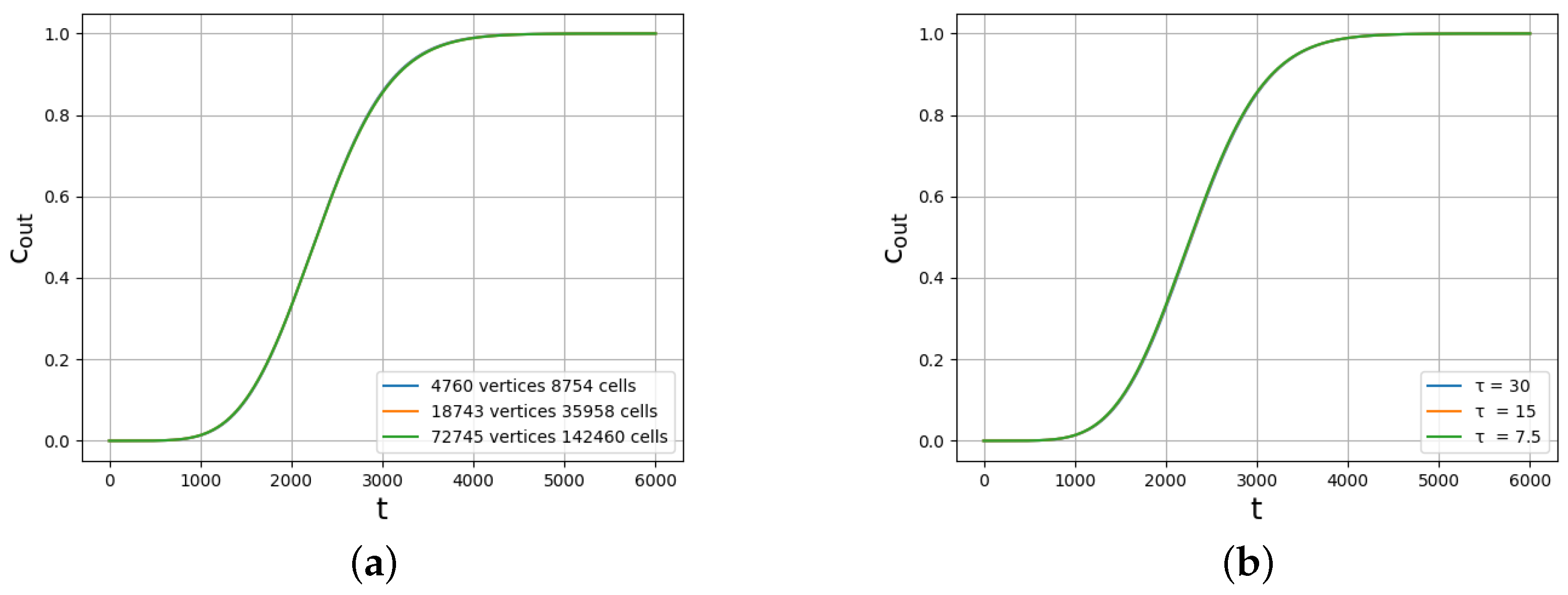
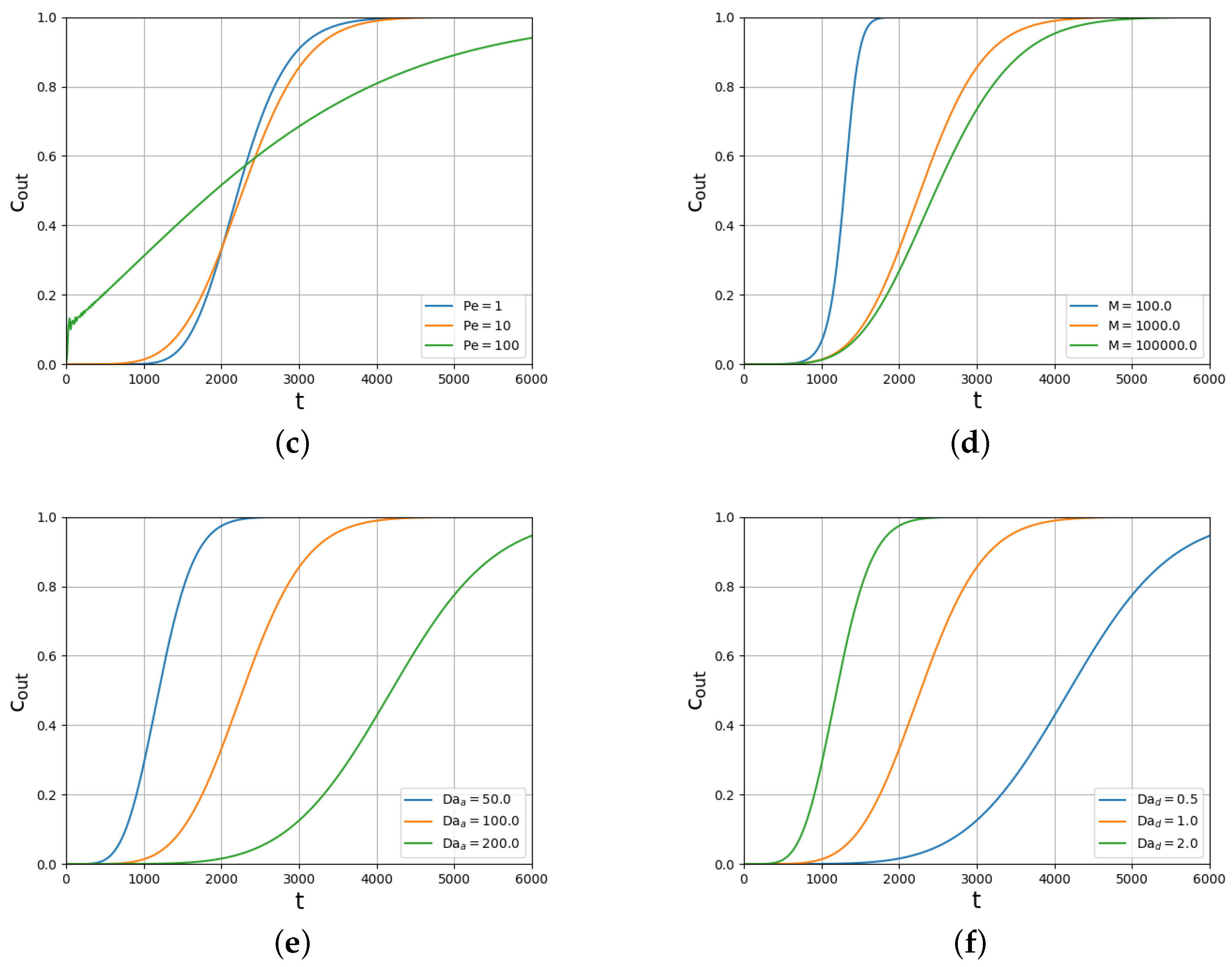
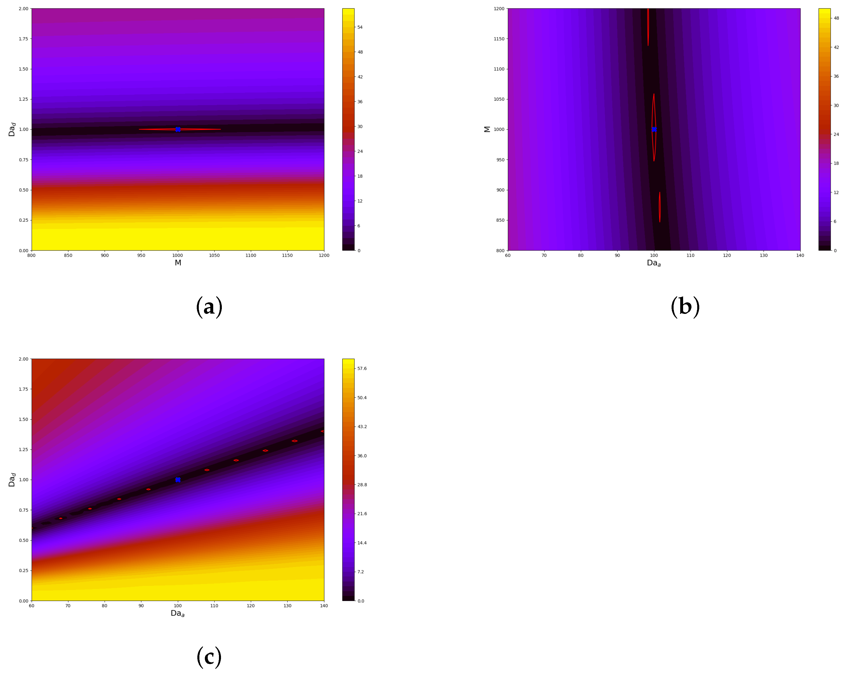
3.2. Geometry and Sensitivity Analysis

The computational domain is a rectangle with a dimensionless height of $x_2=1$ and dimensionless length of $x_1=17.5$, in which 10 half cylinders are embedded. The distance between the centers of the cylinders in the $x_1$ direction is 1.5 dimensionless units, and the radius of the cylinders is 0.4 dimensionless units.

The computational domain ${\mathsf{\Omega }}_f$ is triangulated using the grid generator Gmsh [42]. The script for preparing the geometry is written in Python. A demonstration of the computational grid is shown in Figure 2.

For the FEM approximation of the velocity, the pressure, and the respective test functions, the following finite dimensional subspaces are selected: ${\mathit{V}}_h\subset \mathit{V}$, ${\widehat{\mathit{V}}}_h\subset \widehat{\mathit{V}}$ and $Q_h\subset Q$. Taylor–Hood $P_2-P_1$ elements [43] are used here. These are continuous $P_2$ Lagrange elements for the velocity components and continuous $P_1$ Lagrange elements for the pressure field. The computations are carried out using the computing platform for partial differential equations FEniCS (website fenicsproject.org) [44,45].

As mentioned above, slow flows are mainly of interest for the current study. The convergence of the solution with respect to the refinement of the grid is illustrated in Figure 3a. The convergence of the solution with respect to the time step is illustrated in Figure 3b. We have used three computational grids: a basic grid with 18,743 nodes and 35,958 triangles, a coarse grid with 4760 nodes and 8754 triangles and a fine grid with 72,745 nodes and 142,460 triangles. From the results, it can be concluded that the coarse grid provides good enough accuracy for the numerical solution. Taking into account that we will solve a multitude of direct problems, it was decided to conduct research on a coarse grid.

A sensitivity study is carried out in order to identify how the change of different parameters leads to changes in the breakthrough curves:

• $\mathrm{Pe}=[1,10,100]$;
• ${\mathrm{Da}}_a=[50,100,200]$;
• ${\mathrm{Da}}_d=[0.5,1,2]$;
• $\mathrm{M}=[100,1000,100,000]$.

Such sensitivity studies are often tge first stage for optimization or parameter identification procedures. The dependence of the average outlet concentration from the Peclet number is shown in Figure 3c.

The rate of adsorption is characterized by ${\mathrm{Da}}_a$. The influence of this parameter on the outlet concentration is illustrated in Figure 3e. Increasing ${\mathrm{Da}}_a$, as expected, leads to more intensive adsorption and a larger amount of the deposited substance. The influence of the parameter ${\mathrm{Da}}_d$ on the outflow concentration is illustrated in Figure 3f.

The Henry isotherm usually describes the initial stages of the adsorption well. In cases when only a limited mass can be adsorbed at a surface, the Langmuir isotherm should be used to reflect the decay of the adsorption rate close to the saturation. In this case, an additional parameter appears, namely $\mathrm{M}$. The influence of $\mathrm{M}$ on the average output concentration is shown in Figure 3d.

The results are illustrated in Figure 3c–f. The curve in these figures is a breakthrough curve, which describes how much solute has crossed the outflow boundary, and it is given by

$$c_{out}\left(t\right)=\frac{{\int }_{{\mathsf{\Gamma }}_{out}}c(\mathit{x},t)d\mathit{x}}{{\int }_{{\mathsf{\Gamma }}_{out}}d\mathit{x}}.$$

(20)

4. Bee Colony Algorithms

There are many different modifications to this algorithm. The bees algorithm was first described by Pham and Ghanbarzadeh et al. in 2005 [26,27]. It mimics the food foraging behavior of honey bee colonies. More about the effectiveness and specific abilities of this algorithm can be found in [28,29,30]. The artificial bee colony (ABC) algorithm was introduced by Karaboga in 2005 [33]. This algorithm is a swarm-based metaheuristic algorithm. For details on the performance and convergence of the algorithm, we refer, e.g., to [34,35]. These two algorithms are very similar in terms of local and global search processes. However, there is a difference between both algorithms during the neighborhood search process. The ABC has a probabilistic approach during the neighborhood stage; however, the bees algorithm does not use any probability approach, but instead uses fitness evaluation to drive the search. Advantages of this family of algorithms are their applicability to non-convex functionals, the possibility to generalize to any dimension, and the high parallelism.

4.1. A Modified Bee Colony Algorithm

In this work, a modification of the bees algorithm will be presented, with the aim of adapting it to parameter identification problems related to reaction-dominated pore-scale transport, thus requiring mimization of the functional (21). A non-convex optimization problem has to be solved in this case, and the functional has the shape of a narrow valley with steep banks. Further on, in our case, we do not look for a point of global extremum; rather, we look for a subset in the parameter space for which the functional is below the prescribed threshold.

Let us describe the idea of the MBC algorithm used here. There are scout bees $sb$ that conduct random searches. After exploring the area, judging by the amount of nectar found, the area is divided into several local areas. To divide the search area into local areas, the Euclidean distance is used. This is done with the aim of effectively locating local areas so that at the initial stage they do not intersect with each other. The areas are ranged by the amount of nectar found in each of them. The first n areas are called the best locations where more agent bees $abb$ per area go; the rest of the m areas are called perspective locations, and fewer agent bees $abp$ go to each of them. Local areas are centered on the points which were identified by the scout bees, and the areas can be rectangular or circular in shape. The sizes of local areas should be chosen by an educated guess depending on the ranges of the parameters. All bees working in their locations can search around their area to increase the amount of nectar. If the bees cannot improve the result within a certain time $\tau$, they narrow their search area $\xi$ times. The algorithm stops if the distance between the found extrema in local areas reaches a given distance ${\epsilon }_1$ or the size of the local area becomes smaller than ${\epsilon }_2$. The threshold ${\epsilon }_2$ is problem dependent.

In general, our implementation of the algorithm requires the following control parameters, namely:

-

The number of best locations, n;

-

The number of perspective locations, m;

-

The local area side lengths $\mathbf{d}=\{d_1,d_2,\dots ,d_i\}$, where i here stands for the dimension of the problem;

-

The Euclidean distance value between two points in the parameter space, $\delta$;

-

The number of scout bees, $sb$;

-

The number of agent bees at the best locations, $abb$;

-

The number of agent bees on perspective locations, $abp$;

-

The maximum number of iterations allowed for one location $\tau$ before shrinking;

-

The stopping criteria ${\epsilon }_1$ and ${\epsilon }_2$ to control the distance between the best locations in one local area for two consecutive iterations and to control the size of the local area, respectively.

Uniform distribution is used to place the scout bees in the full domain at the beginning, as well as to place bees within each local area at each iteration over the area. The shapes of the local subdomains are rectangular. The algorithm is listed in Algorithm 1.

Let us shortly discuss the peculiarities of the MBC algorithm used here:

-

This algorithm demonstrates competent division into local areas through the Euclidean distance;

-

The shrinkage of the area occurs after $\tau$ unsuccessful attempts, not after every failure, thus reducing the chance to miss local minima;

-

The shrinkage of the area is aggressive in order to achieve faster convergence and higher accuracy (it is adapted for the class of problems considered here);

-

When a local extremum is found, it is stored, and the bees from the local area disappear; at the same time, the search in the other local areas continues;

-

The stopping criteria is checked for each location individually.

Let us now provide some more explanations concerning each item above.

The BA family is conceptually developed to search only for the global extremum; therefore, after each iteration, the values of the functional are sorted globally, and the few most perspective points are selected to continue the search. In our modification, the sorting and the selection are done locally for each local active area, thus enabling the local extrema to be found.

In the original algorithm, the area is shrunk once no improvement of the results is observed after the current iteration. Instead, in our modification, $\tau$ iterations are allowed before the area is shrunk. This allows the density of the bees exploring the area to be increased. Such a variant has advantages for functionals like the one considered here. One can start with a small number of bees per local area, and thus, in a cheap way, go down close to the bottom of the valley. Close to the bottom of the valley is relatively flat, so the density of the bees has to be increased. This is done either by repeated search in the same area, or by shrinking.

Algorithm 1: A modified Bee Colony algorithm pseudo-code.

Aggressive shrinking of the local area is explored in our case, unlike the most known bee-type algorithms, having in mind the shape of the considered functional. Each dimension of the respective local area is halved during shrinking. This allows for the computational costs to be reduced and the accuracy to be improved.

The SBA introduced the concept of the local area abandonment procedure. When a site is abandoned, the bee becomes a scout and the search process begins in a new place. In our modification, there is no concept of local area abandonment, since the local extrema are sought in addition to the global extremum. In our approach, the stopping criteria is checked for each local area and not globally.

4.2. Benchmark Testing

The MBC algorithm presented here was implemented in Python. To evaluate its performance, and to compare it to the performance of the widely used ABC algorithm [33], runs were carried out to find global and local minimums of well-known test functions. Despite the fact that all the functions below are generalized for a multidimensional case, and the algorithms can easily be implemented in multidimensional cases, in this work, only a two-dimensional case is explored to allow for easy visualization and to reduce the computational time. The following functions are considered:

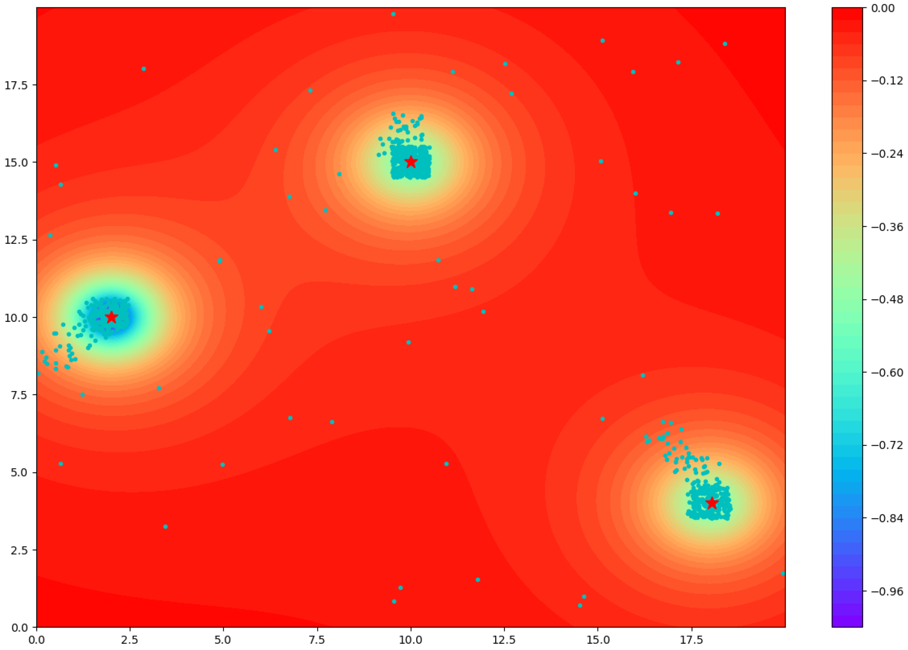
• Shekel function. This is a multidimensional, multimodal, continuous, deterministic function commonly used as a test function for testing optimization techniques [46];
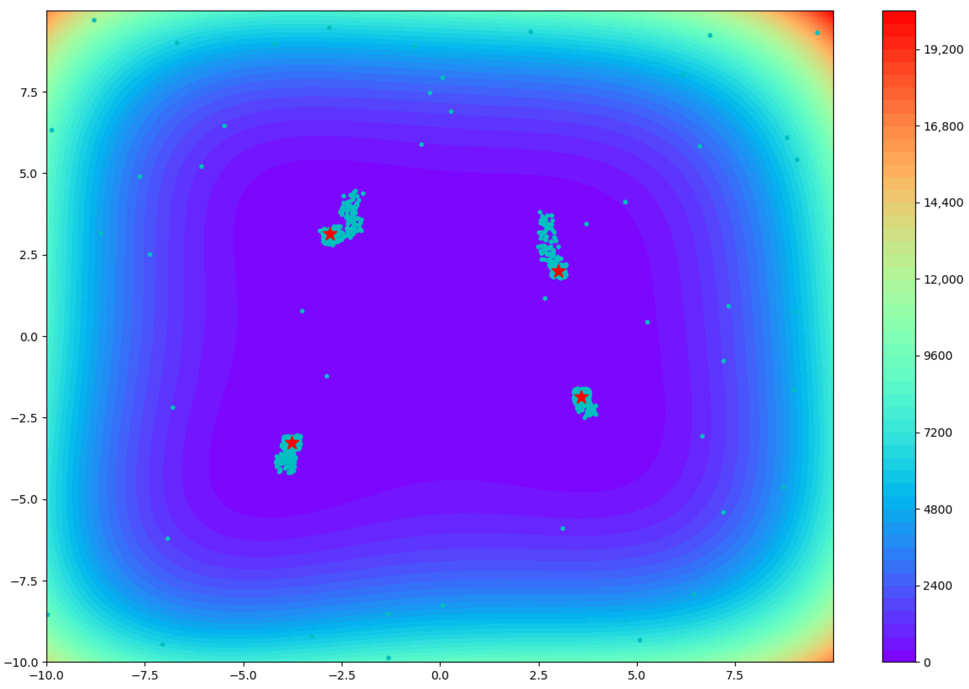
• Rosenbrock function. This is a non-convex function, introduced by Howard H. Rosenbrock in 1960 [47], which is used as a performance test problem for optimization algorithms. The global minimum is inside a long, narrow, parabolic-shaped flat valley. To find the valley is trivial. To converge to the global minimum, however, is difficult;
• Himmelblau function. This is a multi-modal function used to test the performance of optimization algorithms. The locations of all the minima can be found analytically. However, because they are roots of cubic polynomials, when written in terms of radicals, the expressions are somewhat complicated. The function is named after David Mautner Himmelblau, who introduced it [48];
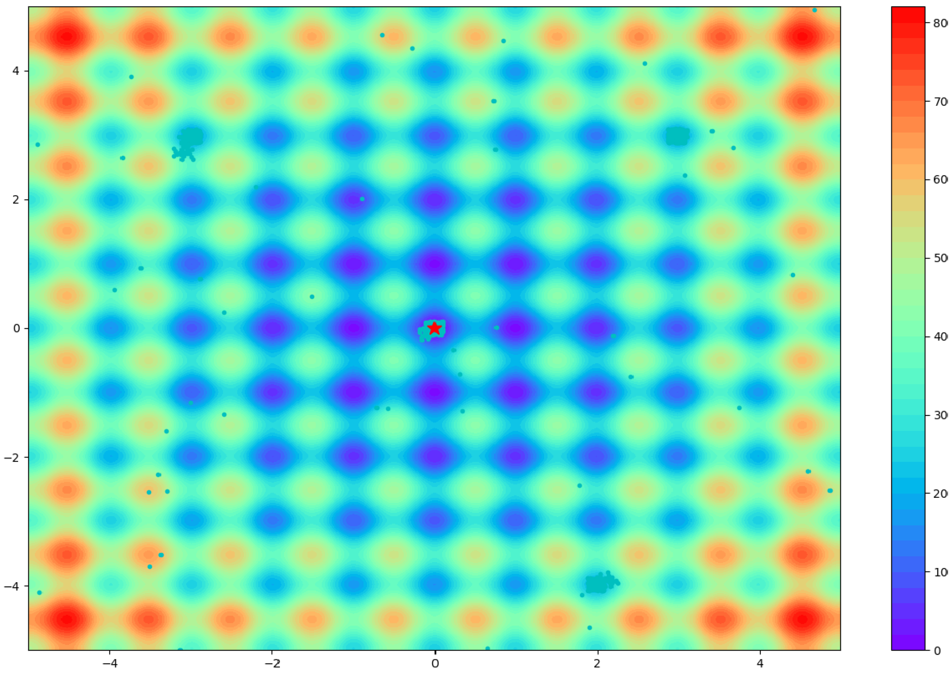
• Rastrigin function. This is a non-convex, non-linear multimodal function. It was first proposed by Rastrigin [49] as a 2-dimensional function and has been generalized by Rudolph [50]. The generalized version was popularized by Hoffmeister and Bäck [51] and Mühlenbein et al. [52]. Finding the minimum of this function is a fairly difficult problem due to its large search space and its large number of local minima.

The definition for each function can be seen in

Table 1. Benchmark definitions.

Function	Formulae	Range
Shekel	$F(x,y)=-\frac{1}{1+{(x-2)}^2+{(y-10)}^2}-\frac{1}{2+{(x-10)}^2+{(y-15)}^2}-\frac{1}{2+{(x-18)}^2+{(y-4)}^2}$	$[0,20]$
Rosenbrock	$F(x,y)=100{(y-x^2)}^2+{(1-x)}^2$	$[-5,5]$
Himmelblau	$F(x,y)={(x^2+y-11)}^2+{(x+y^2-7)}^2$	$[-10,10]$
Rastrigin	$F(x,y)=20+x^2+y^2-10(cos\left(2\pi x\right)+cos\left(2\pi y\right))$	$[-5,5]$

. The work of the MBC algorithm is illustrated in Figure 4, Figure 5, Figure 6 and Figure 7. The light blue spots represent processed points, while red stars indicate the extremum found in each location. These pictures are shown for the purpose of demonstrating the movement of the bees. The functions of Shekel and Himmelblau are quite simple in terms of finding extrema, so the number of the best locations and perspective locations in total were chosen the same as the number of the extrema. Since the functions of Rosenbrock and Rastrigin are rather complex functions, despite the fact that they have only one global minimum, we allowed the algorithm to work out more locations to increase the probability of success. Additionally, it is extremely important for us to control the number of function evaluations (NFE). The exact minima and the minima computed by MBC for the four benchmark functions are summarized in

Table 2. A modified bee colony algorithm.

Function	Minimum	Program Output	Iterations	NFE
Shekel	F(2,10) = −1.014 F(10,15) = −0.517 F(18,4) = −0.509	F(2.012, 10.005) = −1.014 F(9.991, 14.998) = −0.516 F(18.003, 4.008) = −0.509	93	1260
Rosenbrock	F(1,1) = 0	F(1.004, 1.009) = 9.134 × 10${}^{-5}$	138	1630
Himmelblau	F(3.584, −1.848) = 0 F(−2.805, 3.131) = 0 F(−3.779, −3.283) = 0 F(3, 2) = 0	F(3.579, −1.856) = 0.003 F(−2.804, 3.131) = 1.356 × 10${}^{-5}$ F(−3.777, −3.271) = 0.005 F(3.005, 2) = 0.001	113	1650
Rastrigin	F(0,0) = 0	F(−0.002, −0.005) = 0.005	96	1470

together with the number of iterations and NFE. As one can see, the algorithm works very well on all benchmarks.

For comparison, SBA and the more popular ABC algorithm were used to find the minima of the same benchmark functions. The results obtained with the SBA and ABC algorithms can be found in

Table 3. The standard bees algorithm.

Function	Minimum	Program Output	Iterations	NFE
Shekel	F(2,10) = −1.014 F(10,15) = −0.517 F(18,4) = −0.509	F(1.99, 10.014) = −1.014	24	4704
Rosenbrock	F(1,1) = 0	F(0.979, 0.962) = 9.474 × 10${}^{-4}$	53	8010
Himmelblau	F(3.584, −1.848) = 0 F(−2.805, 3.131) = 0 F(−3.779, −3.283) = 0 F(3, 2) = 0	F(−2.805, 3.132) = 5.681 × 10${}^{-5}$	38	2964
Rastrigin	F(0,0) = 0	F(9.251$\times {10}^{-6}$, 7.722 × 10${}^{-4}$) = 1.183 × 10${}^{-4}$	183	14,274

and

Table 4. Artificial bee colony algorithm.

Function	Minimum	Program Output	Iterations	NFE
Shekel	F(2,10) = −1.014 F(10,15) = −0.517 F(18,4) = −0.509	F(2.004, 10.018) = −1.014	215	4343
Rosenbrock	F(1,1) = 0	F(0.97, 0.94) = 9.039 × 10${}^{-4}$	1106	22,411
Himmelblau	F(3.584, −1.848) = 0 F(−2.805, 3.131) = 0 F(−3.779, −3.283) = 0 F(3, 2) = 0	F(−2.803, 3.132) = 1.43 × 10${}^{-4}$	83	853
Rastrigin	F(0,0) = 0	F(−1.925 × 10${}^{-5}$, −4.321 × 10${}^{-4}$) = 3.712 × 10${}^{-5}$	161	1645

, respectively. In the case of convex functionals, the SBA algorithm works well, but problems arise for non-convex Rosenbrock and multimodal Rastrigin functions, where the algorithm converges very slowly. The results in Table 3 and Table 4 show that the SBA and ABC algorithms only find the global minimum. Although these algorithms are based on the same idea, conceptually and algorithmically, they are different.

Results from comparative statistical analysis between SBA, ABC and MBC are summarized in

Table 5. Statistical comparison between SBA, ABC and MBC.

	Standard Bees Algorithm		Artificial Bee Colony		Modified Bee Colony
Function	Success	NFE (Mean)	Success	NFE (Mean)	Success	NFE (Mean)
Shekel	100%	3646	100%	2582	100%	502
Rosenbrock	100%	3850	100%	40,496	100%	2351
Himmelblau	100%	4352	100%	1431	100%	2007
Rastrigin	100%	11,220	100%	2806	48%	4274

. The average value of the NFEs was the main criterion in the comparison. We performed 100 independent runs for all algorithms. The parameter values used in relation to SBA, ABC and MBC are listed in

Table 6. SBA parameters.

Function	$\mathit{ne}$	$\mathit{nb}$	$\mathit{ngh}$	$\mathit{\delta }$	$\mathit{ns}$	$\mathit{nre}$	$\mathit{nrb}$	$\mathit{stlim}$
Shekel	1	2	{1, 1}	5	50	20	10	5
Rosenbrock	1	2	{0.4, 0.4}	4	50	20	10	5
Himmelblau	1	2	{0.4, 0.4}	4	50	20	10	5
Rastrigin	1	2	{0.2, 0.2}	1	50	20	10	5

,

Table 7. ABC algorithm parameters.

Function	SN	D	Limit
Shekel	10	2	20
Rosenbrock	10	2	20
Himmelblau	10	2	20
Rastrigin	10	2	20

and

Table 8. MBC algorithm parameters.

Function	n	m	d	$\mathit{\delta }$	$\mathit{sb}$	$\mathit{abb}$	$\mathit{abp}$	$\mathit{\tau }$	${\mathit{\epsilon }}_1$	${\mathit{\epsilon }}_2$
Shekel	1	2	{1, 1}	5	150	20	10	5	${10}^{-5}$	${10}^{-3}$
Rosenbrock	1	2	{0.4, 0.4}	4	150	20	10	5	${10}^{-8}$	${10}^{-3}$
Himmelblau	4	0	{0.4, 0.4}	4	250	20	10	5	${10}^{-5}$	${10}^{-4}$
Rastrigin	1	0	{1, 1}	1	500	20	10	5	${10}^{-8}$	${10}^{-8}$

, respectively. The notations for the parameters used here are according to [31,53]. It is easy to see that the SBA does not perform well in the Rastrigin function because it has many local extrema, which is why it converges for a very long time. The ABC works fine in the Rastrigin function, but instead shows weak results in the Rosenbrock function. This is because the Rosebrock function is unimodal, and in our experiment, it has only two dimensions. Conceptually, the ABC should perform better at higher dimensions [33]. Our modification in general works very well, except for the Rastrigin function: the global extremum was reached only 48 times out of 100 launches. This happens because in our modification there is no concept of “global search” as in SBA; thus, the outcome of the algorithm is highly dependent on the initial distribution of scout bees. We can come to the conclusion that our MBC algorithm does not work well in conditions when there are many local extrema. Additionally, it is worth paying attention to the Himmelblau function. Our algorithm has more NFE than ABC. This is explained by the fact that all 4 extrema of the Himmelblau function are global and equal to 0. The ABC algorithm needs to find only one of them, while our MBC is made to search for all extrema.

5. Parameter Identification

Consider an inverse problem for determining unknown parameters in a Langmuir isotherm (13) (so-called parameter identification problem). The functional of the squared difference between computed and “measured” breakthrough curves, given by

$$J({\mathrm{Da}}_a,{\mathrm{Da}}_d,\mathrm{M})={\int }_0^T{(c_{out}\left(t\right)-\widehat{c\left(t\right)})}^{2}dt,$$

(21)

is to be minimized. Here, $\widehat{c\left(t\right)}$ is a breakthrough curve from “measurements”. In fact, this curve is produced by solving the forward problem using a selected set of parameters, to be called below the “exact parameters”. $\mathrm{Pe}=10,{\mathrm{Da}}_a=100,{\mathrm{Da}}_d=1,$ and $\mathrm{M}=1000$ (see Langmuir isotherm Equation (13)) are selected as exact values in this study. They are used to produce the “measurement breakthrough curve”. These parameters correspond to the reaction-dominated case.

Taking into account the convergence studies presented here with respect to the space and time steps, it was decided to use a finite element grid with 4760 nodes in the computational domain, along with time step $\tau =30.$

The functional (21) is plotted in Figure 8. For better visibility, three figures are shown. On each one of them, one of the three parameters ${\mathrm{Da}}_a,{\mathrm{Da}}_d,\mathrm{M}$ is fixed, and the functional is plotted against the other two. It can be seen that it is a non-convex functional, and the low values of the functional are allocated in a narrow valley with steep banks. One of the banks of the valley is concave, while the second is convex, thus making the identification of the parameters a challenging task.

Recall that we are interested in solving a specific class of parameter identification problems. The main goal is not to identify exactly the parameter set giving the minimum of the functional. The main goal is to identify at least several parameter sets for which the functional is smaller than a prescribed threshold. Such a class of parameter identification problems is of interest for some industries. Furthermore, depending on the particular industry, a reasonable threshold could be 1%, but also could be 20%.

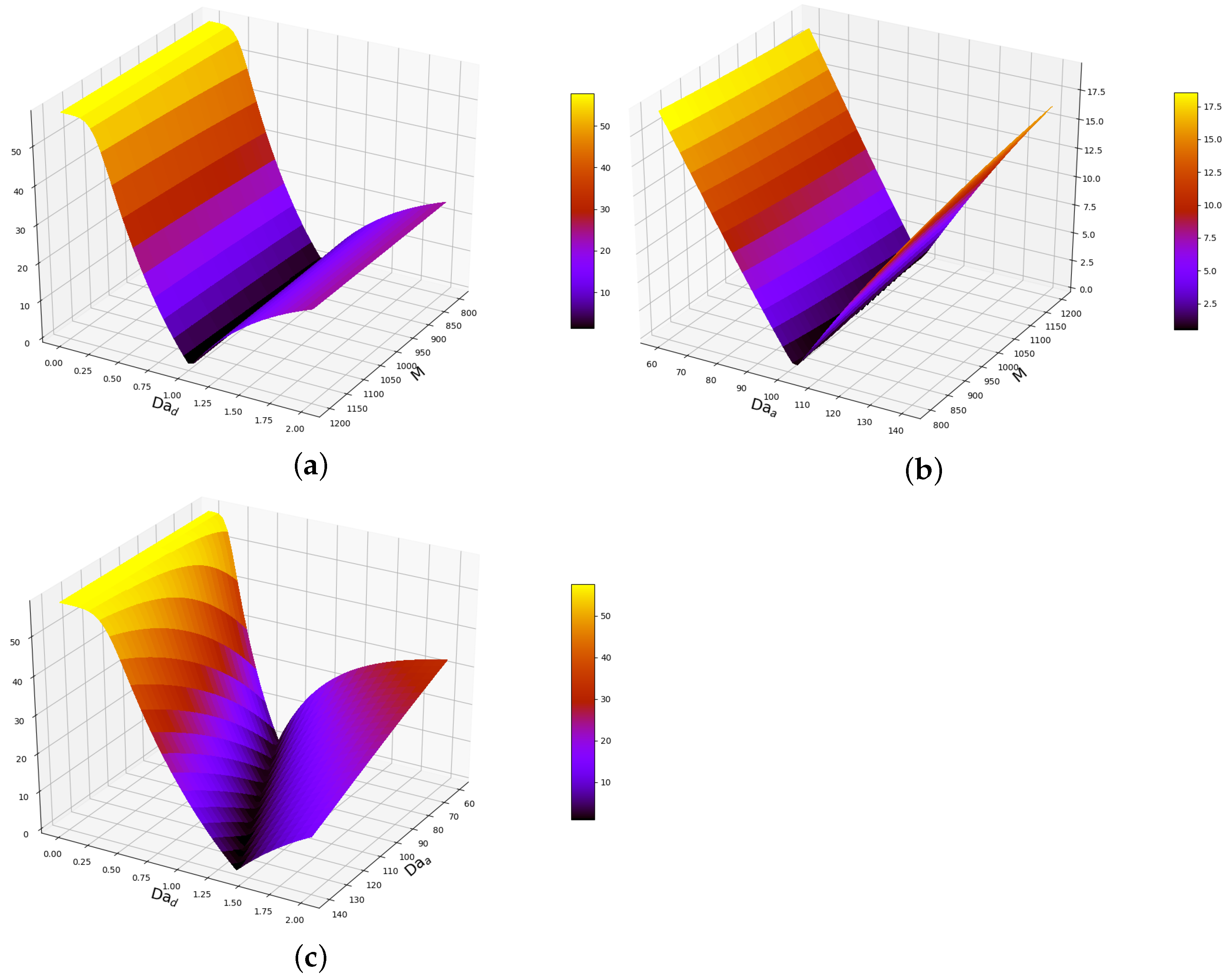
5.1. Reaction-Dominated Case, Deterministic Approach

The most simple approach to parameter identification is to consider a uniform grid in a proper subdomain of the parameter space, to compute the direct problem and the functional for each point of this grid, and to monitor the functional to find the minimum. Obviously this is a very inefficient way to identify the parameters because it requires a lot of solves for the direct problem; however, it is a reliable way to obtain a reference solution. This approach is presented here for comparison purposes. The parameters will be sought in the subdomain $60\le {\mathrm{Da}}_a\le 140$, $0\le {\mathrm{Da}}_d\le 2$, $800\le \mathrm{M}\le 1200$. A uniform grid $50\times 50\times 50$ is introduced in this subdomain. The forward problem is solved for each point from the grid, and the functional (21) is evaluated.

The computed results are shown in Figure 9. The blue star there denotes the exact parameters, while the red contour is an admissible set, which is defined as follows:

$$J({\mathrm{Da}}_{\mathrm{a}},{\mathrm{Da}}_{\mathrm{d}},\mathrm{M})\le 0.0246$$

(22)

The red contours surround admissible set of parameters, such that for all parameters from the admissible set, the functional is smaller than the prescribed threshold. It is easy to see that the admissible set captures the narrow valley with steep borders well, within which the smallest values of the functional are observed.

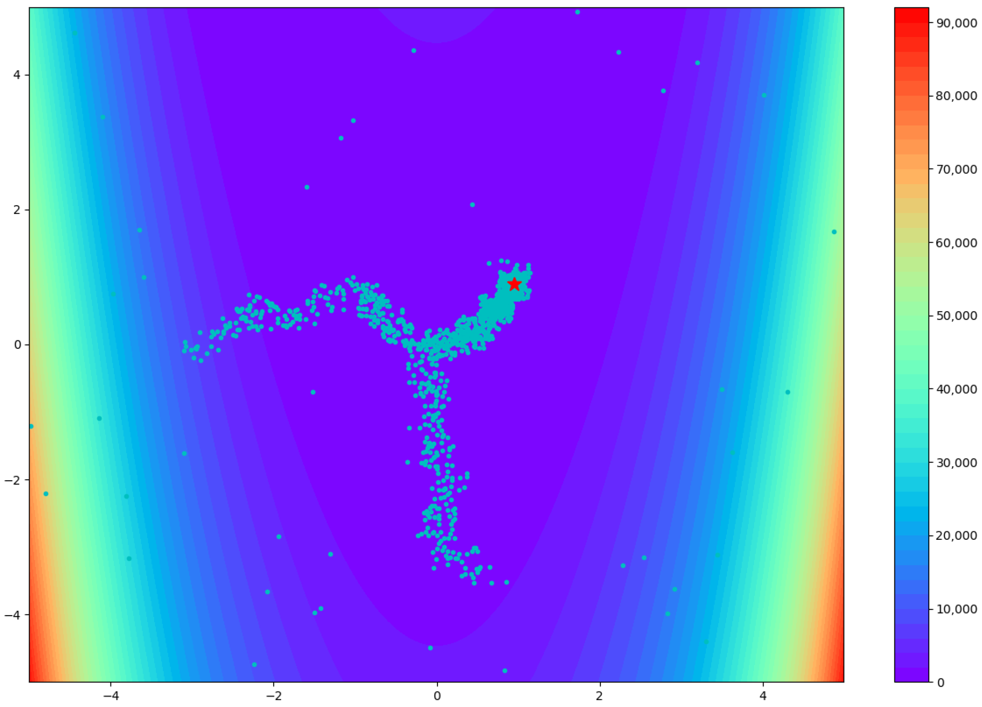
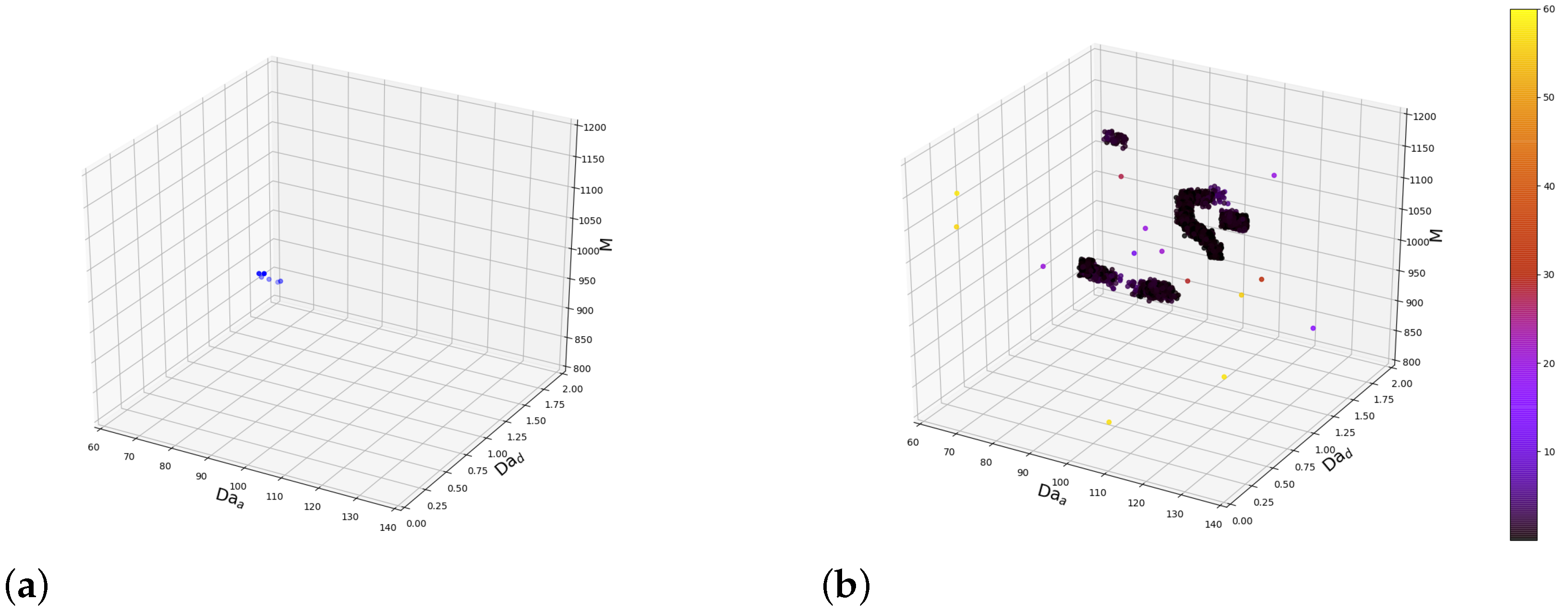
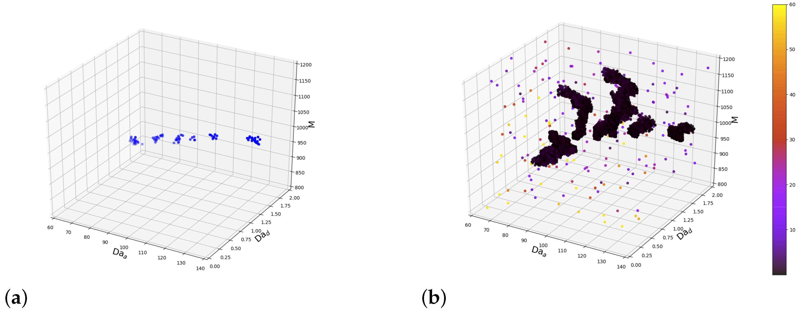
5.2. Reaction-Dominated Case, Modified Bee Colony Algorithm

The convergence of MBC, similar to the convergence of any BC algorithm, depends on the parameters of the algorithm. To illustrate this dependence, and at the same time to show that the algorithm converges for different sets of parameters, MBC is run with two sets of parameters here. Some parameters are the same for the both runs; these are: $n=2$, $d_x=6$, $d_y=0.06$, $d_z=20$, $\delta =1$, $abb=50$, $\tau =5,{\epsilon }_1={10}^{-8}$, ${\epsilon }_2=1$. The parameters which differ in the two runs are

I:

$m=3$, $sb=20$, $abb=50$, $abp=20$;

II:

$m=5$, $sb=200$, $abb=50$, $abp=40$.

The subdomain in which the reaction parameters are sought is selected to be the same as in the deterministic case above. Namely, X axis — parameter ${\mathrm{Da}}_a\in [60,140]$, Y axis — parameter ${\mathrm{Da}}_d\in [0,2]$, Z axis — parameter $\mathrm{M}\in [800,1200]$.

The five best identified points and the functional values there, together with the number of the iterations and the number of the direct solves, are summarized in

Table 9. Results for the reaction-dominated case.

Parameter Set I
Program output	Error (%)	Iterations	NFE
J(84.554, 0.845, 995.593) = 0.002	0.016	94	2230
J(112.266, 1.126, 1029.347) = 0.031	0.056
J(100.455, 1.001, 964.319) = 0.0477	0.08
J(116.173, 1.17, 1078.88) = 0.085	0.15
J(91.394, 0.928, 1200.789) = 0.213	0.374
Parameter Set II
Program output	Error (%)	Iterations	NFE
J(92.794, 0.928, 997.607) = 1.29$\times {10}^{-3}$	0.002	281	12,300
J(83.358, 0.833, 994.812) = 3.01$\times {10}^{-3}$	0.003
J(101.655, 1.017, 1000.054) = 4.2$\times {10}^{-3}$	0.007
J(136.404, 1.367, 1011.473) = 5.7$\times {10}^{-3}$	0.01
J(117.636, 1.178, 1014.271) = 0.011	0.02

. It is useful to also compare the relative error in computing the functional (the functional itself gives absolute error). The relative error is calculated as follows:

$${\mathcal{E}}_{rel}=\frac{\parallel c_{out}-\widehat{c_{out}}{\parallel }_2}{\parallel \widehat{c_{out}}{\parallel }_2}=\frac{\sqrt{{\sum }_{i=0}^{Nt}{(c_i-\widehat{c_i})}^2}}{\sqrt{{\sum }_{i=0}^{Nt}{\widehat{c_i}}^2}},$$

(23)

where $Nt$ is the number of the time intervals and $\widehat{c_{out}}$ is the selected exact solution (imitating data from experiments). The relative error is listed in the third column in Table 9.

It can be seen that for both MBC parameters sets, the Langmuir’s isotherm parameters which give very low values of the functional are identified. The second set of MBC parameters gives better results at the cost of more expensive computations. The computed relative error is less than 1% for the 5 selected points from the first run of MBC, and less than 0.02% for the second run, respectively.

Another important observation is that MBC is well adapted to the main goals of the paper, namely identifying not just the exact reaction parameters, but identifying the reaction parameter sets for which the residual takes small values.

A 3D visualization of the results is shown in Figure 10 and Figure 11. Figure 10b and Figure 11b illustrate the points from the parameter subdomain which are explored by MBC, while Figure 10a and Figure 11a show only those points for which the functional is smaller than the selected threshold.

Note that in many industrial problems, much higher error is tolerated. If the stopping criteria ${\epsilon }_1$ is increased from $1e-8$ to $1e-3$, and the following parameter set is used for MBC: $n=1$, $m=2$, $d_x=6$, $d_y=0.06$, $d_z=20$, $\delta =1$, $sb=20$, $abb=20$, $abp=5$, $\tau =3,{\epsilon }_1={10}^{-3}$, ${\epsilon }_2=1$, the following results are obtained; see

Table 10. Results for increased stopping criteria.

Program Output	Error (%)	Iterations	NFE
J(126.11, 1.287, 1151.449) = 0.362	0.626	16	205
J(104.861, 1.038, 991.051) = 0.405	0.7
J(117.213, 1.146, 927.115) = 0.654	1.133

.

It is remarkable that not only is a reasonable admissible set of parameters identified, but the global minimum is also computed accurately. Namely, by comparing the identified global minimum (126.11, 1.287, 1151.449) with the exact parameters (100, 1, 1000), the relative error of 0.626% is obtained.

6. Summary

The proposed modification of the SBA is capable of finding not only global extrema, but also local extrema. The algorithm showed good results on the Shekel, Rosenbrock, Himmelblau and Rastrigin benchmark functions. A comparative statistical analysis was performed with the usual SBA and the more popular ABC on 100 independent runs for each of the functions. Based on the results obtained, it can be concluded that the proposed MBC algorithm is able to quickly and accurately find all the extrema in the case of a moderate number of extrema. More important, it is demonstrated that the MBC can be used for parameter identification for an important class of problems. Admissible sets for the unknown parameters in Langmuir isotherms are identified in the case of reaction-dominated pore-scale reactive flow. The parameter identification problem for this regime is related to the minimization of a non-convex functional, characterized by a narrow valley with steep banks, which is relatively flat near the minimum.

References

1. Bear, J. Dynamics of Fluids in Porous Media; Courier Corporation: New York, NY, USA, 2013. [Google Scholar]
2. Helmig, R. Multiphase Flow and Transport Processes in the Subsurface: A Contribution to the Modeling of Hydrosystems; Springer: Berlin/Heidelberg, Germany, 1997. [Google Scholar]
3. Lavrent’ev, M.M.; Romanov, V.G.; Shishatskii, S.P. Ill-Posed Problems of Mathematical Physics and Analysis; American Mathematical Society: Providence, RI, USA, 1986. [Google Scholar]
4. Alifanov, O.M. Inverse Heat Transfer Problems; Springer: Berlin, Germany, 2011. [Google Scholar]
5. Isakov, V. Inverse Problems for Partial Differential Equations; Springer: New York, NY, USA, 2006; Volume 127. [Google Scholar]
6. Samarskii, A.A.; Vabishchevich, P.N. Numerical Methods for Solving Inverse Problems of Mathematical Physics; De Gruyter: Berlin, Germany, 2007. [Google Scholar]
7. Sun, N.Z. Inverse Problems in Groundwater Modeling; Springer Science & Business Media: Berlin/ Heidelberg, Germany, 2013; Volume 6. [Google Scholar]
8. Tarantola, A. Inverse Problem Theory and Methods for Model Parameter Estimation; SIAM: Philadelphia, PA, USA, 2005. [Google Scholar]
9. Aster, R.C.; Borchers, B.; Thurber, C.H. Parameter Estimation and Inverse Problems; Elsevier: Amsterdam, The Netherlands, 2013. [Google Scholar]
10. Tikhonov, A.N.; Arsenin, V.Y. Solutions of Ill-Posed Problems; V.H. Winston & Sons: New York, NY, USA, 1977. [Google Scholar]
11. Engl, H.W.; Groetsch, C.W. Inverse and Ill-Posed Problems; Elsevier: Amsterdam, The Netherlands, 2014; Volume 4. [Google Scholar]
12. Horst, R.; Pardalos, P.M. (Eds.) Handbook of Global Optimization; Springer: Berlin, Germany, 2013. [Google Scholar]
13. Nocedal, J.; Wright, S.J. Numerical Optimization, 2nd ed.; Springer Series in Operations Research and Financial Engineering; Springer: Berlin/Heidelberg, Germany, 2006. [Google Scholar]
14. Goldberg, D.E. Genetic Algorithms; Pearson Education: Karnataka, India, 2006. [Google Scholar]
15. Wei, Y.; Qiqiang, L. Survey on particle swarm optimization algorithm. Eng. Sci. 2004, 5, 87–94. [Google Scholar]
16. Sette, S.; Boullart, L. Genetic programming: Principles and applications. Eng. Appl. Artif. Intell. 2001, 14, 727–736. [Google Scholar] [CrossRef]
17. Storn, R.; Price, K. Differential evolution—A simple and efficient heuristic for global optimization over continuous spaces. J. Glob. Optim. 1997, 11, 341–359. [Google Scholar] [CrossRef]
18. Marques-Silva, J.P.; Sakallah, K.A. GRASP: A search algorithm for propositional satisfiability. IEEE Trans. Comput. 1999, 48, 506–521. [Google Scholar] [CrossRef] [Green Version]
19. Najari, S.; Gróf, G.; Saeidi, S.; Gallucci, F. Modeling and optimization of hydrogenation of CO2: Estimation of kinetic parameters via Artificial Bee Colony (ABC) and Differential Evolution (DE) algorithms. Int. J. Hydrogen Energy 2019, 44, 4630–4649. [Google Scholar] [CrossRef]
20. Yang, J.; Lu, L.; Ouyang, W.; Gou, Y.; Chen, Y.; Ma, H.; Guo, J.; Fang, F. Estimation of kinetic parameters of an anaerobic digestion model using particle swarm optimization. Biochem. Eng. J. 2017, 120, 25–32. [Google Scholar] [CrossRef]
21. Barbalho, T.J.; Santos, A.C.; Aloise, D.J. Metaheuristics for the Work-Troops Scheduling Problem. 2020. Available online: https://onlinelibrary.wiley.com/doi/abs/10.1111/itor.12925 (accessed on 10 November 2021).
22. Liu, Q.; Li, X.; Liu, H.; Guo, Z. Multi-objective metaheuristics for discrete optimization problems: A review of the state-of-the-art. Appl. Soft Comput. 2020, 93, 106382. [Google Scholar] [CrossRef]
23. Karimi-Mamaghan, M.; Mohammadi, M.; Meyer, P.; Karimi-Mamaghan, A.M.; Talbi, E.G. Machine learning at the service of meta-heuristics for solving combinatorial optimization problems: A state-of-the-art. Eur. J. Oper. Res. 2022, 296, 393–422. [Google Scholar] [CrossRef]
24. Franco-Sepúlveda, G.; Del Rio-Cuervo, J.C.; Pachón-Hernández, M.A. State of the art about metaheuristics and artificial neural networks applied to open pit mining. Resour. Policy 2019, 60, 125–133. [Google Scholar] [CrossRef]
25. Mehrabi, M.; Pradhan, B.; Moayedi, H.; Alamri, A. Optimizing an Adaptive Neuro-Fuzzy Inference System for Spatial Prediction of Landslide Susceptibility Using Four State-of-the-art Metaheuristic Techniques. Sensors 2020, 20, 1723. [Google Scholar] [CrossRef] [Green Version]
26. Pham, D.; Ghanbarzadeh, A.; Koc, E.; Otri, S.; Rahim, S.; Zaidi, M. The Bees Algorithm; Technical Note; Manufacturing Engineering Centre, Cardiff University: Cardiff, UK, 2005. [Google Scholar]
27. Pham, D.T.; Ghanbarzadeh, A.; Koç, E.; Otri, S.; Rahim, S.; Zaidi, M. The bees algorithm—A novel tool for complex optimisation problems. In Intelligent Production Machines and Systems; Elsevier: Amsterdam, The Netherlands, 2006; pp. 454–459. [Google Scholar]
28. Pham, D.T.; Castellani, M. The bees algorithm: Modelling foraging behaviour to solve continuous optimization problems. Proc. Inst. Mech. Eng. Part C J. Mech. Eng. Sci. 2009, 223, 2919–2938. [Google Scholar] [CrossRef]
29. Pham, D.T.; Castellani, M. Benchmarking and comparison of nature-inspired population-based continuous optimisation algorithms. Soft Comput. 2014, 18, 871–903. [Google Scholar] [CrossRef]
30. Pham, D.T.; Castellani, M. A comparative study of the Bees Algorithm as a tool for function optimisation. Cogent Eng. 2015, 2, 1091540. [Google Scholar] [CrossRef]
31. Baronti, L.; Castellani, M.; Pham, D.T. An analysis of the search mechanisms of the bees algorithm. Swarm Evol. Comput. 2020, 59, 100746. [Google Scholar] [CrossRef]
32. Hussein, W.A.; Sahran, S.; Abdullah, S.N.H.S. The variants of the Bees Algorithm (BA): A survey. Artif. Intell. Rev. 2017, 47, 67–121. [Google Scholar] [CrossRef]
33. Karaboga, D.; Akay, B. An Artificial Bee Colony (ABC) Algorithm on Training Artificial Neural Networks; Technical Report TR06; Erciyes University, Engineering Faculty, Computer Engineering Department: Kayseri, Turkey, 2005. [Google Scholar]
34. Karaboga, D.; Basturk, B. On the performance of artificial bee colony (ABC) algorithm. Appl. Soft Comput. 2008, 8, 687–697. [Google Scholar] [CrossRef]
35. Karaboga, D.; Akay, B. A comparative study of artificial bee colony algorithm. Appl. Math. Comput. 2009, 214, 108–132. [Google Scholar] [CrossRef]
36. Kralchevsky, P.A.; Danov, K.D.; Denkov, N.D. Handbook of Surface and Colloid Chemistry; Chapter Chemical Physics of Colloid Systems and Interfaces; Taylor & Francis Group, LLC: Abingdon, UK, 2009; pp. 197–377. [Google Scholar]
37. Grigoriev, V.V.; Iliev, O.; Vabishchevich, P.N. Computational identification of adsorption and desorption parameters for pore scale transport in periodic porous media. J. Comput. Appl. Math. 2019, 370, 112661. [Google Scholar] [CrossRef]
38. Grigoriev, V.V.; Vabishchevich, P.N. Bayesian Estimation of Adsorption and Desorption Parameters for Pore Scale Transport. Mathematics 2021, 9, 1974. [Google Scholar] [CrossRef]
39. Acheson, D.J. Elementary Fluid Dynamics; Clarendon Press: Oxford, UK, 2005. [Google Scholar]
40. Churbanov, A.G.; Iliev, O.; Strizhov, V.F.; Vabishchevich, P.N. Numerical simulation of oxidation processes in a cross-flow around tube bundles. Appl. Math. Model. 2018, 59, 251–271. [Google Scholar] [CrossRef] [Green Version]
41. Gresho, P.M.; Sani, R.L. Incompressible Flow and the Finite Element Method, Volume 2, Isothermal Laminar Flow; Wiley: New York, NY, USA, 2000. [Google Scholar]
42. Geuzaine, C.; Remacle, J.F. Gmsh: A three-dimensional finite element mesh generator with built-in pre- and post-processing facilities. Int. J. Numer. Methods Eng. 2009, 79, 1309–1331. [Google Scholar] [CrossRef]
43. Taylor, C.; Hood, P. A numerical solution of the Navier-Stokes equations using the finite element technique. Comput. Fluids 1973, 1, 73–100. [Google Scholar] [CrossRef]
44. Logg, A.; Mardal, K.A.; Wells, G.N. Automated Solution of Differential Equations by the Finite Element Method; Springer: Berlin/Heidelberg, Germany, 2012. [Google Scholar] [CrossRef]
45. Alnæs, M.S.; Blechta, J.; Hake, J.; Johansson, A.; Kehlet, B.; Logg, A.; Richardson, C.; Ring, J.; Rognes, M.E.; Wells, G.N. The FEniCS Project Version 1.5. Arch. Numer. Softw. 2015, 3, 9–23. [Google Scholar] [CrossRef]
46. Shekel, J. Test functions for multimodal search techniques. In Proceedings of the Fifth Annual Princeton Conf. on Information Science and Systems, Princeton, NJ, USA, 25–26 March 1971. [Google Scholar]
47. Rosenbrock, H. An automatic method for finding the greatest or least value of a function. Comput. J. 1960, 3, 175–184. [Google Scholar] [CrossRef] [Green Version]
48. Himmelblau, D.M. Applied Nonlinear Programming; McGraw-Hill: New York, NY, USA, 1972. [Google Scholar]
49. Rastrigin, L. Extremal Control Systems. Cybernetics Series; Theoretical Foundations of Engineering: Nauka, Russian, 1974; Volume 3. [Google Scholar]
50. Rudolph, G. Globale Optimierung Mit Parallelen Evolutionsstrategien. Ph.D. Thesis, Universit at Dortmund, Fachbereich Informatik, Dortmund, Germany, 1990. [Google Scholar]
51. Hoffmeister, F.; Bäck, T. Genetic algorithms and evolution strategies: Similarities and differences. In International Conference on Parallel Problem Solving from Nature; Springer: Berlin/Heidelberg, Germany, 1990; pp. 455–469. [Google Scholar]
52. Mühlenbein, H.; Schomisch, M.; Born, J. The parallel genetic algorithm as function optimizer. Parallel Comput. 1991, 17, 619–632. [Google Scholar] [CrossRef]
53. Song, X.; Zhao, M.; Yan, Q.; Xing, S. A high-efficiency adaptive artificial bee colony algorithm using two strategies for continuous optimization. Swarm Evol. Comput. 2019, 50, 100549. [Google Scholar] [CrossRef]
Figure 1. Sketch of the pore scale domain.
Algorithms 15 00015 g001
Figure 2. Computational grid.
Algorithms 15 00015 g002
Figure 3. Research on: (a) computational grids of different densities, (b) different time steps, (c) different Peclet numbers, (d) different maximum concentrations adsorbed on the surface, (e) different Damköler numbers for adsorption, (f) different Damköler numbers for desorption.
Algorithms 15 00015 g003aAlgorithms 15 00015 g003b
Figure 4. Rosenbrock function.
Algorithms 15 00015 g004
Figure 5. Shekel function.
Algorithms 15 00015 g005
Figure 6. Himmelblau function.
Algorithms 15 00015 g006
Figure 7. Rastrigin function.
Algorithms 15 00015 g007
Figure 8. 3D plots for fixed: (a) Da a , (b) Da d , (c) M .
Algorithms 15 00015 g008
Figure 9. Calculations for fixed: (a) Da a , (b) Da d , (c) M .
Algorithms 15 00015 g009
Figure 10. Results of the algorithm for parameter set I: (a) below threshold (22), (b) functional (21).
Algorithms 15 00015 g010
Figure 11. Results of the algorithm for parameter set II: (a) below threshold (22), (b) functional (21).
Algorithms 15 00015 g011