Article

Searching Monotone Arrays: A Survey

by
Márcia R. Cappelle
,
Les R. Foulds
and
Humberto J. Longo
*,†
Instituto de Informática, Universidade Federal de Goiás, Goiânia 74690-900, Brazil
*
Author to whom correspondence should be addressed.
These authors contributed equally to this work.
Algorithms 2022, 15(1), 10; https://doi.org/10.3390/a15010010
Submission received: 13 November 2021 / Revised: 13 December 2021 / Accepted: 22 December 2021 / Published: 26 December 2021
(This article belongs to the Special Issue Surveys in Algorithm Analysis and Complexity Theory)

Abstract

:
Given a monotone ordered multi-dimensional real array A and a real value k, an important question in computation is to establish if k is a member of A by sequentially searching A by comparing k with some of its entries. This search problem and its known results are surveyed, including the case when A has sizes not necessarily equal. Worst case search algorithms for various types of arrays of finite dimension and sizes are reported. Each algorithm has order strictly less than the product of the sizes of the array. Present challenges and open problems in the area are also presented.

1. Introduction

Searching is one of the most basic, frequent and important operations performed in tasks involving computation. A common challenge involves searching to decide whether or not a given real value (termed a key) is present in a given multi-dimensional array of real values. When the search must be performed sequentially and repeatedly by comparing the key with selected entries of the array, obviously it should be carried out as efficiently as possible by minimising the number of comparisons. This classic problem can be viewed as determining the correct dimensional threshold function from a finite class of such functions within the array, based on sequential queries that take the form of point samples. The complexity of such a search is completely dependent on how the array is organised.
Clearly, when there is no information available about array organisation, every entry must be examined. An array is termed monotone nondecreasing (nonincreasing) if its entries never decrease (increase) when moving away from the origin along any path parallel to an axis. Without loss of generality, from now on in the present article, the focus is on only monotone nondecreasing arrays. When the array is already sorted so that its entries are monotone nondecreasing, the search for a key can be conducted in a far more efficient manner compared to the unsorted case.
The problem addressed here is to search for a given real-valued key in a monotone nondecreasing multi-dimensional real array, that has sizes that are not necessarily equal. The challenge is to identify among all possible suitable search algorithms, one with the lowest complexity, i.e., requiring the minimum number of comparisons in the worst case. The main question being addressed until the end of Section 7 of the present article is to ask if the key is present in the array. Thus, if an instance of the key is found, there is no necessity to identify further possible instances of the key and the search procedure is terminated. The search for all possible occurrences of the key is briefly discussed in Section 8.
This important search problem occurs in many computation-related fields, including computational biology, image processing, VLSI design, operations research and statistics [1,2,3,4]. The main contributions of this survey are:
  • an introduction to the problem of searching a (strictly) monotone real array;
  • a discussion of known results and the description of worst-case algorithms;
  • conclusions that can be drawn from the discussions and descriptions and
  • proposals for future work on the open problems that have been identified.
Currently, asymptotic notation to express the complexity of algorithms is commonly used. However, many of the algorithms described here were formally described and analysed at a time when this notation was not so common. The work of Linial and Saks [5], for example, although using asymptotic notation, proposed exact lower and upper bounds on the number of comparisons necessary to determine the occurrence, or not, of a given element in an ordered array. Since then, many other authors have followed the same practice. Thus, for consistency with many of these works and due to the importance of these bounds in understanding the efficiency of the various algorithms listed here, the analyses of many of them are presented as originally developed by the respective authors. However, sometimes, asymptotic notation is used as a complementary tool for describing the complexity of algorithms.
The remainder of this paper is organised as follows. Preliminary notation, terminology and basic concepts are provided in the next section. What has been reported in the open literature on searching arrays to establish if a given key is present is reported in Section 3, Section 4, Section 5 and Section 6. The search of vectors ( d = 1 ) is the object of Section 3. Seven different algorithms for this case were identified in the literature, from basic linear search algorithms of non-ordered vectors to binary search of ordered matrices. The other algorithms are Jump Search (Block Search), Interpolation Search, Exponential Search, Fibonacci Search and Ternary Search and its generalisation (k-nary Search). The search of matrices (when d = 2 ) is explored in Section 4. Three algorithms are described: Saddleback Search for the case of balanced matrices and Shen’s and Bird’s algorithms for unbalanced matrices. Two algorithms for searching cuboids ( d = 3 ), one for the balanced case (the L&S algorithm) and one for the unbalanced case (an extension of Shen’s and Bird’s methods), are described in Section 5. Section 6 contains a description of a search algorithm for hypercubes when d 4 (denoted as Cheng-4). Section 7 discusses in some detail aspects of the worst case performance of some of the revised algorithms.
Many of the algorithms mentioned above call a binary search algorithm as a subroutine. This algorithm, as well its history, asymptotic complexity and some of its variants, are discussed in detail in Section 3 and Section 7.1. While the main focus of this survey is on the problem of verifying the occurrence or not of a key in monotone arrays, the challenge of searching for all occurrences of the key is also briefly discussed in Section 8. The paper ends with a summary, some concluding remarks and suggestions for future work on problems that remain open, which are presented in Section 9.

2. Preliminaries

Consider a real d-dimensional array A = { a ( i 1 , i 2 , , i d ) i 1 = 1 , , n 1 ; i 2 = 1 , , n 2 ; ; i d = 1 , , n d } , that is monotone nondecreasing in the sense that a ( i 1 , i 2 , , i d ) a ( j 1 , j 2 , , j d ) if i 1 j 1 , i 2 j 2 , , i d j d , for given, independent, sizes n 1 , n 2 , , n d Z + , (i.e., the entries of A are nondecreasing along its dimensions). A can be thought of as equivalent to the product of the chains [ n 1 ] , [ n 2 ] , , [ n d ] of the partially ordered sets { 1 , , n 1 } , { 1 , , n 2 } , , { 1 , , n d } .
A d-dimensional array A can be also defined by the indexes of its lower corner and upper corner as A ( ( 1 , 1 , , 1 ) , , ( n 1 , n 2 , , n d ) ) . Similarly, a d-dimensional subarray of A is defined as A ( ( 1 , 2 , , d ) , , ( r 1 , r 2 , , r d ) ) , where 1 i r i n i , for all 1 i d .
The problem discussed here involves searching A in order to establish whether or not a given key x R is a member of A. It is assumed that the search must be carried out by sequentially comparing x with selected entries a ( i 1 , i 2 , , i d ) A . The purpose of such comparisons is to eliminate elements of A and search the remaining subarrays in an efficient manner. It is of interest to identify search algorithms that require the minimum number of comparisons in the worst case.
When comparing x and any entry a ( i 1 , i 2 , , i d ) , one of the three following results must be obtained:
x < a ( i 1 , i 2 , , i d ) ,
in which case the entries a ( j 1 , j 2 , , j d ) for j 1 i 1 , j 2 i 2 , , j d i d , can be discarded; or
x = a ( i 1 , i 2 , , i d ) ,
in which case x has been located and the search is terminated; or
x > a ( i 1 , i 2 , , i d ) ,
in which case the entries a ( j 1 , j 2 , , j d ) for j 1 i 1 , j 2 i 2 , , j d i d , can be discarded. It is clear that it is necessary to make two comparisons between x and any entry a ( i 1 , i 2 , , i d ) to cover the three possibilities (1)–(3).
Any entry that is discarded by the comparison process as (1) and (3) above (as it cannot possibly be x) is termed redundant. If, in carrying out the comparison process, an entry a ( i 1 , i 2 , , i d ) of A, causes A to be divided into at least two nondegenerate subarrays, then this entry is termed a pivot.
An array A is said to be α -balanced if n i α · n i + 1 , 1 i d 1 , for a given α R + , 1 α 6.4 . The use of the constant 6.4 is justified in the arguments given towards the end of Section 4.2. A 1-balanced array is termed balanced, where n 1 = n 2 = = n d = n ( 2 ) say, and is a hypercube. If n i > 6.4 · n i 1 , 2 i d , A is termed unbalanced. If the sizes of A are strictly unequal, A is a rectangular hypercuboid. From now on, all cuboids and hypercuboids to be searched will be assumed to be rectangular and the term rectangular will be dropped.
Suppose A is a d-dimensional array with sizes n 1 , , n d . Let M ( A ) be the the minimum number of comparisons (taken over all possible search algorithms) needed either to establish whether or not a given key x is in A. We denote M ( A ) by.
M ( A ) = τ ( n , d ) , if A is balanced and n 1 = = n d = n ; ϕ ( n 1 , , n d ) , otherwise .
When calculating the asymptotic time complexity of an algorithm, in general, the constant term in M ( A ) can be neglected. However, if an exact count of the number of comparisons is required, the constant term should be included. This has been done when establishing the time complexity of many of the algorithms described in this survey.
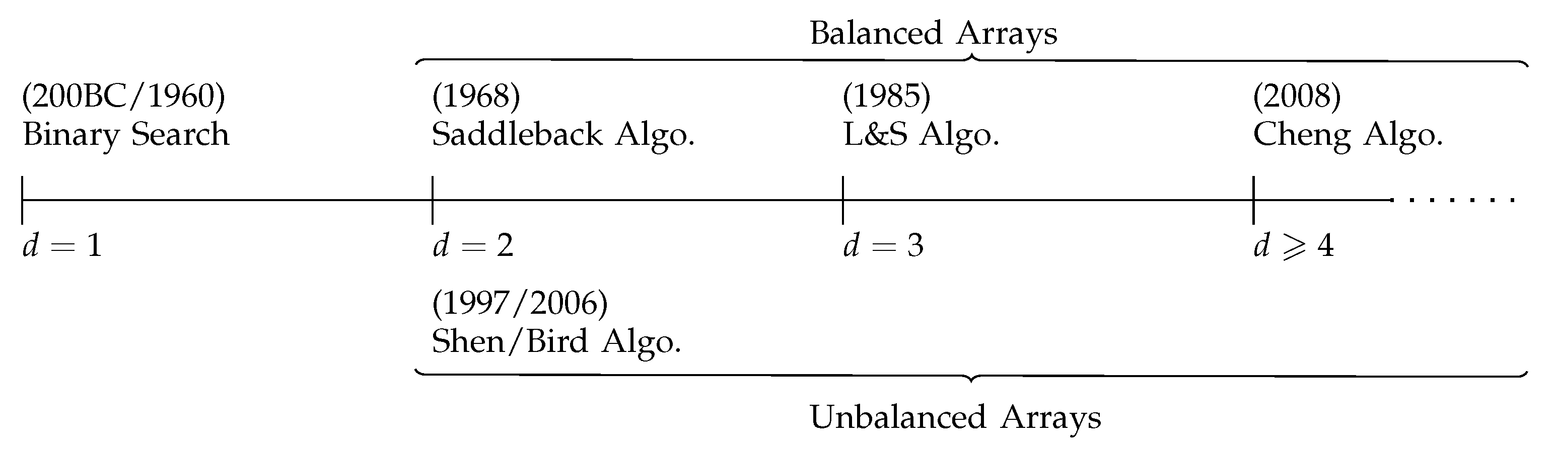
Search efficiency depends upon whether or not A is balanced. A summary of the evolution of the best known search algorithms for the various types of arrays is given in Figure 1.
For 1-dimensional arrays the Binary Search algorithm is worst-case optimal (see Section 3). For balanced 2-dimensional arrays, the Saddleback Search algorithm [1,3,6] is worst-case optimal, and τ ( n , 2 ) is O ( n ) . For unbalanced 2-dimensional arrays there are asymptotically worst case optimal algorithms, and ϕ ( n 1 , n 2 ) is O ( n 2 lg ( n 1 / n 2 ) ) [7,8] (see Section 4).
For the general case of balanced d-dimensional arrays with d 3 , Linial and Saks [5] demonstrated that τ ( n , d ) is O ( n d 1 ) as they proved that
c 2 ( d ) n d 1 + o ( n d 1 ) τ ( n , d ) c 1 ( d ) n d 1 ,
where c 1 ( d ) is a monotone nonincreasing function that is upper bounded by 2 and c 2 ( d ) = ( 24 / π ) d 1 / 2 + o ( d 1 / 2 ) .
Linial and Saks [5] also demonstrated that for the general case of (possibly unbalanced) arrays, with 1 n 1 n 2 n d , ϕ ( n 1 , , n d ) is bounded as follows:
k 2 ( d ) n 1 n d 1 lg ( n d n d 1 + 1 ) ϕ ( n 1 , , n d ) k 1 ( d ) n 1 n d 2 lg ( n d n d 1 + 1 ) ,
where k 1 ( d ) and k 2 ( d ) are functions, with k 1 ( d ) monotone nonincreasing and k 2 ( d ) = c 2 ( d ) k 2 ( d 1 ) / 2 d , and lg ( n ) = log 2 ( n ) . The proofs of the upper bounds on τ ( A ) in the right-hand side of (5) and (
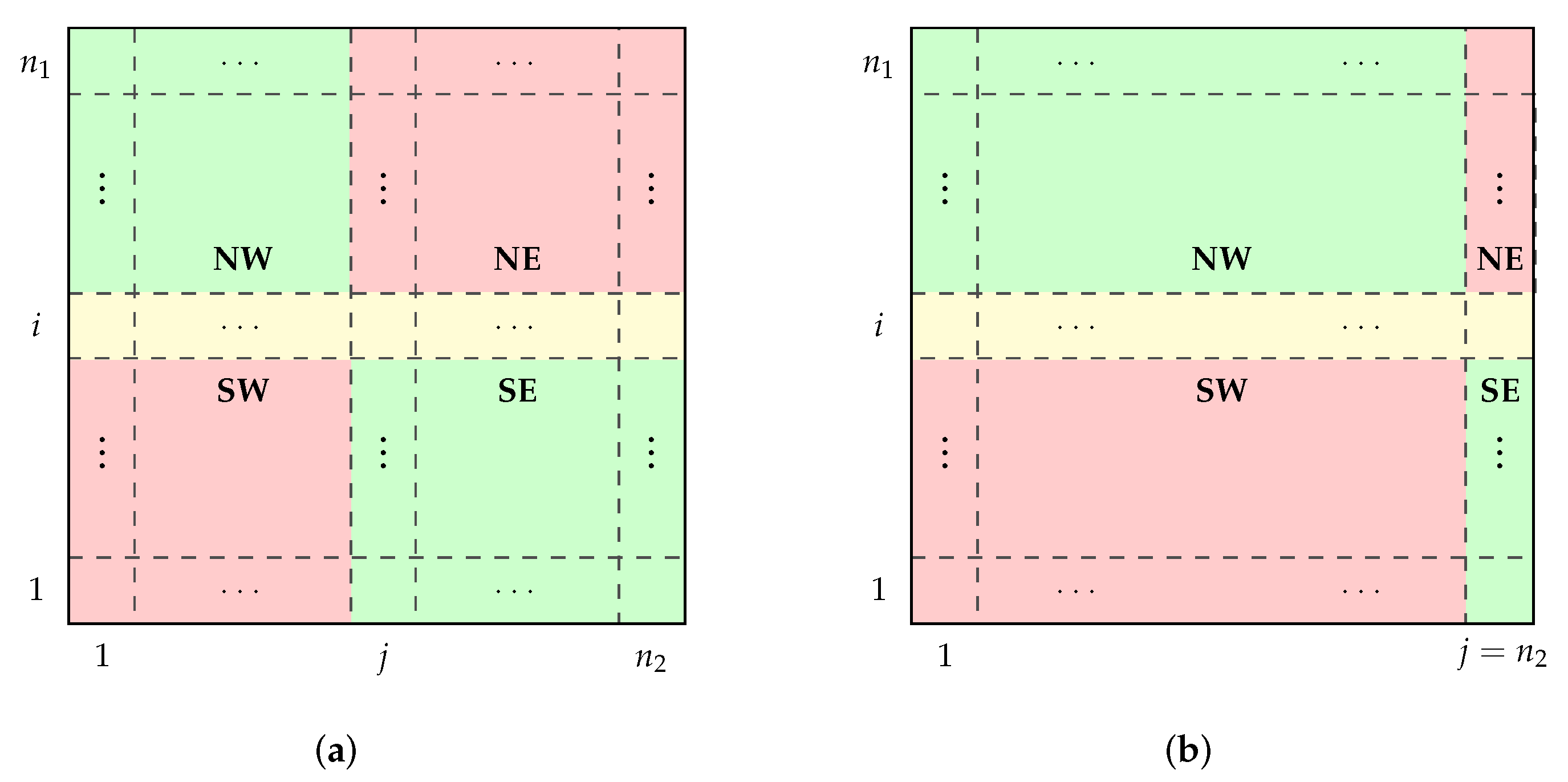
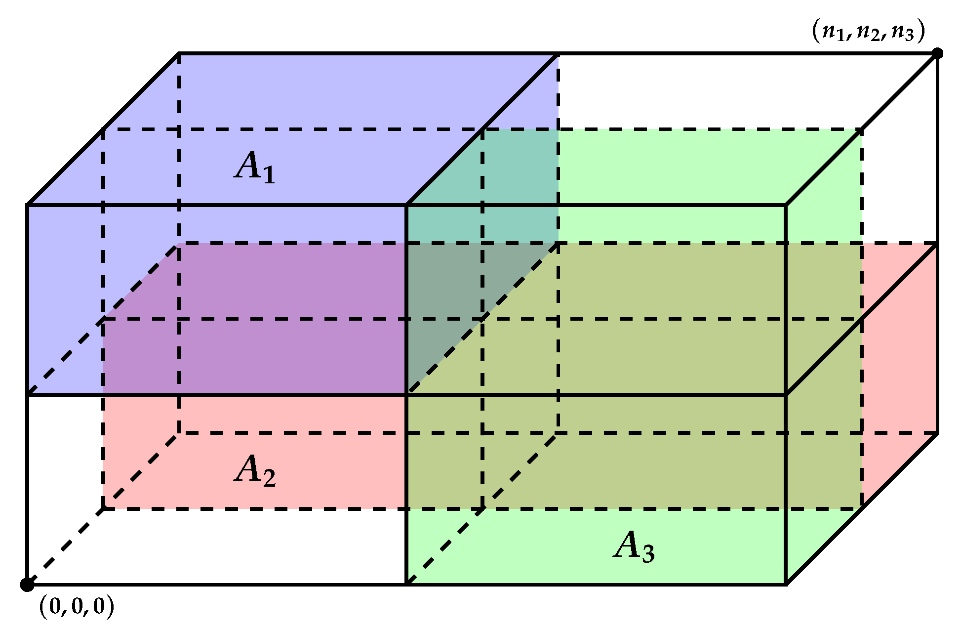
6) were established inductively by the authors by partitioning A into n isomorphic copies of its ( d 1 )-dimensional subarrays, each consisting of all entries that have identical d t h coordinates. The Linial and Saks algorithm [5] for balanced 3-dimensional arrays will be discussed in Section 5.
Cheng et al. [9] proposed an algorithm for d-dimensional hypercubes, for d 4 (see Section 6). Their algorithm has worst case performance upper bounded as follows:
τ ( n , d ) d d 1 n d 1 + O ( n d 2 ) .

3. The Search of Vectors ( d = 1 )

When d = 1 and n 1 = n say, A is a monotone vector (a totally ordered set). Many of the monotone vector search methods mentioned below are based on comparisons of keys and have been described in detail by Knuth [10].
The Linear (or Sequential) Search algorithm (see the pseudocode in Algorithm 1) is a basic method for finding a key within A, whether A is ordered or not. The algorithm starts at the leftmost element of A and iteratively compares the key x with each element of A. The search stops when either x matches an element of A or when all the elements have been tested. Its running time and number of comparisons are, in the worst case, linear in n.
Algorithm 1 LINEAR SEARCH ( A , x )
Input: Array A ( 1 , , n ) and key x R .
Output: True if x A or False otherwise.
   1. i 1 ;
   2. while ( i n ) do
   3.   if ( x = A [ i ] ) then
   4.     return true.
   5.   else
   6.      i i + 1 ;
   7.   end if
   8. end while
   9. return false.
The Jump Search algorithm [11], also known as Block Search [12], check fewer elements of an ordered array A ( 1 , , n ) than the Linear Search, by jumping ahead blocks of a fixed number m of elements. It verifies the elements of A in the indexes 1 , 1 + m , 1 + 2 m , , 1 + k m . Once is determined that A [ 1 + ( k 1 ) m ] < x < A [ 1 + k m ] , a linear search is done in the interval ( 1 + ( k 1 ) m , 1 + k m ) to check if any of these elements is equal the key x. Its pseudocode is shown in Algorithm 2.
Algorithm 2 JUMP SEARCH ( A , x , s t e p )
Input: Array A ( 1 , , n ) and key x R .
Output: True if x A or False otherwise.
  1. i 1 ;
  2. j s t e p + 1 ;
  3. while ( j < n ) and ( A [ j ] < x ) do
  4.     i j ;
  5.     j j + s t e p ;
  6.    if ( j > n ) then
  7.       j n + 1 ;
  8.     end if
  9. end while
10. while  ( i < j )  do
11.       i i + 1 ;
12.      if ( x = A [ i ] ) then
13.   return true.
14.   end if
15. end while
16. return false.
Shneiderman [11] shown that the optimal value of the jump size is m = n . Therefore, if the cost of a jump is c j , and the cost of a sequential search is c s , then the optimum jump size is ( c j / c s ) n and the search cost is τ ( n , 1 ) = ( c j c s ) n . Shneiderman also describes some variations of this algorithm, as the multi-level jumping or the variable jump size.
Jump Search traverses the array back only once, that can be an advantage in situations where jumping back is costly. Note that Binary Search (the next described algorithm), in the worst case, may require up to O ( log n ) back jumps!
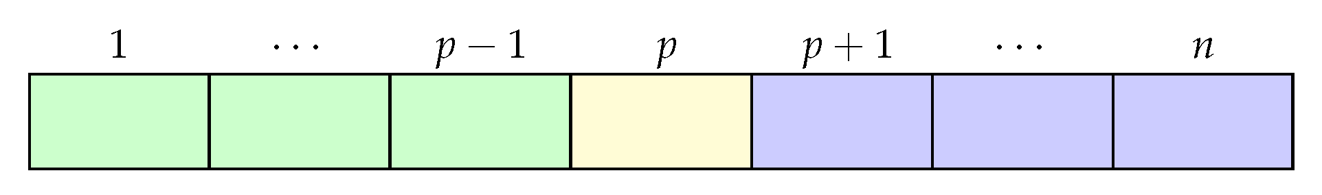
The Binary Search algorithm begins with the vector A as the initial search interval, and repeatedly divides the current search interval into two parts that are either of the same length or differ in length by one unit. If the key x is lower than the entry in the “middle” position of the interval (this situation is depicted in Figure 2, where p is the “middle” position), the search space is narrowed to its lower half (positions 1 to p 1 ). If the key x is greater than the mentioned entry, the interval it is narrowed to the upper half (positions p + 1 to n). The pseudocode of binary search is given in Algorithm 3. It is straightforward to show that the asymptotic complexity of this version of the algorithm is
τ ( n , 1 ) = 2 log ( n ) + 1 = O ( log ( n ) ) .
However, it is not strictly necessary to compare the key x with the element at position p at each iteration of the search loop. An alternative approach, also commonly used, just checks to see if x p . If this is not so, p is returned and the procedure is terminated. Otherwise, p is retained in the search space, which will eventually shrink to p when p = x . However, after exiting the loop, i.e., after the search space is completely exhausted, it is necessary to compare the final element in the space with x. The asymptotic implications of assuming that each iteration requires only one comparison are explored in Section 7.1.
Algorithm 3 BINARY SEARCH ( A , x )
Input: Array A ( 1 , , n ) and key x R .
Output: True if x A or False otherwise.
   1. i 1 ;
   2. j n ;
   3. while ( i j ) do
   4.     p i + j 2 ;
   5.    if ( x = A [ p ] ) then
   6.      return true;
   7.    else if ( x < A [ p ] ) then
   8.       j p 1 ;
   9.    else
 10.       i p + 1 ;
 11.     end if
 12. end while
 13. return false.
The discovery of binary search, also known as logarithmic, divide-and-conquer or bisection search, is attributed by Knuth [10] to Inakibit-Anu of Uruk in 200BC. Binary search was mentioned by Mauchly [13] in what may have been the first published discussion of non-numerical programming methods, but one of the first formal descriptions of it was given by Steinhaus [14]. Furthermore, Sandelius [15] noted that binary search is also optimal in the average case, as cited by Reingold [16].
This history of the evolution of the Binary Search algorithm and its related bibliography, as well as of some other search algorithms listed later here, are described in detail by Knuth [10]. Dijkstra [17] also produced an interesting review of the evolution of the binary search design, from an algorithmic point of view.
Some of these earlier versions of binary search considered only the case where the length of A is a power of 2. At that time the method had become well known, but no one appeared to have reported what should be done to accommodate a general n Z + [15,18,19,20]. It seems that Lehmer [21] was the first to publish a Binary Search algorithm that worked for all n. Lesuisse [22] provides a detailed analysis of various published versions of the binary search algorithm.
In these versions of binary search the position of the central element was calculated and, in the case of fractional values, the position was set to the largest integer smaller than the calculated value. If the sequence contained duplicates of the key value, the first occurrence to the left of the calculated position was found. Bottenbruch [23] presented a variation of the algorithm, that is nowadays most common. Setting the position to the smallest integer greater than or equal to the calculated fractional value, the Bottenbruch algorithm adjusts the left pointer, which initially references the first position of the search, to the next position of the central element whenever the key is greater than or equal to this element. Unlike earlier versions, Bottenbruch’s algorithm finds the rightmost occurrence of a given key when the sequential search identifies duplicate entries of the key. Iverson [24] also proposed a version of binary search for every n Z + , but without considering the possibility of an unsuccessful search. Knuth [25] presented the same algorithm as an example of using an automated system for drawing flowcharts.
Ternary search [26] (also known as dual-pivot binary search [27]) is a divide and conquer algorithm similar to binary search. In this algorithm, the original array is initially divided into three parts of sizes as close as possible to each other. These segments are usually delimited by positions p 1 = 1 + ( n 1 ) / 3 and p 2 = n ( n 1 ) / 3 (see the pseudocode in Algorithm 4). By testing the values at these two positions it is possible to discard 2 3 of the array and proceed with the same approach on the remaining 1 3 of the array. Since a larger portion of the array’s elements are discarded, it may appear that ternary search is faster than binary search. In fact, both algorithms have asymptotic time complexity of O ( lg n ) . However, ternary search uses more comparisons than binary search, which adds greater constants to its asymptotic complexity. Similar arguments are also valid for any other similar higher order search algorithms that are generalised from binary search (i.e. k-nary search, k > 3 ). Section 7.1 provides some detail on the complexity analysis of k-nary search.
Algorithm 4 TERNARY SEARCH ( A , x )
Input: Array A ( 1 , , n ) and key x R .
Output: True if x A or False otherwise.
   1. i 1 ;
   2. j n ;
   3. while ( i j ) do
   4.     p 1 i + ( j i ) 3 ;
   5.     p 2 j ( j i ) 3 ;
   6.    if ( x = A [ p 1 ] ) then
   7.       return true.
   8.     else if ( x = A [ p 2 ] ) then
   9.       return true.
 10.     else if ( A [ p 1 ] > x ) then
 11.         j p 1 1 ;
 12.      else if ( A [ p 2 ] < x ) then
 13.          i p 2 + 1 ;
 14.      else
 15.         i p 1 + 1 ;
 16.         j p 2 1 ;
 17.    end if
 18. end while
 19. return false.
The Interpolation Search algorithm, due to Peterson [28], performs similarly to binary search but unlike it, which always checks the intermediate element of the search space, the interpolation search can check different elements according to the value of the key and the statistical distribution of the elements in the array A. For example, it is likely that the interpolation search will start at an element either near the index n (when the key is closer to A [ n ] ), or near the index 1 (when the key is closer to A [ 1 ] .) The pseudocode is shown in Algorithm 5. When the values in the array A are uniformly distributed, the interpolation search has a performance superior of that of binary search. Perl et al. [29] showed that this algorithm requires on the average log log n array accesses to check if a key is present in the array, assuming that the n array entries are uniformly distributed.
Algorithm 5 INTERPOLATION SEARCH ( A , x )
Input: Array A ( 1 , , n ) and key x R .
Output: True if x A or False otherwise.
   1. i 1 ;
   2. j n ;
   3. while ( i j )   and   ( A [ i ] A [ j ] )   and   ( A [ i ] x A [ j ] ) do
   4.     p i + ( j i ) ( A [ j ] A [ i ] ) · ( x A [ i ] ) ;
   5.    if ( x = A [ p ] ) then
   6.      return true.
   7.    else if ( x < A [ p ] ) then
   8.       j p 1 ;
   9.    else
 10.       i p + 1 ;
 11.    end if
 12. end while
 13. if ( i n ) and ( A [ i ] = x ) then
 14.    return true
 15. else
 16.    return false.
 17. end if
The Exponential Search algorithm is attributed to Bentley and Yao [30]. This search algorithm involves a preliminary step of finding a small range of elements of the array A (potentially containing the key x) and a secondary step of performing a binary search in this limited range of elements. The first step starts with a subarray of size 1, compares its unique element with the key x, then, if necessary, compares a subarray of size 2, then of 4, and so on, until the last element, index i say, of the current subarray is not greater than the key x. At the end of this step, the key can only be present between the indexes i / 2 and i. Therefore, a binary search is carried out in this range. The pseudocode of this algorithm is shown in Algorithm 6. Exponential Search is particularly useful for unbounded arrays, that is, where the size of the array to be searched is infinite. This search also works better than binary search for bounded arrays when the key x is closer to the first element of the array.
Algorithm 6 EXPONENTIAL SEARCH ( A , x )
Input: Array A ( 1 , , n ) and key x R .
Output: True if x A or False otherwise.
   1. i 1 ;
   2. if ( x = A [ i ] ) then
   3.    return true.
   4. end if
   5. while ( i n ) and ( x > A [ i ] ) do
   6.     i i · 2 ;
   7. end while
   8. return BINARY SEARCH ( A ( i 2 + 1 , min { i , n } ) , x ) .
Fibonacci Search (Ferguson [31]) splits the array A into two subarrays with sizes that are consecutive Fibonacci numbers, which are defined as:
F m = m , if 0 m < 2 ; F m 1 + F m 2 , if m 2 .
This search first finds the smallest Fibonacci number, the m t h one say, greater than or equal to n, then uses the ( m 2 ) t h Fibonacci number as the index of the array element to be compared with the key (if it is a valid index). While there are still elements to be inspected, the limits of the subarray that must be searched are calculated based on the three consecutive Fibonacci numbers currently used. The pseudocode shown in Algorithm 7, uses the m t h Fibonacci number just defined and a variable offset to help to discard the unnecessary positions of the array A.
Algorithm 7 FIBONACCI SEARCH ( A , x )
Input: Array A ( 1 , , n ) and key x R .
Output: True if x A or False otherwise.
   1. f F m ;
   2. f 1 F m 1 ;
   3. f 2 F m 2 ;
   4. o f f s e t 0 ;
   5. while ( f > 1 ) do
   6.     p min { o f f s e t + f 2 ; n } ;
   7.    if ( x > A [ p ] ) then
   8.       f f 1 ;
   9.       f 1 f 2 ;
 10.       f 2 f f 1 ;
 11.       o f f s e t p ;
 12.    else if ( x < A [ p ] ) then
 13.       f f 2 ;
 14.       f 1 f 1 f 2 ;
 15.       f 2 f f 1 ;
 16.    else
 17.       return true.
 18.    end if
 19. end while
 20. if  ( f 1 > 0 ) and ( x = A [ o f f s e t + 1 ] ) then
 21.    return true;
 22. else
 23.    return false.
 24. end if

4. The Search of Matrices ( d = 2 )

As illustrated in Figure 3, throughout this survey the corners ( 1 , 1 ) , ( n , 1 ) , ( 1 , n ) and ( n , n ) of 2-dimensional arrays are termed: southwest (SW), northwest (NW), southeast (SE) and northeast (NE) corners, respectively.

4.1. Balanced Matrices

When d = 2 and A is balanced ( n 1 = n 2 = n ), the Saddleback Search algorithm [1,3,6] is worst-case optimal. Saddleback search begins by comparing the key x with the last entry in the first row of A (corner SE in Figure 3). If x is lower than this entry then x cannot be in the column n of A and this column is discarded. If x is greater than this entry then x cannot be in the row 1 of A and this row is discarded. The process is repeated, always comparing x with the last entry in the first row of what remains of A until either x is found or all of the entries of A have been discarded. The pseudocode of the saddleback search is given in Algorithm 8.
A similar argument is valid when x is compared with the last entry in the first column (the corner NW in Figure 3). In fact, at each iteration of the saddleback search either of the entries in the current NW and SE corners can be randomly chosen to be compared with the key x, with the same worst-case performance.
Algorithm 8 SADDLEBACK SEARCH ( A , x )
Input: Array A ( ( 1 , 1 ) , , ( n , n ) ) and key x R .
Output: True if x A or False otherwise.
   1. i 1 ;
   2. j n ;
   3. while ( i n ) and ( j 1 ) do
   4.    if ( x = A ( i , j ) ) then
   5.      return true.
   6. else if ( x > A ( i , j ) )
   7.       i i + 1 ;
   8.   else
   9.       j j 1 ;
 10.   end if
 11. end while
 12. return false.
The above arguments lead to the following result for the worst case performance of saddleback search, according to Graham and Karp, 1968 (quoted in [5]):
τ ( n , 2 ) = 2 n 1 .
The fact that this number is worst case optimal is easily seen through an adversary argument by setting A as:
a ( i , j ) = , if i + j n , + , otherwise .
If any search procedure fails to compare x with any entry a ( i , j ) with i + j = n or i + j = n + 1 (a total of n 1 + n = 2 n 1 entries), then that entry could contain x while still allowing A to be monotone. Thus, any search procedure must make at least 2 n 1 comparisons. Hence, saddleback search is a best possible worst-case procedure. The above argument also holds when A is set as:
a ( i , j ) = , if i + j n + 1 , + , otherwise .

4.2. Unbalanced Matrices

In this section it is assumed that d = 2 and A is unbalanced, i.e., n 1 < n 2 . There is the possibility of searching each of the n 1 rows individually by binary search. This procedure requires O ( n 1 lg ( n 2 ) ) comparisons, which is worst case optimal only if n 1 = o ( n 2 ) [8]. Alternatively, one could divide A into n 2 / n 1 submatrices of dimensions at most n 1 × n 1 and apply saddleback search (as explained in Section 4.1) to each of them. This procedure is worst case optimal only if n 1 = Θ ( n 2 ) . On the other hand, applying saddleback search in the whole matrix lead to a worst case performance of
τ ( n 1 , n 2 ) = n 1 + n 2 1 .
Since A is unbalanced ( n 2 > 6.4 · n 1 , as justified towards the end of Section 4.2.2), none of the aforementioned approaches performs very well in the worst case.
Fortunately, there are search algorithms for unbalanced arrays that are asymptotically worst case optimal, with τ ( n 1 , n 2 ) = O ( n 1 lg ( n 2 / n 1 ) ) [7,8]. These algorithms work by iteratively applying binary search to selected vectors of A to identify pivots. The pivots are used to eliminate redundant entries and to divide the remainder of A into (smaller) subarrays that are searched subsequently. At each iteration, the algorithms eliminate a maximal number of redundant entries.

4.2.1. Shen’s Algorithms

Shen [8] proposed both diagonal-searching and row-searching matrix partitioning algorithms, which are asymptotically worst case optimal for unbalanced arrays. A slightly different algorithm from the latter, which uses linear search instead of binary search in the row-searching step, but achieving the same asymptotic complexity, was proposed previously by Aggarwal et al. [32] in a context of geometric applications.
The pseudocode of Shen’s row-searching procedure is given in Algorithm 9. The algorithm starts by comparing the key x with the two extremes of the middle row of an array A ( ( 1 , 1 ) , , ( n 1 , n 2 ) ) , initially being 1 = 1 , 2 = 1 , r 1 = n 1 and r 2 = n 2 , which has row index i, say. If x < a ( i , 1 ) , the submatrix A ( ( i , 1 ) , , ( n 1 , n 2 ) ) is discarded. If x > a ( i , n 2 ) , the submatrix A ( ( 1 , 1 ) , , ( i , n 2 ) ) is discarded. Otherwise, a binary search on row i generates a pivot a ( i , j ) that allows the submatrices A S W = A ( ( 1 , 1 ) , , ( i , j ) ) and A N E = A ( i , j + 1 ) , , ( n 1 , n 2 ) ) to be discarded. The algorithm proceeds by searching recursively on submatrices A N W = A ( ( i + 1 , 1 ) , , ( n 1 , j ) ) and A S E = A ( ( 1 , j + 1 ) , , ( i 1 , n 2 ) ) . The submatrices A N W , A N E , A S W and A S E are depicted in Figure 4a.
Algorithm 9 SHEN ( A , x )
Input: Array A ( ( 1 , 2 ) , , ( r 1 , r 2 ) ) and key x R .
Output: True if x A or False otherwise.
   1. f o u n d false;
// Stop conditions.  
   2. if ( r 1 1 + 1 < 4 ) or ( r 2 2 + 1 < 4 ) then
   3.    Use BinarySearch in rows/columns; exit;
   4. end if
   5. i 1 + r 1 2 ;
   6. if ( x < a ( i , 2 ) ) then
   7.       f o u n d SHEN( A ( ( 1 , 2 ) , , ( i 1 , r 2 ) ) , x );       // Recursion on submatrix SW-SE.
   8. else if ( x > a ( i , r 2 ) ) then
   9.       f o u n d SHEN( A ( ( i + 1 , 2 ) , , ( r 1 , r 2 ) ) , x );     // Recursion on submatrix NW-NE.
 10. else
 11.       j BinarySearch( A ( ( i , 2 ) , , ( i , r 2 ) ) , x );       // a ( i , j ) x < a ( i , j + 1 ) ?
 12.      if ( x a ( i , j ) ) then
 13.          f o u n d SHEN( A ( ( i + 1 , 2 ) , , ( r 1 , j ) ) , x );         // Recursion on NW.
 14.          f o u n d SHEN( A ( ( 1 , j + 1 ) , , ( i 1 , r 2 ) ) , x );          // Recursion on SE.
 15.      else
 16.          f o u n d True;
 17.      end if
 18. end if
 19. return  f o u n d .
Algorithm 9 has time complexity given by the following recurrences:
ϕ ( n 1 , n 2 ) = O ( lg n 1 ) , if n 2 = 1 ; O ( lg n 2 ) , if n 1 = 1 ; ϕ ( n 1 / 2 , j ) + ϕ ( n 1 / 2 , n 2 j ) + O ( lg ( n 2 ) ) , otherwise .
In the diagonal-searching procedure, Shen’s algorithm [8] divides the n 1 × n 2 matrix A into n 2 n 1 submatrices of dimensions at most n 1 × n 1 and uses binary search to find a pivot element a ( i , j ) on the main diagonal of the “middle” submatrix such that a ( i , j ) < x < a ( i + 1 , j + 1 ) . This pivot splits the matrix into four possible non empty submatrices A N W , A N E , A S W and A S E , as depicted in Figure 4b. Similarly to the row searching schema, the pivot a ( i , j ) allows both submatrices A N E and A S W to be discarded. Therefore, the search only needs to continue on the two matrices A N W = A ( ( i + 1 , 1 ) , , ( n 1 , j ) ) and A S E = A ( ( 1 , j + 1 ) , , ( i , n 2 ) ) of reduced size.
Shen’s diagonal-searching procedure has time complexity given by the following recurrences:
ϕ ( n 1 , n 2 ) = O ( lg n 1 ) , if n 2 = 1 ; O ( lg n 2 ) , if n 1 = 1 ; O ( n 1 ) , if n 1 = n 2 ϕ ( n 1 i , j ) + ϕ ( i , n 2 j ) + O ( lg ( n 2 ) ) , otherwise .
Shen showed that Algorithm 9 has worst case performance when submatrices A N W and A S E have the same size, that is, j = n 2 / 2 . Similarly, in the diagonal-searching procedure the worst case occurs when i = n 1 / 2 . Therefore, given (14) and (15), both algorithms approaches have worst case time complexity of ϕ ( n 1 , n 2 ) = O ( n 1 lg ( 2 n 2 / n 1 ) ) = O ( n 1 lg ( n 2 / n 1 ) ) , which is asymptotically optimal.

4.2.2. Bird’s Algorithm

Bird’s Algorithm [7] uses a row-searching approach that is similar to that of Shen. A binary search is conducted on the middle row of A to find a pivot a ( i , j ) such that a ( i , j ) x < a ( i , j + 1 ) . If x > a ( i , j ) then the search continues only on the two matrices A N E and A S E of reduced size. The algorithm does not perform the two first comparisons of Shen’s Algorithm (Lines 6 and 8), proceeding directly to search in the two submatrices of reduced size (Lines 13 and 14).
Bird provided the following recurrence to express the asymptotic worst case of his algorithm:
ϕ ( n 1 , n 2 ) = O ( lg n 1 ) , if n 2 = 1 ; O ( lg n 2 ) , if n 1 = 1 ; 2 ϕ ( n 1 / 2 , n 2 / 2 ) + O ( lg ( n 2 ) ) , otherwise ;
and hence has time complexity O ( n 1 lg ( n 2 / n 1 ) ) , which is asymptotically optimal.
We now establish an exact count of the number of comparisons required by Bird’s algorithm in the worst case. Suppose that the algorithm is applied to a 2-dimensional n 1 × n 2 array with n 1 n 2 . Since n 1 ( n 2 ) is an integer in a closed range delimited by two consecutive powers of two, the complexity analysis can be done considering that the worst case occurs when n 1 ( n 2 ) is the upper bound of the range, as assumed in the following development:
ϕ ( n 1 , n 2 ) lg n 2 + 2 ϕ ( n 1 / 2 , n 2 / 2 ) = lg n 2 + 2 lg ( n 2 / 2 ) + 2 2 ϕ ( n 1 / 2 2 , n 2 / 2 2 ) = lg n 2 + 2 lg ( n 2 / 2 ) + 2 2 lg ( n 2 / 2 2 ) + + 2 i 1 lg ( n 2 / 2 i 1 ) + 2 i ϕ ( n 1 / 2 i , n 2 / 2 i ) = lg n 2 + 2 ( lg n 2 lg 2 ) + 2 2 ( lg n 2 lg 2 2 ) + + 2 i 1 ( lg n 2 lg 2 i 1 ) + 2 i ϕ ( n 1 / 2 i , n 2 / 2 i ) = lg n 2 k = 0 i 1 2 k k = 0 i 1 k 2 k + 2 i ϕ ( n 1 / 2 i , n 2 / 2 i ) .
When n 1 / 2 i = 1 , n 2 / 2 i > 1 . Thus i = lg n 1 and ϕ ( n 1 / 2 i , n 2 / 2 i ) = ϕ ( 1 , n 2 / 2 lg n 1 ) = ϕ ( 1 , n 2 / n 1 ) = lg ( n 2 / n 1 ) . Then:
ϕ ( n 1 , n 2 ) lg n 2 k = 0 i 1 2 k k = 0 i 1 k 2 k + 2 i ϕ ( n 1 / 2 i , n 2 / 2 i ) = lg n 2 k = 0 lg n 1 1 2 k k = 0 lg n 1 1 k 2 k + 2 lg n 1 lg ( n 2 / n 1 ) = lg n 2 2 lg n 1 1 2 lg n 1 lg n 1 2 lg n 1 2 + 2 + 2 lg n 1 lg ( n 2 / n 1 ) = lg n 2 n 1 1 n 1 lg n 1 2 n 1 + 2 + n 1 lg n 2 n 1 lg n 1 = 2 n 1 lg n 2 2 n 1 lg n 1 lg n 2 + 2 n 1 2 = 2 n 1 lg n 2 2 n 1 lg n 1 + 2 n 1 lg n 2 lg 4 = 2 n 1 lg ( n 2 / n 1 ) + 2 n 1 lg ( 4 n 2 ) .
Thus, Bird’s algorithm has worst case performance
ϕ ( n 1 , n 2 ) = 2 n 1 lg ( n 2 n 1 ) + 2 n 1 lg ( 4 n 2 ) .
A comparison of (13) and (17) leads easily to the following deductions (which also establish the parameter 6.4 as the basis for defining the phrase unbalanced array). If n 1 n 2 6.4 · n 1 , Bird’s algorithm has an inferior worst case performance than that of saddleback search. Conversely, if 6.4 · n 1 < n 2 , and thus the array is unbalanced, the algorithm has a better worst case performance than saddleback search.

4.3. The Location of Pivots when Searching a Row of a 2-d Matrix

The purpose of this subsection is to establish the worst case performance of binary search when it is used as a subroutine to search the middle row of a given 2-dimensional monotone real array A as part of an algorithm that is designed to search A for a given key x. Bird’s algorithm [7] and the first algorithm of Shen [8]) utilise such a subroutine. More specifically, suppose that A n 1 × n 2 with n 1 n 2 , is such a given array and that binary search is applied to the i th row of A, for a given i, 1 i n 1 . That is, the entries, a ( i , q ) , q = 1 , , n 2 ; are to be searched.
We assume from now on that the binary search of row i did not find an instance of the key x, but returned the entry a ( i , j ) ( x ), for some column j of A, 1 j n 2 (see Algorithm 3). In this case a ( i , j ) is used as a pivot by comparing it with x in order to discard the parts of A that now become redundant in the sense that x cannot be a member of them. Let f ( i , j ) be the number elements of A that are thus discarded. The issue to be addressed involves identifying for a given i, which j, where 1 j n 2 , corresponds to the worst case in the sense that using a ( i , j ) as the pivot causes the least number of elements of A, to be discarded. That is, j is worst case if j = argmin f ( i , j ) .
As will be seen later in the present subsection, it has been established that when:
(i)
n 1 is odd, f ( i , j ) is independent of j.
(ii)
n 1 is even and i = n 1 / 2 , f ( i , j ) is minimal when j is maximal.
(iii)
n 1 is even and i = n 1 / 2 + 1 , f ( i , j ) is minimal when j is minimal.
The above results are now investigated in some detail.
If j = 1 ( j = n 2 ), then x < a ( i , q ) ( x > a ( i , q ) ) for q = 1 , , n 2 ; and the rectangle A [ ( i , 1 ) , , ( n 1 , n 2 ) ] ( A [ ( 1 , 1 ) , , ( i , n 2 ) ] ) is redundant and can be discarded. Otherwise, if 1 < j < n 2 , then both x > A [ i , j ] and x < A [ i , j + 1 ] hold and the redundant area comprises the two rectangles: A N E = A [ ( i , j + 1 ) , , ( n 1 , n 2 ) ] and A S W = A [ ( 1 , 1 ) , , ( i , j ) ] . Figure 5a may aid the understanding of the following reasoning. Examples are given in Table 1 and Table 2 in which a zero (unit) entry represents a number less than (greater than) x.
The total number f ( i , j ) of redundant entries defined by the ordered pair of indexes ( i , j ) is:
f ( i , j ) = ( n 1 ( i 1 ) ) n 2 , if j = 1 ; n 2 i , if j = n 2 ; i j + ( n 1 ( i 1 ) ) ( n 2 j ) , if 1 < j < n 2 .
A simple algebraic rearrangement of the case 1 < j < n 2 leads to:
f ( i , j ) = ( n 1 + 1 ) n 2 n 2 i ( n 1 + 1 2 i ) j .
Clearly, the number of entries left to be searched is g ( i , j ) = n 1 n 2 f ( i , j ) , which after some algebraic rearrangement leads to:
g ( i , j ) = ( i 1 ) n 2 , if j = 1 ; ( n 1 i ) n 2 , if j = n 2 ; n 2 i + ( n 1 + 1 2 i ) j n 2 , if 1 < j < n 2 .
Suppose that the middle row of A is searched (as is done in Bird’s algorithm [7] and in the first algorithm of Shen [8]). The special cases when j = 1 or j = n 2 are such that the values of f ( i , 1 ) , g ( i , 1 ) , f ( i , n 2 ) and g ( i , n 2 ) do not depend on the index j and are treated separately at the end of this subsection. We first deal with the case when 1 < j < n 2 and construct the functions f ( i , j ) and g ( i , j ) , on the basis of the parity of n 1 .
  • Case 1 ( n 1 is odd):
The index i is uniquely specified as i = n 1 / 2 and thus i = ( n 1 + 1 ) / 2 . Substituting i in (19), It can be seen that the number of redundant entries reduces to f ( i , j ) = ( n 1 + 1 ) n 2 / 2 , which is independent of j. Thus, it does not matter which entry j of the i th row of A is identified by the binary search as the pivot (including the cases j = 1 and j = n 2 ). Hence, the number g ( i , j ) of entries left to be searched is invariant, where
g ( i , j ) = ( n 1 1 ) n 2 2 .
This case is illustrated in Table 1, where n 1 = 7 , n 2 = 8 , i = 4 , f ( 4 , j ) = 32 and g ( 4 , j ) = 24 , j = 1 , , 8 .
  • Case 2 ( n 1 is even):
The index i can be specified as either i = n 1 / 2 ( i = n 1 / 2 ) or i = n 1 / 2 + 1 ( i = n 1 / 2 + 1 ). For either specification, an obvious task is to identify the column j of A that corresponds to the worst case, where the least number of entries is made redundant. This happens when, for a specified row i, binary search returns an index j corresponding to argmin ( f ( i , j ) ) or, equivalently, to argmax ( g ( i , j ) ). The two specifications of i are now settled.
  • Case 2(a) ( n 1 is even and i = n 1 / 2 ):
It can be seen from (19) that f ( i , j ) reduces to ( n 1 + 2 ) n 2 / 2 j , which is minimal when j is as large as possible ( j = n 2 1 ). Thus, the number of entries left to be searched is
g ( i , j ) = n 1 n 2 2 1 .
This case is illustrated in Figure 5b.
  • Case 2(b) ( n 1 is even and i = n 1 / 2 + 1 ):
Here f ( i , j ) reduces to ( n 1 n 2 ) / 2 + j ) , which is minimal when j is as small as possible, i.e., j = 2 . Thus, the number of entries left to be searched is,
g ( i , j ) = n 1 n 2 2 2 .
Note that for the separate cases when the binary search returns either j = 1 or j = n 2 as the pivot, the number of entries left to be searched is g ( i , n 2 ) = ( n 1 n 2 ) / 2 , which is higher than those in relations (22) and (23). The cases are illustrated in Table 2, where n 1 = 6 and n 2 = 8 . As an example of Case 2( a ), if i = 3 and j = 7 , then f ( 3 , 7 ) = 25 and g ( 3 , 7 ) = 23 . However, if i = 3 and j = 1 , then f ( 3 , 1 ) = g ( 3 , 1 ) = 24 . As an example of Case 2( b ), if i = 4 and j = 2 , then f ( 4 , 2 ) = 26 and g ( 4 , 2 ) = 22 . However, if i = 3 and j = 8 , then f ( 3 , 8 ) = g ( 3 , 8 ) = 24 .

5. Searching the Cuboid ( d = 3 )

5.1. The Balanced Case (the n -Cube)

For the particular case where d = 3 , and the array is balanced (an n -cube), Linial and Saks [5] improved on the bounds in (5) by establishing
3 2 n 2 τ ( n , 3 ) 3 2 n 2 + 3 n lg ( n + 2 ) .
As the authors mention, the lower bound in the left-most expression of (24) can be established as follows. The worst case instance is given by
a ( i , j , k ) = , if i + j + k 3 n / 2 + 1 and n is even ; , if i + j + k 3 n / 2 + 3 / 2 and n is odd ; + , otherwise .
For n even, if any search algorithm fails to compare x with any element a ( i , j , k ) , where:
i + j + k = 3 2 n + 1
or
i + j + k = 3 2 n + 2 ,
then that element could be equal to x even though A is monotone.
For n odd, if any algorithm fails to compare x with any element a ( i , j , k ) , where:
i + j + k = 3 2 n + 3 2
or
i + j + k = 3 2 n + 5 2 ,
then that element could be equal to x even though A is monotone.
It is straightforward to compute the number of elements satisfying (26) and (27). As an illustration, for (26) we must enumerate the number of triples ( i , j , k ) in the range 1 , , n that sum to 3 n / 2 + 1 . To do this, one should count the number of triples for which i , j , k 1 and subtract from it the number of triples for which at least one of i , j , k > n .
The number of triples that sum to 3 n / 2 + 1 is 3 n / 2 2 . The number of triples that sum to 3 n / 2 + 1 with a term bigger than n is 3 n / 2 2 . Thus, the total is 3 n / 2 2 3 n / 2 2 , which is 3 n 2 / 4 .
For the expression in (27) it is necessary to count the number of triples ( i , j , k ) , in the range 1 , , n ; that sum to 3 n / 2 + 2 , which is 3 n / 2 + 1 2 . The number of triples that sum to 3 n / 2 + 2 with a term bigger than n is 3 n / 2 + 1 2 . Hence the total is 3 n / 2 + 1 2 3 n / 2 + 1 2 , which is also 3 n 2 / 4 . Therefore the number of elements satisfying (26) and (27) is 3 n 2 / 2 . The number of elements satisfying (28) and (29) follows analogously, which is 3 n 2 / 2 . Thus the first inequality in (24) is proven.
Linial and Saks [5] established the upper bound in the right-most expression of (24) by constructing an algorithm (termed the L&S Algorithm here) with worst case performance equal to the bound. As the constant of the right-most expression in (24) is positive, the L&S algorithm is asymptotically tight in the worst case. An outline of the algorithm follows. It alternates between applying binary search along a closed path of particular vectors and by applying Saddleback Search described in Section 4.1 for a rectangle, which progressively reduces n by two units at each iteration. At the first stage of the first iteration of the algorithm, binary searches for x are conducted along six vectors that together form what we call the Yellow Brick Road (The Yellow Brick Road is a fictional element in the children’s novel The Wonderful Wizard of Oz by United States author L. Frank Baum (1900)) (YBR) cycle. The simplified diagram in Figure 6a illustrates this cycle, which comprises paths that connect the following entries of A : r = a ( n , n , 1 ) , s = a ( n , 1 , 1 ) , t = a ( n , 1 , n ) , u = a ( 1 , 1 , n ) , v = a ( 1 , n , n ) and w = a ( 1 , n , 1 ) .
The paths of the initial YBR cycle are the vectors that connect the ordered pairs of entries: ( r , s ) , ( s , t ) , ( t , u ) , ( u , v ) , ( v , w ) and ( w , r ) . These paths can be represented as the vectors: a ( n , j 1 , 1 ) , j 1 = 1 , , n , a ( n , 1 , k 1 ) , k 1 = 1 , , n , a ( i 1 , 1 , n ) , i 1 = 1 , , n , a ( 1 , j 2 , n ) , j 2 = 1 , , n , a ( 1 , n , k 2 ) , k 2 = 1 , , n and a ( i 2 , n , 1 ) , i 2 = 1 , , n , respectively.
The binary searches along these paths identify indexes j 1 , k 1 , i 1 , j 2 , k 2 and i 2 , respectively, such that x > v , v { a ( i 1 , n , 1 ) , a ( i 2 , 1 , n ) , a ( 1 , j 1 , n ) , a ( n , j 2 , 1 ) , a ( 1 , n , k 1 ) , a ( n , 1 , k 2 ) } and x < v , v { a ( i 1 + 1 , n , 1 ) , a ( i 2 + 1 , 1 , n ) , a ( 1 , j 1 + 1 , n ) , a ( n , j 2 + 1 , 1 ) , a ( 1 , n , k 1 + 1 ) , a ( n , 1 , k 2 + 1 ) } . The index j 1 allows to discard the two-dimensional subarrays a ( ( 1 , 1 , 1 ) , , ( n , j 1 , 1 ) ) and a ( ( n , i 1 + 1 , 1 ) , , ( n , n , n ) ) . The subarrays discarded via index i 2 are A ( ( 1 , 1 , 1 ) , , ( i 2 , n , 1 ) ) and A ( ( i 2 + 1 , n , 1 ) , , ( n , n , n ) ) , as depicted in the Figure 6b. Each of the other indices, similarly, allows two other two-dimensional subarrays to be discarded.
However, in the worst case, there may remain a subarray of each of the original six faces of A . For example, regarding the indices j 1 and i 2 , there remains the subarray A ( ( i 2 , j 1 , 1 ) , , ( n , n , 1 ) ) within the original face A ( ( 1 , 1 , 1 ) , , ( n , n , 1 ) ) , as depicted in the Figure 6b. In the second stage, the L&S algorithm searches for x in these six subarrays using the adaption of saddleback search for the rectangle. In the worst case, when x is not found by any of these searches, what is left of the original array A is a subarray of dimension ( n 2 ) × ( n 2 ) × ( n 2 ) , to which the algorithm L&S is again applied.
The pseudocode of the L&S algorithm is given in Algorithm 10. The specialized version of the binary search in steps 8 to 13 return both an indication of whether the key was found (or not) and its position in the array (or the position of the first entry greater than the key). The operator ∨ in steps 9 to 13 implies that the algorithm is terminated if one of the binary searches along the YBR path finds x . Similarly, in steps 15 to 20, the search is terminated if one of the calls to the specialized version of the saddleback search finds x .
It is straightforward to show that the L&S algorithm has the following recurrence for the worst-case number of required comparisons needed to search for a key x :
τ ( n , 3 ) τ ( n 2 , 3 ) + 6 lg ( n + 1 ) + 6 ( n 1 ) .
Solving the recurrence (30), establishes the following upper bound on the number of comparisons required by the L&S algorithm [5].
τ ( n , 3 ) 3 n 2 / 2 + 3 n lg ( n + 2 ) .
Algorithm 10 L&S ( A , x )
Input: Array A ( ( 1 , 2 , 3 ) , , ( r 1 , r 2 , r 3 ) ) and key x R .
Output: True if x A or False otherwise.
   1. if ( 1 = r 1 ) and ( a ( 1 , 2 , 3 ) = x )  then                   // Stop conditions
   2.    return true
   3. end if
   4. if ( 1 = r 1 ) and ( a ( 1 , 2 , 3 ) x ) then
   5.    return false.
   6. end if
   7. found false;                        // Stage 1: Search on YBR path.
   8. ( i 1 , found ) BinarySearch( A ( ( 1 , r 2 , 3 ) , , ( r 1 , r 2 , 3 ) ) , x );
   9. ( k 1 , found ) found BinarySearch( A ( ( 1 , r 2 , 3 ) , , ( 1 , r 2 , r 3 ) ) , x );
 10. ( j 1 , found ) found BinarySearch( A ( ( 1 , 2 , r 3 ) , , ( 1 , r 2 , r 3 ) ) , x );
 11. ( i 2 , found ) found BinarySearch( A ( ( 1 , 2 , r 3 ) , , ( r 1 , 2 , r 3 ) ) , x );
 12. ( k 2 , found ) found BinarySearch( A ( ( r 1 , 2 , 3 ) , , ( r 1 , 2 , r 3 ) ) , x );
 13. ( j 2 , found ) found BinarySearch( A ( ( r 1 , 2 , 3 ) , , ( r 1 , r 2 , 3 ) ) , x );
 14. if not found then                      // Stage 2: Search on A sub-faces.
 15.     found SaddlebackSearch( A ( ( i 1 , j 2 , 3 ) , , ( r 1 , r 2 , 3 ) ) , x );
 16.     found found SaddlebackSearch( A ( ( 1 , r 2 , 1 ) , , ( i 1 , r 2 , k 1 ) ) , x );
 17.     found found SaddlebackSearch( A ( ( 1 , j 1 , k 1 ) , , ( 1 , r 2 , r 3 ) ) , x );
 18.     found found SaddlebackSearch( A ( ( 1 , 2 , r 3 ) , , ( i 2 , j 1 , r 3 ) ) , x );
 19.     found found SaddlebackSearch( A ( ( i 2 , 2 , k 2 ) , , ( r 1 , 2 , r 3 ) ) , x );
 20.     found found SaddlebackSearch( A ( ( r 1 , 2 , 3 ) , , ( r 3 , j 2 , k 2 ) ) , x );
 21. end if
 22. if not found then                       // Recursive call of L&S algorithm.
 23.       found L&S( A ( ( 1 + 1 , 2 + 1 , 3 + 1 ) , , ( r 1 1 , r 2 1 , r 3 1 ) ) , x );
 24. end if
 25. return found .
While the L&S algorithm is worst-case optimal, for small arrays it does not necessarily have the best performance. The approach, denoted here by SBS3, is based on partitioning A into n isomorphic copies of its 2-dimensional subarrays, each consisting of all entries that have identical 3rd coordinates. Saddleback search is then used repeatedly to search each 2-dimensional subarray. SBS3 has worst case time complexity of τ ( n , 3 ) 2 n 2 n . This complexity is compared with that of the L&S algorithm τ ( n , 3 ) ( 3 n / 2 + 3 n lg ( n + 2 ) ) in Figure 7. It can be seen that SBS3 is superior when n 33 and the L&S algorithm dominates otherwise.

5.2. The Unbalanced Case (the Cuboid)

Of course, the unbalanced 3-dimensional array, the cuboid, is a special case of the hypercuboid. As given in (37) below, Linial and Saks (Theorem 5.3 in [5]) showed that for n 1 n 2 n d ; the performance ϕ ( n 1 , , n d ) of any search algorithm of the rectangular hypercuboid is bounded above and below by functions of the order of O ( n 1 n d lg ( n 1 / n 2 ) ).
Furthermore, it is possible to extend to cuboids, the search methods for unbalanced 2-arrays of Shen [8] and Bird [7] given in Section 4. For example, such an algorithm extended from one of the Shen’s methods iteratively searches particular cuboids of smaller sizes after discarding entries of the original cuboid A that cannot be x [33]. The algorithm identifies a pivot (the maximum entry that is less than or equal to the key x ) by applying binary search to a particular diagonal of the middle (balanced) 3-dimensional array of maximum possible volume of the current cuboid. Once found, the pivot is used to discard entries of A , if possible, using (1) and (3). The remainder of the cuboid is then divided into three smaller cuboids A 1 , A 2 and A 3 (see Figure 8).
The same process is repeated on these three smaller cuboids, until either x is found or all of the remaining cuboids are one- or two-dimensional subarrays. Binary search is used to explore any remaining vectors and either Bird’s or Shen’s method [7,8] is used for any remaining two-dimensional subarrays. This leads to the recurrence (32), given next. The attainment of exact bounds derived from (32) remains an open problem.
ϕ ( n 1 , n 2 , n 3 ) = 1 , if n 1 = n 2 = n 3 = 1 ; lg ( n 1 + 1 ) , if n 1 > 1 and n 2 = n 3 = 1 ; lg ( n 2 + 1 ) , if n 2 > 1 and n 1 = n 3 = 1 ; lg ( n 3 + 1 ) , if n 3 > 1 and n 1 = n 2 = 1 ; O ( min { n 1 , n 2 } lg ( max { n 1 , n 2 } min { n 1 , n 2 } + 1 ) ) , if n 1 , n 2 > 1 and n 3 = 1 ; O ( min { n 1 , n 3 } lg ( max { n 1 , n 3 } min { n 1 , n 3 } + 1 ) ) , if n 1 , n 3 > 1 and n 2 = 1 ; O ( min { n 2 , n 3 } lg ( max { n 2 , n 3 } min { n 2 , n 3 } + 1 ) ) , if n 2 , n 3 > 1 and n 1 = 1 ; O ( lg ( max { n 1 , n 2 , n 3 } + 1 ) + ϕ ( n 1 , n 2 / 2 , n 3 / 2 ) + ϕ ( n 1 / 2 , n 2 , n 3 / 2 ) + ϕ ( n 1 / 2 , n 2 / 2 , n 3 ) , otherwise .

6. Searching in Higher Dimensions ( d 4 )

6.1. Balanced Case (Hypercubes)

Cheng et al [9] extended the results of Linial and Saks [5] for the cube, described in Section 5, to d -dimensional hypercubes for d 4 . The Cheng et al. algorithm is described as a generalization of a particular algorithm (which we call Cheng-4) for the special case d = 4 . The authors use the lower bound 4 / 3 n 3 n / 3 τ ( n , 4 ) to the Cheng-4 algorithm, which they showed to be asymptotically tight.
Cheng-4 first selects eight particular 2- d outer faces of the 4- d hypercube A and uses an adaptation of the saddleback search to partition each of these eight 2- d arrays into two surfaces, requiring at most 8 ( 2 n 1 ) tests. These surfaces generate eight 3- d subarrays of A that are then searched with at most 8 n 2 tests. Similarly to the L&S algorithm this process reduces the remaining 4- d hypercube to be searched to one with sizes ( n 2 ) . The authors established that, for n > 2 , the worst case performance of their algorithm is given by
τ ( n , 4 ) τ ( n 2 , 4 ) + 8 n 2 + 8 ( 2 n 1 ) .
This recurrence implies that τ ( n , 4 ) 4 / 3 n 3 + O ( n 2 ) . Therefore, using their lower bound the authors have shown that
4 / 3 n 3 n / 3 τ ( n , 4 ) 4 / 3 n 3 + O ( n 2 ) ,
and that the algorithm is asymptotically optimal up to the lower order terms.
The partition of each one of the eight 2- d outer faces of the 4- d hypercube generates two subsets S and L , such that S contains entries smaller than x and L contains entries larger than x . These subsets are derived from two 2-dimensional arrays u and v , each containing n integers such that i 1 u [ i 2 ] iff a ( i 1 , i 2 ) < x and i 2 v [ i 1 ] iff a ( i 1 , i 2 ) < x . The sets S and L , as well as the arrays u and v are illustrated in Figure 9.
The eight 2- d outer faces are defined by fixing a pair of subscripts ( i p , i q ) , p = 1 , , 4 and q = ( p + 1 ) mod 4 , to either ( 1 , n ) or ( n , 1 ) and are denoted by M i and M i * , i = 1 , , 4 . For example, M 1 is obtained by the indexes a ( i 1 , i 2 , 1 , n ) , i 1 , i 2 = 1 , , n , and generates the partitions S 1 and L 1 . Similarly, M 1 * = { a ( i 1 , i 2 , n , 1 ) } , i 1 , i 2 = 1 , , n , generates S 1 * and L 1 * .
Using some properties as to whether or not the key belongs to the 2- d partitions, eight 3- d surfaces Q i = { a ( i 1 , i 2 , i 3 , i 4 ) } and Q i * = { a ( j 1 , j 2 , j 3 , j 4 ) } are defined, by fixing i k = 1 and j k = n for k = 1 , , 4 . The search then proceeds in some subarrays of these eight surfaces generated by the intersections induced by the partitions S i and L i ( S i * and L i * ). An example of these intersections is depicted in Figure 10. For further details the reader is referred to [9].
Cheng et al. [9] also showed how the algorithm Cheng-4 can be generalised to d -dimensional hypercubes, for d 5 , in a straightforward way. As with Cheng-4, the search is carried out in two steps. In the first step, the algorithm partitions the original matrix A n , d into 2 d subsets S k and L k , k = 1 , , d ; such that S k contains entries smaller than x and L k contains entries larger than x . The algorithm considers 2 d ( d 2 ) -dimensional arrays as defined below:
M k = { a ( i 1 , i 2 , , i d ) i k 2 = 1 , i k 1 = n } S k , L k , M k * = { a ( i 1 , i 2 , , i d ) i k 2 = n , i k 1 = 1 } S k * , L k * .
The aim of using the subsets S k and L k is to attempt to eliminate part of the surface of a particular subarray by fixing ( d 3 ) subscripts.
The d pairs of “mutually complementary” subsets ( S k , L k ) and ( S k * , L k * ) ( k = 1 , , d ) have the following properties:
(a)
x > a ( i 1 , , i d i ( k 2 ) mod d = 1 , i ( k 1 ) mod d = n ) and x < a ( j 1 , , j d ) j ( k 2 ) mod d = 1 , j ( k 1 ) mod d = n ) for ( i k , , i k + d 3 ) S k and ( j k , , j k + d 3 ) L k ,
(b)
x > a ( i 1 , , i d i ( k 2 ) mod d = n , i ( k 1 ) mod d = 1 ) and x < a ( j 1 , , j d ) j ( k 2 ) mod d = n , j ( k 1 ) mod d = 1 ) for ( i k , , i k + d 3 ) S k * and ( j k , , j k + d 3 ) L k * ,
for all k = 1 , , d .
In total, the first step produces 4 d ( d 3 ) -dimensional arrays. At most 2 n 1 comparisons are needed for each fixed subscript i 2 , , i d 3 and hence at most 2 dn d 4 ( 2 n 1 ) comparisons in total are required.
In the second step, the surfaces of the subarrays are searched in order to reduce the region of uncertainty to a d -dimensional array with sizes at most ( n 2 ) . The algorithm searches the following 2 d ( d 1 ) -dimensional surfaces of A n , d , that are defined by fixing one of the subscripts at either 1 or n :
Q k = { a ( i 1 , , i d ) i k = 1 } , Q k * = { a ( i 1 , , i d ) i k = n } , k = 1 , , d .
In total, the second step requires at most 2 dn d 2 comparisons.
Steps 1 and 2 reduce the original array to a d -dimensional array A n 2 , d , with sizes of at most ( n 2 ) . That is,
A n 2 , d = { a i 1 , , i d i 1 , , i d = 2 , , n 1 } .
Hence the generalised recursion is:
τ ( n , d ) 1 , if n = 1 ; 2 d , if n = 2 ; τ ( n 2 , d ) + 2 dn d 2 + 2 dn d 4 ( 2 n 1 ) , for n > 2 .
Solving this recursion leads to a worst case performance of the algorithm of
τ ( n , d ) d d 1 n d 1 + O ( n d 2 ) , d 4 .

6.2. Unbalanced Case (the Hypercuboids)

For the general case of a d -dimensional array that is not necessarily balanced, Linial and Saks [5] proved that, for n 1 n 2 n d ; there exists a nonincreasing function k 1 ( d ) and a function k 2 ( d ) such that the performance ϕ ( n 1 , , n d ) of any search algorithm is bounded as follows:
k 2 ( d ) n 1 n d 1 lg ( n d n d 1 + 1 ) ϕ ( n 1 , , n d ) k 1 ( d ) n 1 n d 2 lg ( n d n d 1 + 1 ) ,

7. The Worst Case Performance of Some of the Revised Algorithms

From (8), the binary search of a sorted one-dimensional array of size n can be performed with log ( n ) + 1 comparisons in the worst case. However, there is some justification in assuming that using (1), (2) and (3) at each iteration of such a binary search actually requires two comparisons (not one). Some implications of making such an assumption are now established.

7.1. Binary and k -Nary Search Revised

The worst case performance of the binary search version that uses only one comparison at each iteration, as described in Section 3, can be stated as follows:
τ ( n , 1 ) 1 , if n = 1 ; 1 + τ ( n / 2 , 1 ) , otherwise .
Therefore,
τ ( n , 1 ) 1 + τ ( n / 2 , 1 ) = 1 + 1 + τ ( n / 2 / 2 , 1 ) = 1 + + 1 i + τ ( n / 2 / 2 i 1 , 1 ) = 1 + + 1 i + τ ( n / 2 i , 1 ) = i + τ ( n / 2 i , 1 ) .
When n / 2 i = 1 , τ ( n / 2 i , 1 ) = τ ( 1 , 1 ) = 1 . Moreover,
n / 2 i = 1 1 n / 2 i < 2 2 i n < 2 i + 1 lg 2 i lg n < lg 2 i + 1 i lg n < i + 1 i = lg n .
Thus,
τ ( n , 1 ) lg n + 1 .
This result can be generalised to k -nary versions of the algorithm, i.e., that divide the search space into k parts, as follows:
τ ( n , 1 ) c k , if n < k ; b k + τ ( n / k , 1 ) , otherwise ;
where c k is a tight upper bound on the number of comparisons necessary to check the elements still eventually remaining after exiting the search loop and b k expresses the complexity of dividing the search space into k parts, defined by k 1 pivot elements, and the necessary comparisons of the key x with those pivot elements. Thus,
τ ( n , 1 ) b k log k n + c k .
Thus, as k increases, the logarithm basis and the constants c k and b k also increase since more operations are necessary to determine in which subspace to continue the search. Therefore, in practice, the gain of performance obtained by increasing the logarithm basis is practically cancelled out by increasing the constants c k and b k .

7.2. Shen’s Algorithm Revised

We now establish a revised exact count of the number of comparisons required by the Shen’s row search algorithm [8] in the worst case. The worst possible location of the pivot on the “middle” row of the matrix, discussed in Section 4.3, leads to the following revised recurrence relation for the algorithm:
ϕ ( n 1 , n 2 ) 1 , if n 2 = n 1 = 1 ; 2 lg n 2 + 1 , if n 2 > 1 and n 1 = 1 ; 2 lg n 1 + 1 , if n 2 = 1 and n 1 > 1 ; ( 2 lg n 2 + 1 ) + ( 2 lg ( n 1 / 2 1 ) + 1 ) + ϕ ( n 1 / 2 , n 2 1 ) , otherwise .
Note ( x = k k x < k + 1 and x = k k 1 < x k .) that n 1 / 2 i n 1 / 2 i 1 n 1 / 2 i 1 n 1 / 2 i . Moreover, lg n 1 / 2 lg n 1 / 2 . Thus:
ϕ ( n 1 , n 2 ) ( 2 lg n 2 + 1 ) + ( 2 lg ( n 1 / 2 1 ) + 1 ) + ϕ ( n 1 / 2 , n 2 1 ) ( 2 lg n 2 + 1 ) + ( 2 lg ( n 1 / 2 ) + 1 ) + ϕ ( n 1 / 2 , n 2 1 ) = [ ( 2 lg n 2 + 1 ) + ( 2 lg ( n 2 1 ) + 1 ) ] + [ ( 2 lg ( n 1 / 2 ) + 1 ) + ( 2 lg ( n 1 / 2 2 ) + 1 ) ] + ϕ ( n 1 / 2 2 , n 2 2 ) = [ ( 2 lg n 2 + 1 ) + ( 2 lg ( n 2 1 ) + 1 ) + + ( 2 lg ( n 2 ( i 1 ) ) + 1 ) ] + [ ( 2 lg ( n 1 / 2 ) + 1 ) + ( 2 lg ( n 1 / 2 2 ) + 1 ) + + ( 2 lg ( n 1 / 2 i ) + 1 ) ] + ϕ ( n 1 / 2 i , n 2 i ) .
Observe that n 1 / 2 i n 1 / 2 i lg ( n 1 / 2 i ) lg ( n 1 / 2 i ) = lg n 1 lg 2 i = lg n 1 i . Therefore,
ϕ ( n 1 , n 2 ) [ ( 2 lg n 2 + 1 ) + ( 2 lg ( n 2 1 ) + 1 ) + + ( 2 lg ( n 2 ( i 1 ) ) + 1 ) ] + [ ( 2 lg ( n 1 / 2 ) + 1 ) + ( 2 lg ( n 1 / 2 2 ) + 1 ) + + ( 2 lg ( n 1 / 2 i ) + 1 ) ] + ϕ ( n 1 / 2 i , n 2 i ) = 2 k = 0 i 1 lg ( n 2 k ) + i + 2 k = 0 i ( lg n 1 lg 2 k ) + i + ϕ ( n 1 / 2 i , n 2 i ) . [ 2 i lg n 2 + i ] + 2 k = 0 i ( lg n 1 k ) ) + i + ϕ ( n 1 / 2 i , n 2 i ) [ 2 i lg n 2 + i ] + [ 2 ( i + 1 ) lg n 1 ( 1 + + i ) + i ] + ϕ ( n 1 / 2 i , n 2 i ) = [ 2 i lg n 2 + i ] + [ 2 ( i + 1 ) lg n 1 i 2 ] + ϕ ( n 1 / 2 i , n 2 i ) [ 2 i lg n 2 + i ] + [ 2 ( i + 1 ) lg n 1 i 2 ] + ϕ ( n 1 / 2 i , n 2 i )
There are two cases to be considered:
  • n 1 / 2 i = 1 and n 2 i > 1 , then i lg n 1 and ϕ ( n 1 / 2 i , n 2 i ) ϕ ( 1 , n 2 lg n 1 ) 2 lg ( n 2 lg n 1 ) + 1 2 lg ( n 2 lg n 1 ) + 1 . Then,
    ϕ ( n 1 , n 2 ) [ 2 lg n 1 lg n 2 + lg n 1 ] + [ 2 ( lg n 1 + 1 ) lg n 1 ( lg n 1 ) 2 ] + [ 2 lg ( n 2 lg n 1 ) + 1 ] = 2 lg ( n 2 lg n 1 ) + lg n 1 ( 2 lg n 2 + 3 ) + ( lg n 1 ) 2 .
  • n 1 / 2 i > 1 and n 2 i = 1 , then i = n 2 1 and ϕ ( n 1 / 2 i , n 2 i ) ϕ ( n 1 / 2 2 n , 1 ) 2 lg ( n 1 / 2 2 n ) + 1 = 2 lg n 1 n 2 + 1 2 ( lg n 1 n 2 ) + 1 . Then,
    ϕ ( n 1 , n 2 ) [ 2 ( n 2 1 ) lg n 2 ( n 2 1 ) ] + [ 2 ( ( n 2 1 ) + 1 ) lg n 1 ( n 2 1 ) 2 ] + 2 lg n 1 2 n 2 + 1 = 2 n 2 lg ( n 1 n 2 ) + 2 lg n 1 lg n 2 ( n 2 2 n 2 + 1 ) .

7.3. Bird’s Algorithm Revised

We now establish a revised exact count of the number of comparisons required by Bird’s algorithm [7] in the worst case. Suppose that the algorithm is applied to a two-dimensional n 1 × n 2 array with n 1 < n 2 . Suppose further, that when a binary search subroutine is called as a part of the algorithm it has worst case performance given in Equation (39). Then, following the reasoning used to derive Equation (17), it can be established that the worst case performance for the revised Bird’s algorithm is
ϕ ( n 1 , n 2 ) = 4 n 1 lg n 2 n 1 + 6 n 1 2 lg ( 4 n 2 ) .
Note that the count in (43) is significantly higher than that in (17). Recall that from (13), the worst case performance of the adaption of saddleback search for the array under study has a worst case performance of ( n 1 + n 2 1 ) . However, if it is still assumed that two comparisons are necessary at each iteration of saddleback search, then its worst case performance is
ϕ ( n 1 , n 2 ) = 2 ( n 1 + n 2 ) + 1 .
A comparison of Equations (43) and (44) imply that if n 1 n 2 < 8 n 1 , Bird’s algorithm has an inferior worst case performance than that of adapted saddleback search. Conversely, if n 2 8 n 1 , the algorithm has a better worst case performance than revised saddleback search.

7.4. The L&S Algorithm Revised

We now establish a revised exact count of the number of comparisons required by the L&S algorithm in the worst case. Suppose that the algorithm is applied to an n -cube. Suppose further, that when a binary search subroutine is called as a part of the algorithm it has the worst case performance given in Equation (39). Then, following the reasoning used to derive Equation (31), it can be established that the worst case performance for the revised L&S algorithm is
τ ( n , 3 ) 3 n 2 / 2 + 6 n lg ( n + 1 ) + 3 n + 12 lg ( n + 1 ) + 6 .
Note that the count in (45) is significantly higher than that in (31).

8. Searching for All Occurrences of the Key

We now briefly discuss the extended problem of searching for all occurrences of the key. To be meaningful, A must be redefined as a strictly monotone array, i.e., its entries either strictly decrease or strictly increase when moving away from the origin along any path parallel to an axis.
When d = 1 , binary search is the basis for efficiently solving some variants of the search problem, such as determining the index of: ( i ) the first occurrence of the key, ( ii ) the last occurrence of the key, or ( iii ) the least element greater than the key, or ( iv ) the greatest element less than the key. Some minor changes to the basic logic of the Binary Search algorithm are enough to solve variants ( i )–( iv ). A simple combination of the algorithms that solve variants ( i ) and ( ii ) or of those that solve variants ( iii ) and ( iv ) can be used to determine all occurrences of the key.
Regarding the case d = 2 , although it was included as an “existence” method, Bird’s algorithm [7] was actually designed to search for all occurrences of the key.
For the case d 3 , the possibility searching for all occurrences of the key is not discussed in any of the articles cited in the present work. However, certainly, the aforementioned algorithms designed to search for a single instance of the key when d 3 can be extended to search for all occurrences of the key, probably with an increase in complexity.

9. Conclusions

The problem of sequentially searching a real d -dimensional ( d 1 ) array for a given key has been extensively investigated. The formal definition of the problem has been revised and algorithms identified in the specialised literature for it and some of its special cases, including those where the array has sizes not necessarily equal, have been described in detail. Many aspects of algorithm performance complexity have also been discussed. The known d -dimensional (balanced and unbalanced) array search algorithms with the best performing complexities in the worst case are shown in Table 3 for 1 d 4 . It can be seen from the table that each algorithm has order strictly less than a product of the sizes of the array, except for the d = 2 balanced case.
A present challenge is to solve recurrences such as the one in (32). Open problems include those of finding efficient algorithms for d -dimensional unbalanced arrays with d 3 .

Author Contributions

Conceptualization, L.R.F. and H.J.L.; Data curation, M.R.C.; Formal analysis, M.R.C. and L.R.F.; Funding acquisition, M.R.C.; Investigation, L.R.F. and H.J.L.; Methodology, M.R.C., L.R.F. and H.J.L.; Project administration, M.R.C.; Software, M.R.C. and H.J.L.; Supervision, H.J.L.; Validation, M.R.C. and L.R.F.; Visualization, H.J.L.; Writing—original draft, L.R.F. and H.J.L.; Writing—review & editing, M.R.C., L.R.F. and H.J.L. All authors have read and agreed to the published version of the manuscript.

Funding

The authors are grateful to the Fundação de Amparo à Pesquisa do Estado de Goiás-FAPEG-Brazil, for its support of this research (Call 03/2015).

Institutional Review Board Statement

Not applicable.

Informed Consent Statement

Not applicable.

Conflicts of Interest

The authors declare no conflict of interest.

References

  1. Baase, S.; Gelder, A.V. Computer Algorithms: Introduction to Design and Analysis, 3rd ed.; Addison-Wesley: Reading, MA, USA, 2000. [Google Scholar]
  2. Cosnard, M.; Duprat, J.; Ferreira, A. Complexity of selection in X+Y. Theor. Comput. Sci. 1989, 67, 115–120. [Google Scholar] [CrossRef] [Green Version]
  3. Gries, D. The Science of Programming; Texts and Monographs in Computer Science; Springer: Berlin, Germany, 1981. [Google Scholar]
  4. Sarnath, R.; He, X. Efficient parallel algorithms for selection and searching on sorted matrices. In Parallel Processing Symposium, International; IEEE Computer Society: Washington, DC, USA, 1992; pp. 108–111. [Google Scholar] [CrossRef]
  5. Linial, N.; Saks, M. Searching ordered structures. J. Algorithms 1985, 6, 86–103. [Google Scholar] [CrossRef]
  6. Dijkstra, E.W. A Discipline of Programming, 1st ed.; Prentice-Hall, Inc.: Upper Saddle River, NJ, USA, 1976. [Google Scholar]
  7. Bird, R.S. Improving saddleback search: A lesson in algorithm design. In Proceedings of the Mathematics of Program Construction: 8th International Conference, MPC 2006, Lecture Notes in Computer Science. Kuressaare, Estonia, 3–5 July 2006; Uustalu, T., Ed.; Springer: Berlin/Heidelberg, Germany, 2006; Volume 4014, pp. 82–89. [Google Scholar] [CrossRef]
  8. Shen, H. Optimal algorithms for generalized searching in sorted matrices. Theor. Comput. Sci. 1997, 188, 221–230. [Google Scholar] [CrossRef] [Green Version]
  9. Cheng, Y.; Sun, X.; Yin, Y.L. Searching monotone multi-dimensional arrays. Discret. Math. 2008, 308, 2213–2224. [Google Scholar] [CrossRef] [Green Version]
  10. Knuth, D.E. The Art of Computer Programming: Sorting and Searching, 1st ed.; Addison-Wesley Series in Computer Science and Information Processing; Addison-Wesley Pub. Co.: Boston, MA, USA, 1973; Volume 3. [Google Scholar]
  11. Shneiderman, B. Jump Searching: A Fast Sequential Search Technique. Commun. ACM 1978, 21, 831–834. [Google Scholar] [CrossRef]
  12. Martin, J. Computer Data-Base Organization, 2nd ed.; Prentice-Hall Series in Automatic Computation; Prentice-Hall: Englewood Cliffs, NJ, USA, 1977. [Google Scholar]
  13. Mauchly, J.W. Sorting and collating. In Theory and Techniques for the Design of Electronic Digital Computers; Patterson, G.W., Ed.; University of Pennsylvania: Cambridge, MA, USA, 1946; Volume 3, Lecture 22. [Google Scholar]
  14. Steinhaus, H. Mathematical Snapshots, 3rd ed.; Oxford University Press: Oxford, UK, 1960. [Google Scholar]
  15. Sandelius, M. On an optimal search procedure. Am. Math. Mon. 1961, 68, 133–134. [Google Scholar] [CrossRef]
  16. Reingold, E.M. Establishing lower bounds on algorithms: A survey. In Proceedings of the Spring Joint Computer Conference, Atlantic City, NJ, USA, 16–18 May 1972; ACM: New York, NY, USA, 1972; pp. 471–481. [Google Scholar] [CrossRef]
  17. Dijkstra, E.W. EWD1293—Constructing the Binary Search Once More. Department of Computer Sciences, The University of Texas at Austin: Austin, TX, USA. Available online: http://www.cs.utexas.edu/users/EWD/ewd12xx/EWD1293.PDF (accessed on 23 December 2021).
  18. Dumey, A.I. Indexing for rapid random access memory systems. Comput. Autom. 1956, 5, 6–9. [Google Scholar]
  19. Halpern, M. Variable-width tables with binary-search facility. Commun. ACM 1958, 1, 1–3. [Google Scholar] [CrossRef]
  20. McCracken, D.D. Digital Computer Programming; General Electric Series; John Wiley & Sons: New York, NY, USA, 1957. [Google Scholar]
  21. Lehmer, D.H. Teaching combinatorial tricks to a computer. In Combinatorial Analysis; American Mathematical Society: Providence, RI, USA, 1960; pp. 179–193. [Google Scholar]
  22. Lesuisse, R. Some Lessons Drawn from the History of the Binary Search Algorithm. Comput. J. 1983, 26, 154–163. [Google Scholar] [CrossRef]
  23. Bottenbruch, H. Structure and Use of ALGOL 60. J. ACM 1962, 9, 161–221. [Google Scholar] [CrossRef]
  24. Iverson, K.E. A Programming Language; John Wiley & Sons, Inc.: New York, NY, USA, 1962. [Google Scholar]
  25. Knuth, D.E. Computer-drawn Flowcharts. Commun. ACM 1963, 6, 556–558. [Google Scholar] [CrossRef]
  26. Hesselink, W.H. whh303—Ternary Search. Dept. of Mathematics and Computing Science, Rijksuniversiteit Groningen: Groningen, The Netherlands. Available online: http://wimhesselink.nl/pub/whh303.pdf (accessed on 23 December 2021).
  27. Kostyukov, V. Dual-Pivot Binary Search. 2014. Available online: https://kostyukov.net/posts/dual-pivot-binary-search/ (accessed on 4 December 2021).
  28. Peterson, W.W. Addressing for Random-Access Storage. IBM J. Res. Dev. 1957, 1, 130–146. [Google Scholar] [CrossRef]
  29. Perl, Y.; Itai, A.; Avni, H. Interpolation Search—A loglogN Search. Commun. ACM 1978, 21, 550–553. [Google Scholar] [CrossRef]
  30. Bentley, J.L.; Yao, A.C.C. An almost optimal algorithm for unbounded searching. Inf. Process. Lett. 1976, 5, 82–87. [Google Scholar] [CrossRef] [Green Version]
  31. Ferguson, D.E. Fibonaccian Searching. Commun. ACM 1960, 3, 648. [Google Scholar] [CrossRef]
  32. Aggarwal, A.; Klawe, M.; Moran, S.; Shor, P.; Wilber, R. Geometric Applications of a Matrix Searching Algorithm. In Proceedings of the Second Annual Symposium on Computational Geometry; Association for Computing Machinery: New York, NY, USA, 1986; pp. 285–292. [Google Scholar] [CrossRef]
  33. Cappelle, M.R.; Foulds, L.R.; Longo, H.J. A note on searching sorted unbalanced three-dimensional arrays. arXiv 2017, arXiv:1712.02371. [Google Scholar]
Figure 1. The best known algorithms for searching monotone arrays.
Algorithms 15 00010 g001
Figure 2. Binary search vector bisection.
Algorithms 15 00010 g002
Figure 3. Subarray elimination schemes in the saddleback algorithm. (a) Row elimination. (b) Column elimination.
Algorithms 15 00010 g003
Figure 4. The two searching schemes in the algorithm of Shen. (a) The row searching scheme. (b) The diagonal searching scheme.
Algorithms 15 00010 g004
Figure 5. The location of pivots when searching a row. (a) General row search. (b) Row search Case 2(i).
Algorithms 15 00010 g005
Figure 6. An example of a remaining subarray after searching part of the YBR path. (a) The “Yellow Brick Road”. (b) The remaining subarray (the green area).
Algorithms 15 00010 g006
Figure 7. A comparison of the worst case performance of the SBS3 and L&S algorithms.
Algorithms 15 00010 g007
Figure 8. Partition of A into A 1 , A 2 , and A 3 .
Algorithms 15 00010 g008
Figure 9. Partition of a monotone two-dimensional array A n , 2 corresponding to an outer 2- d face of A 4- d hypercube. Adapted from Cheng et al. (a) Vector u and partitions S and L . (b) Vector v and partitions S and L . [9].
Algorithms 15 00010 g009
Figure 10. Searching in the three-dimensional surface Q 1 = { a 1 , i 2 , i 3 , i 4 } of A n , 4 . Adapted from Cheng et al. (a) Partition of M 2 * = { a 1 , i 2 , i 3 , n } into S 2 * and L 2 * . (b) Partition of M 3 = { a 1 , n , i 3 , i 4 } into S 3 and L 3 . (c) The “inverted pyramid” composed of a sequence of three-dimensional matrices to be searched. [9].
Algorithms 15 00010 g010
Table 1. Case 1. n 1 is odd.
Row iColumn j
12345678
711111111
611111111
511111111
400000000
300000000
200000000
100000000
Table 2. Cases 2 (a) and 2(b). n 1 is even with (a) i = 3 and (b) i = 4 .
Row iColumn j
12345678
611111111
511111111
411111111
300000000
200000000
100000000
Table 3. Search algorithms and their worst case performance bounds.
dStructureMethodWorst-Case Complexity
1Binary Search O ( lg ( n ) )
2BalancedSaddleback Search O ( n )
UnbalancedBird/Shen algorithms O ( n 1 lg ( n 2 / n 1 ) ) , n 1 n 2
3BalancedL&S algorithm O ( n 2 )
4BalancedCheng-4 algorithm O ( n 3 )
Publisher’s Note: MDPI stays neutral with regard to jurisdictional claims in published maps and institutional affiliations.

