Iterative Solution of Linear Matrix Inequalities for the Combined Control and Observer Design of Systems with Polytopic Parameter Uncertainty and Stochastic Noise

Abstract

Most research activities that utilize linear matrix inequality (LMI) techniques are based on the assumption that the separation principle of control and observer synthesis holds. This principle states that the combination of separately designed linear state feedback controllers and linear state observers, which are independently proven to be stable, results in overall stable system dynamics. However, even for linear systems, this property does not necessarily hold if polytopic parameter uncertainty and stochastic noise influence the system’s state and output equations. In this case, the control and observer design needs to be performed simultaneously to guarantee stabilization. However, the loss of the validity of the separation principle leads to nonlinear matrix inequalities instead of LMIs. For those nonlinear inequalities, the current paper proposes an iterative LMI solution procedure. If this algorithm produces a feasible solution, the resulting controller and observer gains ensure robust stability of the closed-loop control system for all possible parameter values. In addition, the proposed optimization criterion leads to a minimization of the sensitivity to stochastic noise so that the actual state trajectories converge as closely as possible to the desired operating point. The efficiency of the proposed solution approach is demonstrated by stabilizing the Zeeman catastrophe machine along the unstable branch of its bifurcation diagram. Additionally, an observer-based tracking control task is embedded into an iterative learning-type control framework.

1. Introduction

LMIs provide powerful tools for the design of guaranteed stabilizing controllers for exactly known (nominal) system models as well as for scenarios with bounded uncertainty in selected parameters. In both cases, the basic idea of using LMIs for control design (as well as for the dual task of state estimation) is the proof of asymptotic stability of the closed-loop dynamics by means of a suitable Lyapunov function candidate. Then, this stability proof can be included directly in the stabilizing control synthesis. The most important options for a control synthesis with the help of LMIs are the solution of a so-called pure feasibility problem (i.e., a controller guaranteeing asymptotic stability and, in the cases of bounded parameter uncertainty, achieving input-to-state stability) or extensions which deal with optimization problems (such as $H_2$ and $H_{\infty }$). Furthermore, regions for the closed-loop eigenvalues can be specified so that minimum and maximum state variation rates during transient phases can be influenced systematically. Numerous references, such as [1,2,3,4,5,6,7], provide further information concerning techniques for an LMI-based control synthesis.

For linear system models with uncertain, bounded parameters, parameter-independent Lyapunov function candidates can be used in many application scenarios. The resulting LMIs need to be specified for suitably chosen extremal system realizations of a polytopic uncertainty representation. Thereby, not only stability can be ensured but also restrictions on admissible eigenvalue domains (referred to as $\Gamma$-stability in [8]) can be guaranteed if the design task is solved successfully [5,6]. If the assumption of a parameter-independent Lyapunov function leads to an unacceptably high level of conservativeness, augmented LMI representations can be introduced, which are based on parameter-dependent techniques (cf. [2,3]). Besides pure parameter uncertainty, which reflects inevitable tolerances such as imprecisely known masses in mechanical systems, quasi-linear system models can also be handled with these techniques. In such cases, polytopic uncertainty representations are required that are composed of state-dependent system and input matrices, which are bounded by their element-wise defined worst-case realizations. In such a way, LMI techniques can also be employed for the design of robust controllers for nonlinear process models [9].

The statements above hold equally for the design of state observers with a Luenberger-like structure. Corresponding design criteria have been derived by exploiting the duality to control synthesis in [10]. However, the interconnection of independently designed controllers and state observers, where both of them need to be robust against bounded parameter uncertainty, is not ensured to be asymptotically stable. This issue is visualized in Section 2 with an academic example. As a consequence, it is inevitable to design controllers and observers simultaneously. For example, this problem is treated in [11,12,13] for discrete-time systems. The simultaneous controller and observer design leads to nonlinear matrix inequalities that can be solved in an iterative way.

Moreover, most practical systems are subject to stochastic disturbances in the forms of actuator, process, and sensor noise. These systems can be controlled by an optimal observer-based LQG technique if the system model is linear and specified by precisely known, that is, point-valued system matrices. The LQG technique combines a linear quadratic regulator design with the optimal Gaussian (i.e., Kalman filter-based) state estimation. As summarized, for example, by Skelton in [7], the problem of control parameterizations that make sure that the noise-induced output and input covariances (i.e., uncertainty on the closed-loop system outputs and actuator signals) fall below specific threshold values, can be cast into LMIs.

If the techniques for an optimal LMI-based observer parameterization of continuous-time systems, published in [14], are used, the domains around the system’s equilibrium states can be identified for which no contractivity, that is, stability in a stochastic sense, can be verified. To perform the analysis, the Itô differential operator [15] was applied to a Lyapunov function candidate to perform its temporal differentiation in the corresponding stochastic setting. In addition, we introduced an LMI-based numerical optimization of the observer gains in [14] to minimize the domains for which the contractivity of the observer’s error dynamics cannot be proven by the technique above.

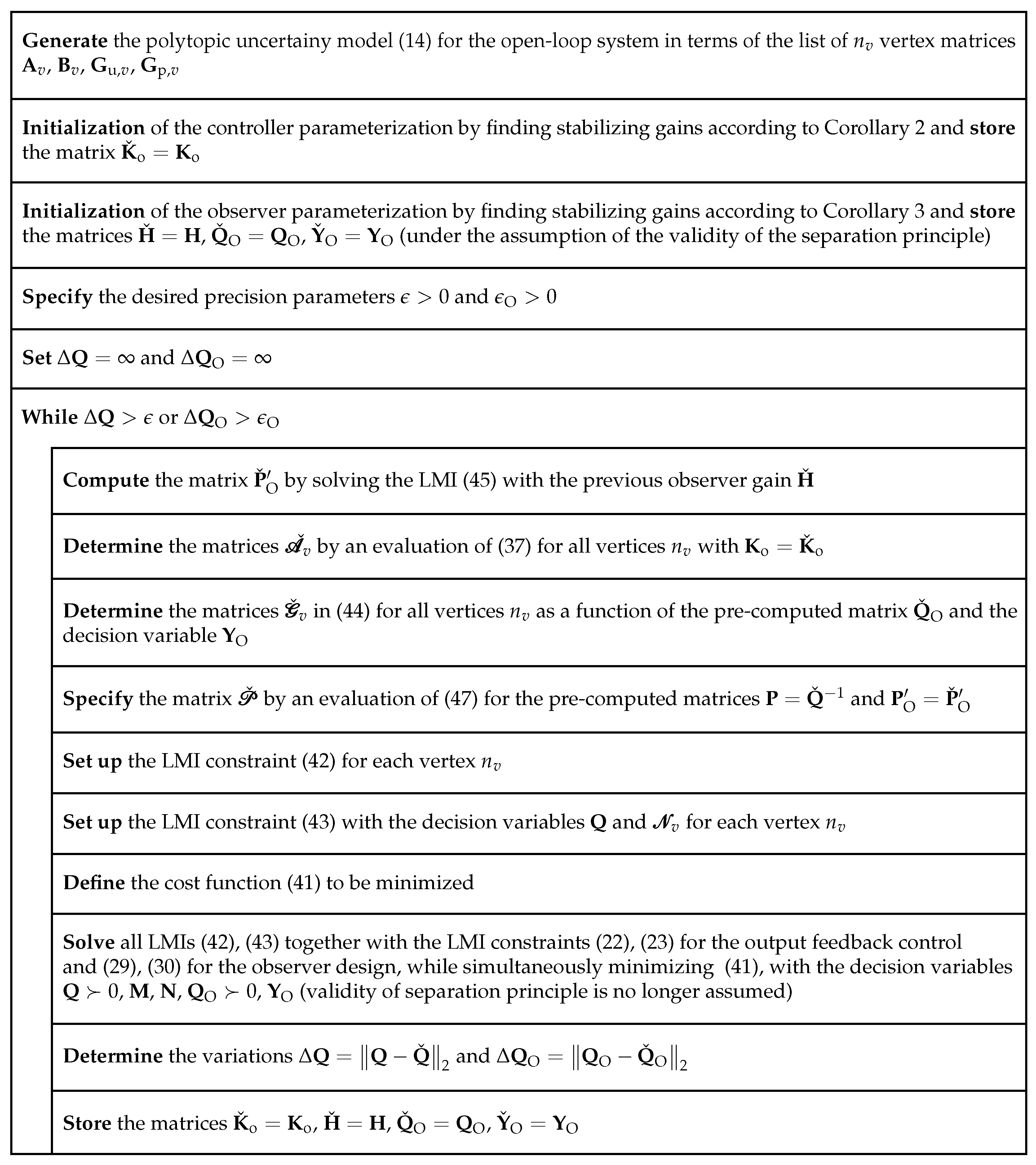
This paper proposes a novel iterative solution that (i) solves the nonlinear matrix inequalities for a combined control and observer design of linear continuous-time processes with polytopic parameter uncertainty in an iterative manner and (ii) generalizes the procedures from [14] to optimize the controller and observer gains so that the sensitivity against actuator, process, and sensor noise on the closed-loop trajectories and the observer’s error dynamics is minimized by means of the simultaneous control and observer design. Besides the design of observer-based full state feedback controllers, our approach is also capable of designing output feedback control laws, where the measured outputs and fed-back quantities do not necessarily have to coincide. Due to the inclusion of the state observer in the design procedure, the proposed approach is more general than the robust output feedback design that was proposed by Gershon and Shaked in [16] for discrete-time systems.

Finally, the work of Do et al. in [17] should be mentioned. There, a combined control and observer design was performed. However, the authors do not aim at directly minimizing the domain for which stability in a stochastic sense cannot be proven. Instead, they aim to achieve the stability of the overall closed-loop control structure by suppressing the influence of disturbances by means of a frequency response shaping approach.

This paper is structured as follows. After a short introductory example in Section 2, Section 3 reviews our results published in [14] to turn them into a novel iterative LMI approach for an optimized, guaranteed stabilizing combined control and observer synthesis in Section 4. The efficiency of this approach is demonstrated in Section 5 in numerical simulations for the stabilization of the Zeeman catastrophe machine [18]. The stabilization is performed along the curve of input-dependent unstable equilibria. In addition, a representative tracking control task is presented, in which the feedforward control signal is determined by a P-type iterative learning control approach [19,20]. Finally, conclusions and an outlook on future work are provided in Section 6.

2. Observer-Based Control of Systems with Polytopic Uncertainty: A Cautionary Tale

As an introductory warning example, consider the unstable linear plant

$$\dot{x}\left(t\right)=a·x\left(t\right)+u\left(t\right)$$

(1)

with the interval parameter $a\in \left[a\right]=\left[a;\overline{a}\right]=\left[1;3\right]$. It is desired to parameterize a linear feedback controller $u\left(t\right)=-k·\widehat{x}\left(t\right)$, where $\widehat{x}\left(t\right)$ is a filtered state estimate resulting from the observer

$$\dot{\widehat{x}}\left(t\right)=a_{\mathrm{nom}}·\widehat{x}\left(t\right)+u\left(t\right)+h·\left(y_{\mathrm{m}}\left(t\right)-\widehat{x}\left(t\right)\right).$$

(2)

Here, $y_{\mathrm{m}}\left(t\right)=x\left(t\right)$ represents the measured plant output and $a_{\mathrm{nom}}$ is a fixed point-valued parameter taken from the interval $\left[a\right]$.

Remark 1.

Because this example should purely visualize the loss of validity of the classical separation principle of control and observer synthesis due to the bounded uncertainty of the parameter $a\in \left[a\right]$, stochastic process and sensor noise are not considered in this section. Noise will be accounted for systematically in Section 3 and Section 4.

A classical control synthesis for the system model (1) would assume that $\widehat{x}\left(t\right)\approx x\left(t\right)$ holds. Then, the closed-loop dynamics result in

$$\dot{x}\left(t\right)=\left(a-k\right)·x\left(t\right),$$

(3)

which become asymptotically stable if the controller gain k is chosen so that

$$k>\overline{a}=3$$

(4)

holds.

Similarly, the observer error dynamics with $e\left(t\right)=x\left(t\right)-\widehat{x}\left(t\right)$ would classically be stated as

$$\dot{e}\left(t\right)=\left(a-h\right)·e\left(t\right),$$

(5)

under the assumption of an identical parameter a in both the plant and observer model, where

$$h>\overline{a}=3$$

(6)

would ensure stability.

When considering that $a_{\mathrm{nom}}$ in the observer differential Equation (2) is some point value taken from the interval $\left[\underset{¯}{a};\overline{a}\right]$, the resulting combined system dynamics turn into

$$\left[\begin{array}{c}\dot{x}\left(t\right)\\ \dot{\widehat{x}}\left(t\right)\end{array}\right]=\left[\begin{array}{cc}a& -k\\ h& a_{\mathrm{nom}}-k-h\end{array}\right]·\left[\begin{array}{c}x\left(t\right)\\ \widehat{x}\left(t\right)\end{array}\right]=\tilde{\mathbf{A}}\left(a,a_{\mathrm{nom}},k,h\right)·\left[\begin{array}{c}x\left(t\right)\\ \widehat{x}\left(t\right),\end{array}\right]$$

(7)

for which the control and observer gains k and h need to be chosen so that all eigenvalues of $\tilde{\mathbf{A}}\left(a,a_{\mathrm{nom}},k,h\right)$ are guaranteed to lie strictly within the open left complex half-plane for all possible realizations of $a\in \left[a\right]$.

Due to the simple structure of the scalar system model with a single uncertain parameter, the optimal choice (with respect to maximizing the admissible domains for the gains k and h) is obvious; it would be $a_{\mathrm{nom}}=\overline{a}=3$. However, in more general settings, such simple statements are typically not possible. At least for systems with a small number of uncertain parameters, as well as controller and observer gains, the choice could be assisted analytically by the parameter space approach from [8].

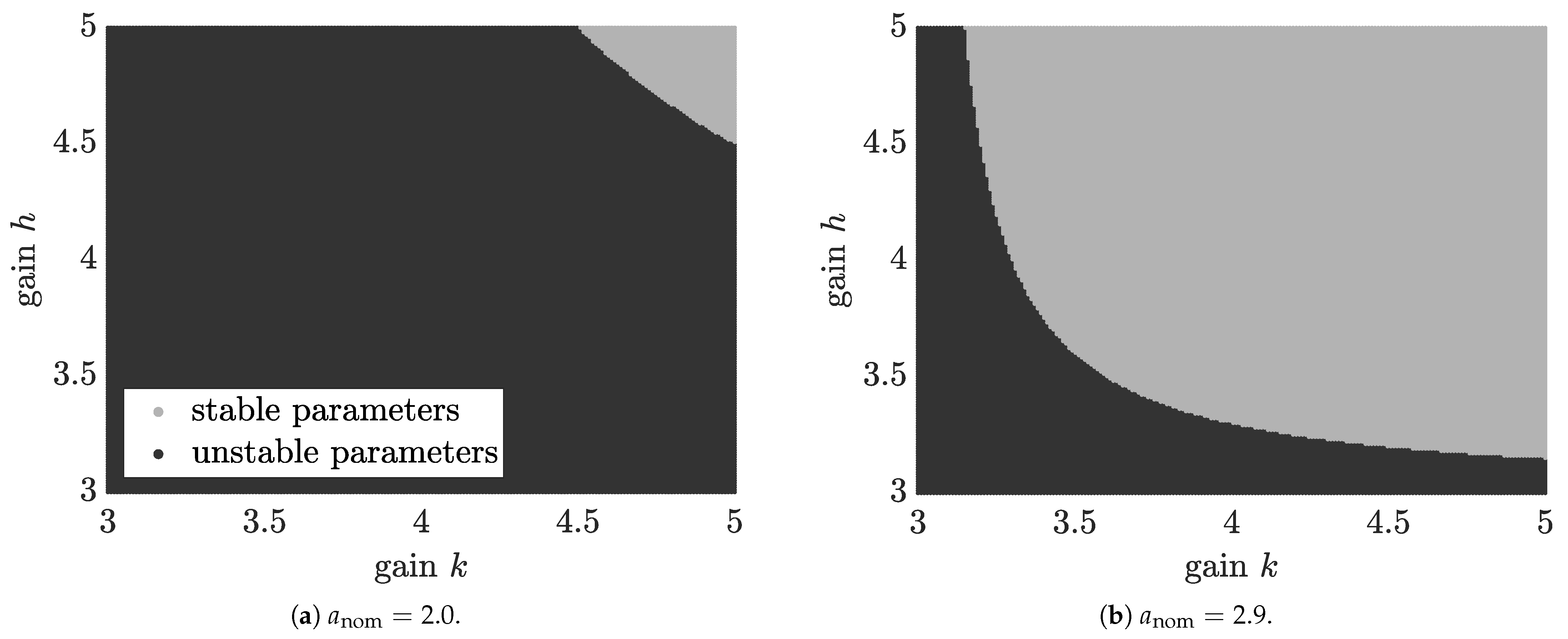
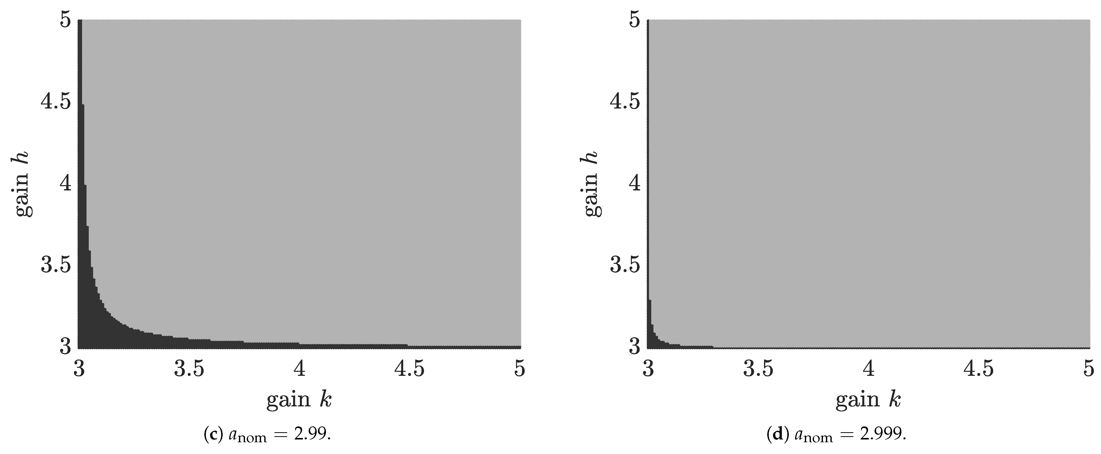
For more complex models, only numerical techniques are helpful for determining the admissible domains of stabilizing controller and observer gains k and h, respectively. For the academic example in this section, a numerical analysis of the stability domains is shown in Figure 1. Domains of robustly stabilizing gains are highlighted in a light gray color, while gains with unstable eigenvalues for at least one $a\in \left[a\right]$ are highlighted in dark gray. Clearly, setting $a_{\mathrm{nom}}$ to a value that is significantly smaller than $\overline{a}$ (e.g., to the interval midpoint $\frac{1}{2}·\left(\underset{¯}{a}+\overline{a}\right)$ in Figure 1a) requires much larger gains for k and h than the settings in Figure 1b–d. The loss of the validity of the separation principle of control and observer design can be seen clearly from the fact that the boundary between stable and unstable realizations is a curved line that is not parallel to the coordinate axes k and h in Figure 1. The separation principle would only hold in cases where the stability boundaries for k and h are fully decoupled.

Figure 1. Stability analysis of the observer-based closed-loop control system (7) for different values of $a_{\mathrm{nom}}$ and $a\in \left[1;3\right]$: The choice of $a_{\mathrm{nom}}\ne \overline{a}$ requires a significant increase of both k and h above the thresholds $k>3$ and $h>3$.

The iterative LMI-based solution procedure given in the following sections provides a systematic approach for stabilizing the observer-based closed-loop control system when the point-valued parameterization of the parallel model in the observer (the parameter $a_{\mathrm{nom}}$ in (Equation (2))) is fixed. In addition to purely finding the stabilizing controller and observer gains, the proposed technique optimizes the gains so that the resulting dynamics become as insensitive as possible against stochastic actuator, process, and sensor noise. An optimization of the point-valued parameters of the parallel model included in the state observer can be considered a subject for future work.

3. Methodological Background: LMI-Based Control and Observer Design

In this paper, dynamic system models are considered, which are given by the stochastic differential equations

$$\mathrm{d}\mathbf{x}\left(t\right)=\mathbf{A}\left(\mathbf{p}\right)·\mathbf{x}\left(t\right)\mathrm{d}t+\mathbf{B}\left(\mathbf{p}\right)·\left(\mathbf{u}\left(t\right)\mathrm{d}t+{\mathbf{G}}_{\mathrm{u}}\left(\mathbf{p}\right)·\mathrm{d}{\mathbf{w}}_{\mathrm{u}}\right)+{\mathbf{G}}_{\mathrm{p}}\left(\mathbf{p}\right)·\mathrm{d}{\mathbf{w}}_{\mathrm{p}}$$

(8)

with the state vector $\mathbf{x}:=\mathbf{x}\left(t\right)\in {\mathbb{R}}^{n_{\mathrm{x}}}$ and the input vector $\mathbf{u}:=\mathbf{u}\left(t\right)\in {\mathbb{R}}^{n_{\mathrm{u}}}$; $\mathbf{A}\left(\mathbf{p}\right)$ and $\mathbf{B}\left(\mathbf{p}\right)$ are the system and input matrices, where $\mathbf{p}\in {\mathbb{R}}^{n_{\mathrm{p}}}$ is a vector of either constant or time-varying bounded parameters. Alternatively, this vector may denote the dependence of all system matrices on the state variables $\mathbf{x}$, cf. [9]. For the sake of a compact notation, all entries of $\mathbf{p}$ are treated as mutually independent with an affine dependence of $\mathbf{A}$ and $\mathbf{B}$ on these quantities. Moreover, ${\mathbf{w}}_{\mathrm{u}}\in {\mathbb{R}}^{m_{\mathrm{u}}}$ and ${\mathbf{w}}_{\mathrm{p}}\in {\mathbb{R}}^{m_{\mathrm{p}}}$ are stochastically independent standard normally distributed Brownian motions of actuator and process noise. In this sense, ${\mathbf{G}}_{\mathrm{u}}\left(\mathbf{p}\right)$ and ${\mathbf{G}}_{\mathrm{p}}\left(\mathbf{p}\right)$ represent the (element-wise non-negative) disturbance input matrices containing the corresponding standard deviations.

The measured system output is given by

$${\mathbf{y}}_{\mathrm{m}}\left(t\right)={\mathbf{C}}_{\mathrm{m}}\mathbf{x}\left(t\right)+{\mathbf{G}}_{\mathrm{m}}{\mathbf{w}}_{\mathrm{m}},$$

(9)

where the output matrix ${\mathbf{C}}_{\mathrm{m}}\in {\mathbb{R}}^{n_{\mathrm{y}}\times n_{\mathrm{x}}}$ is assumed to be exactly known; ${\mathbf{w}}_{\mathrm{m}}$ is the standard normally distributed sensor noise, while ${\mathbf{G}}_{\mathrm{m}}$ is the weighting matrix representing the actual standard deviation of the output disturbance.

In the following, we aim at designing either an observer-based state feedback (Case 1) or an observer-based output feedback control strategy (Case 2). In the second case, the measured output does not necessarily coincide with the system output to be controlled. A linear filter-based output feedback (Case 3), in which the filter is designed in a model-free manner, is only mentioned for the sake of completeness and has been treated by the authors in a separate publication [21]. The reason for this separate investigation is the fact that the design criteria do not fully coincide with the requirements derived for the Cases 1 and 2 in this paper:

Case 1:

The control signal is defined as

$$\mathbf{u}={\mathbf{u}}_{\mathrm{ff}}-\mathbf{K}·\widehat{\mathbf{x}},$$

(10)

where (without loss of generality) ${\mathbf{u}}_{\mathrm{ff}}$ is a constant feedforward signal and $\widehat{\mathbf{x}}$ is the state estimate determined by the robust observer

$$\begin{array}{cc}\hfill \dot{\widehat{\mathbf{x}}}& ={\mathbf{A}}_{\mathrm{nom}}·\widehat{\mathbf{x}}+{\mathbf{B}}_{\mathrm{nom}}·\mathbf{u}+\mathbf{H}·\left({\mathbf{y}}_{\mathrm{m}}-\widehat{\mathbf{y}}\right)\hfill \\ \hfill \widehat{\mathbf{y}}& ={\mathbf{C}}_{\mathrm{m}}·\widehat{\mathbf{x}},\hfill \end{array}$$

(11)

which makes use of the nominal system and input matrices ${\mathbf{A}}_{\mathrm{nom}}$ and ${\mathbf{B}}_{\mathrm{nom}}$, see Section 3.4. For the following stabilization and performance optimization, ${\mathbf{u}}_{\mathrm{ff}}=\mathbf{0}$ is assumed. Desired operating points outside the origin $\mathbf{x}=\mathbf{0}$ are easily achievable by adding suitable nonzero offset terms.

Case 2:

The control signal is defined as

$$\mathbf{u}={\mathbf{u}}_{\mathrm{ff}}-{\mathbf{K}}_{\mathrm{o}}·\mathbf{C}·\widehat{\mathbf{x}},$$

(12)

with the same observer as in (11). Note that the output matrix $\mathbf{C}$ does not necessarily coincide with the matrix ${\mathbf{C}}_{\mathrm{m}}$ defined in (9).

Case 3:

The control signal is defined as

$$\mathbf{u}={\mathbf{u}}_{\mathrm{ff}}-{\mathbf{K}}_{\mathrm{y}}·{\mathbf{C}}_{\mathrm{y}}·{\widehat{\mathbf{y}}}_{\mathrm{f}},$$

(13)

where ${\widehat{\mathbf{y}}}_{\mathrm{f}}$ is a vector consisting of filtered system outputs and estimated output derivatives, cf. [21].

Remark 2.

Case 3 can be interpreted as a dynamic output feedback control approach, whereas the Cases 1 and 2 are model-based approaches employing feedback controllers that rely on an estimation of the complete state vector by an appropriate full observer. It should be noted that the different control structure of Case 3 leads to a similar, however not identical, LMI approach. Therefore, Case 3 is treated separately in [21]. Moreover, as already discussed in [21], Case 3 should typically only be used if a maximum of two time derivatives of measured output signals are estimated with the model-free filter. In all other cases, the observer-based concepts of Cases 1 and 2 are advantageous.

To guarantee solvability of the control design task in all three cases above, it is assumed that the system (8) is stabilizable using either of the system inputs (10), (12), or (13), and that the pair $(\mathbf{A}\left(\mathbf{p}\right),{\mathbf{C}}_{\mathrm{m}})$ is robustly observable (or at least detectable) in Case 1 as well as in Case 2. Here, robust observability is defined as observability of all possible values of the parameters $\mathbf{p}$ according to the definition given in [8]. Note that the requirements of both stabilizability and detectability will not be proven explicitly. These properties are instead verified constructively by determining a solution that ensures input-to-state stability of the system dynamics as well as of the observer’s error dynamics.

3.1. Polytopic Uncertainty Modeling

As shown in [4,6,22], it is possible to describe the influence of uncertainty in many practical applications by bounded uncertainty domains $\mathcal{D}$ of polytope type. There, it is assumed that all system matrices in (8) belong to a convex combination of extremal vertex matrices in the form

$$\begin{array}{cc}\hfill \mathcal{D}=\{& \left[\mathbf{A},\mathbf{B},{\mathbf{G}}_{\mathrm{u}},{\mathbf{G}}_{\mathrm{p}}\right]|\left[\mathbf{A}\left(\xi \right),\mathbf{B}\left(\xi \right),{\mathbf{G}}_{\mathrm{u}}\left(\xi \right),{\mathbf{G}}_{\mathrm{p}}\left(\xi \right)\right]\hfill \\ \hfill & =\sum _{v=1}^{n_v}{\xi }_v·\left[{\mathbf{A}}_v,{\mathbf{B}}_v,{\mathbf{G}}_{\mathrm{u},v},{\mathbf{G}}_{\mathrm{p},v}\right];\sum _{v=1}^{n_v}{\xi }_v=1;{\xi }_v\ge 0\},\hfill \end{array}$$

(14)

where $n_v$ denotes the number of independent extremal realizations for the union of all four matrices included in (14).

3.2. Robust State Feedback Control

In all following subsections, sufficient conditions for asymptotic stability of the closed-loop system dynamics (and the observers’ error dynamics, respectively) are derived on the basis of quadratic, parameter-independent, radially unbounded Lyapunov function candidates

$$V\left(\mathbf{x}\right)=\frac{1}{2}{\mathbf{x}}^T·\mathbf{P}·\mathbf{x}$$

(15)

with the positive definite matrix

$$\mathbf{P}={\mathbf{P}}^T\succ 0$$

(16)

as a free decision variable to be determined during the proposed iterative solution of matrix inequalities.

Theorem 1

([4,6] Sufficient stability condition for full state feedback). Robust asymptotic stability of the closed-loop control system according to Case 1 for a noise- and error-free state feedback (i.e., $\mathbf{x}\equiv \widehat{\mathbf{x}}$) is ensured if the gain matrix $\mathbf{K}$ satisfies the bilinear matrix inequalities

$${\left({\mathbf{A}}_v-{\mathbf{B}}_v\mathbf{K}\right)}^T·\mathbf{P}+\mathbf{P}·\left({\mathbf{A}}_v-{\mathbf{B}}_v\mathbf{K}\right)\prec 0,$$

(17)

$\mathbf{P}={\mathbf{P}}^T\succ 0$, for all polytope vertices $v\in \{1,\dots ,n_v\}$ in (14).

Proof. 

Substituting the control law (10) with ${\mathbf{u}}_{\mathrm{ff}}\equiv \mathbf{0}$ in the deterministic part of the system model (8), computing the time derivative of the Lyapunov function candidate (15), and representing the system matrices $\mathbf{A}\left(\mathbf{p}\right)$ and $\mathbf{B}\left(\mathbf{p}\right)$ by the polytopic uncertainty model (14) leads to

$$\begin{array}{cc}\hfill \dot{V}\left(\mathbf{x}\right)& =\frac{1}{2}{\dot{\mathbf{x}}}^T·\mathbf{P}·\mathbf{x}+\frac{1}{2}{\mathbf{x}}^T·\mathbf{P}·\dot{\mathbf{x}}\hfill \\ \hfill & =\frac{1}{2}{\mathbf{x}}^T·\sum _{v=1}^{n_v}{\xi }_v·\left({\left({\mathbf{A}}_v-{\mathbf{B}}_v\mathbf{K}\right)}^T·\mathbf{P}+\mathbf{P}·\left({\mathbf{A}}_v-{\mathbf{B}}_v\mathbf{K}\right)\right)·\mathbf{x}.\hfill \end{array}$$

(18)

A sufficient stability condition is guaranteed to be satisfied in terms of $\dot{V}\left(\mathbf{x}\right)<0$ for all $\mathbf{x}\ne \mathbf{0}$ if all matrix inequalities (17) hold true for a parameter-independent controller gain $\mathbf{K}$. □

Corollary 1.

To allow for an efficient solution of the bilinear matrix inequalities in Theorem 1 with the help of standard solvers for LMIs such asSeDuMi[23] in combination withYALMIP[24], the linearizing change of variables

$$\mathbf{P}={\mathbf{Q}}^{-1}and\mathbf{K}=\mathbf{Y}\mathbf{P}$$

(19)

is introduced. Multiplying (17) from the left and right with the matrix $\mathbf{Q}$ leads to equivalent LMIs

$${\mathbf{A}}_v\mathbf{Q}+\mathbf{Q}{\mathbf{A}}_v^T-{\mathbf{B}}_v\mathbf{Y}-{\mathbf{Y}}^T{\mathbf{B}}_v^T\prec 0$$

(20)

with $\mathbf{Q}={\mathbf{Q}}^T\succ 0$. Their solution $\mathbf{Q}={\mathbf{P}}^{-1}$ with $\mathbf{Y}=\mathbf{K}{\mathbf{P}}^{-1}$ then needs to be transformed back by means of (19).

3.3. Robust Output Feedback Control

Theorem 2

(Sufficient stability condition for output feedback control). Robust asymptotic stability of the closed-loop control system according to Case 2 for an error-free output feedback (i.e., $\mathbf{C}\mathbf{x}\equiv \mathbf{C}\widehat{\mathbf{x}}$) is ensured if the gain matrix ${\mathbf{K}}_{\mathrm{o}}$ satisfies the bilinear matrix inequalities

$${\left({\mathbf{A}}_v-{\mathbf{B}}_v{\mathbf{K}}_{\mathrm{o}}\mathbf{C}\right)}^T·\mathbf{P}+\mathbf{P}·\left({\mathbf{A}}_v-{\mathbf{B}}_v{\mathbf{K}}_{\mathrm{o}}\mathbf{C}\right)\prec 0,$$

(21)

$\mathbf{P}={\mathbf{P}}^T\succ 0$, for all polytope vertices $v\in \{1,\dots ,n_v\}$ in (14).

Proof. 

The proof of Theorem 2 is a direct consequence of the sufficient stability condition used for the proof of Theorem 1. □

Corollary 2

([25]). For precisely known matrices $\mathbf{C}$, an LMI formulation of Theorem 2 is obtained by introducing a linearizing change of variables with $\mathbf{Q}={\mathbf{P}}^{-1}\succ 0$ and the equality constraints

$$\mathbf{M}\mathbf{C}=\mathbf{C}\mathbf{Q}and\mathbf{N}={\mathbf{K}}_{\mathrm{o}}\mathbf{M}.$$

(22)

Multiplying (21) from the left and right by $\mathbf{Q}$ and considering the relations (22) yields the LMIs

$${\mathbf{A}}_v\mathbf{Q}+\mathbf{Q}{{\mathbf{A}}_v}^T-{\mathbf{B}}_v\mathbf{N}\mathbf{C}-{\mathbf{C}}^T{\mathbf{N}}^T{{\mathbf{B}}_v}^T\prec 0.$$

(23)

If the matrix $\mathbf{C}$, and therefore also $\mathbf{M}$, have full row rank, the resulting controller gain is given by

$${\mathbf{K}}_{\mathrm{o}}=\mathbf{N}{\mathbf{M}}^{-1}.$$

(24)

Remark 3.

In the literature [10,25], an alternative problem formulation is often given in terms of

$$\mathbf{P}{\mathbf{A}}_v+{{\mathbf{A}}_v}^T\mathbf{P}-\mathbf{B}\mathbf{N}\mathbf{C}-{\mathbf{C}}^T{\mathbf{N}}^T{\mathbf{B}}^T\prec 0$$

(25)

with $\mathbf{P}\succ 0$ and the additional equality constraint

$$\mathbf{B}\mathbf{M}=\mathbf{P}\mathbf{B},$$

(26)

leading to ${\mathbf{K}}_{\mathrm{o}}={\mathbf{M}}^{-1}\mathbf{N}$. Applying this formulation is, however, only useful for precisely known matrices $\mathbf{B}$, where $\mathbf{C}$ instead may be subject to a polytopic uncertainty model.

Remark 4.

Theorems 1 and 2 become identical for the case of a full state feedback, namely, for $\mathbf{C}=\mathbf{I}$. Then, the constraint $\mathbf{M}\mathbf{C}=\mathbf{C}\mathbf{Q}$ becomes redundant as $\mathbf{M}=\mathbf{Q}$.

3.4. Robust State Observation

Following the duality principle between control and observer synthesis, as described for example in [10,26], leads to the counterparts of Theorem 1 and Corollary 1 according to the following Theorem 3, where the observer differential equation is given by Equation (11).

Theorem 3

([10] Sufficient stability condition for robust state observer). The error dynamics of a robust state observer according to Equation (11) with the exactly known output matrix ${\mathbf{C}}_{\mathrm{m}}$ are robustly asymptotically stable if the observer gain $\mathbf{H}$ satisfies the bilinear matrix inequalities

$${\left({\mathbf{A}}_v-\mathbf{H}{\mathbf{C}}_{\mathrm{m}}\right)}^T·{\mathbf{P}}_{\mathrm{O}}^{\prime }+{\mathbf{P}}_{\mathrm{O}}^{\prime }·\left({\mathbf{A}}_v-\mathbf{H}{\mathbf{C}}_{\mathrm{m}}\right)\prec 0$$

(27)

for some positive definite matrix ${\mathbf{P}}_{\mathrm{O}}^{\prime }={{\mathbf{P}}_{\mathrm{O}}^{\prime }}^T\succ 0$ at all polytope vertices $v\in \{1,\dots ,n_v\}$ in (14).

As stated before, the matrix ${\mathbf{C}}_{\mathrm{m}}$ in (27) does not necessarily have to be identical to the matrix $\mathbf{C}$ to be fed back in the control law (12). Note that the prime symbol ${\left(·\right)}^{\prime }$ in (27) has been introduced to indicate that the matrix ${\mathbf{P}}_{\mathrm{O}}^{\prime }$ is typically not the same as ${\mathbf{P}}_{\mathrm{O}}$ in the following corollary.

Corollary 3

([10]). To allow for an efficient solution of the bilinear matrix inequalities in Theorem 3, after considering the duality between control and observer synthesis by evaluating the transposed of (27) according to

$$\left({\mathbf{A}}_v-\mathbf{H}{\mathbf{C}}_{\mathrm{m}}\right)·{\mathbf{P}}_{\mathrm{O}}+{\mathbf{P}}_{\mathrm{O}}·{\left({\mathbf{A}}_v-\mathbf{H}{\mathbf{C}}_{\mathrm{m}}\right)}^T\prec 0,$$

(28)

the linearizing change of variables

$${\mathbf{P}}_{\mathrm{O}}={{\mathbf{Q}}_{\mathrm{O}}}^{-1}and\mathbf{H}={\left({\mathbf{Y}}_{\mathrm{O}}{\mathbf{P}}_{\mathrm{O}}\right)}^T$$

(29)

is introduced. Multiplying (27) from the left and right with the matrix ${\mathbf{Q}}_{\mathrm{O}}$ leads to equivalent LMIs

$${\mathbf{A}}_v^T{\mathbf{Q}}_{\mathrm{O}}+{\mathbf{Q}}_{\mathrm{O}}{\mathbf{A}}_v-{\mathbf{C}}_{\mathrm{m}}^T{\mathbf{Y}}_{\mathrm{O}}-{\mathbf{Y}}_{\mathrm{O}}^T{\mathbf{C}}_{\mathrm{m}}\prec 0$$

(30)

for all polytope vertices $v\in \{1,\dots ,n_v\}$ in (14).

4. Main Results: Iterative LMI Solution for a Combined Control and Observer Synthesis in the Presence of Stochastic Noise

This section provides the main result of this paper. It consists of the description of an augmented stochastic differential equation model, comprising the controlled plant as well as the robust state observer. Based on this augmented model, optimality conditions for the combined computation of the control and observer gains are presented which allow us to minimize the size of the domain around the desired operating point for which stability cannot be proven due to the presence of stochastic actuator, process, and sensor noise. For a visualization of such domains in the frame of oscillation attenuation for boom cranes in marine applications, the reader is referred to [27].

4.1. Observer-Based Feedback Control in the Presence of Noise

To ensure stability of the control laws (10) or (12) despite the general invalidity of the separation principle according to Section 2 and to simultaneously optimize the controller and observer gain matrices in Cases 1 and 2, the closed-loop control systems’ dynamics as well as the point-valued observers’ error dynamics ${\mathbf{e}}_v={\mathbf{x}}_v-{\widehat{\mathbf{x}}}_v$ are described by using a combined set of stochastic differential equation models. In the following, all system models are derived for each of the worst-case realizations $v\in \{1,\dots ,n_v\}$, to simultaneously account for bounded parameter uncertainty and stochastic noise.

For that purpose, the deterministic system models from the previous section (i.e., the noise-free, however, parameter-dependent terms) are extended by the terms for stochastic process and sensor noise as well as by accounting for the control signals

$$\begin{array}{cc}\hfill {\mathbf{u}}_v=-{\mathbf{K}}_{\mathrm{o}}\mathbf{C}{\widehat{\mathbf{x}}}_v& =-{\mathbf{K}}_{\mathrm{o}}\mathbf{C}·\left({\mathbf{x}}_v-{\mathbf{e}}_v\right).\hfill \end{array}$$

(31)

Hence, each vertex realization for the closed-loop control system is represented by a stochastic differential equation

$$\begin{array}{cc}\hfill \mathrm{d}{\mathbf{x}}_v& =\left(\left({\mathbf{A}}_v-{\mathbf{B}}_v{\mathbf{K}}_{\mathrm{o}}\mathbf{C}\right){\mathbf{x}}_v+{\mathbf{B}}_v{\mathbf{K}}_{\mathrm{o}}\mathbf{C}{\mathbf{e}}_v\right)\mathrm{d}t+\left[\begin{array}{cc}{\mathbf{B}}_v{\mathbf{G}}_{\mathrm{u},v}& {\mathbf{G}}_{\mathrm{p},v}\end{array}\right]·\left[\begin{array}{c}\mathrm{d}{\mathbf{w}}_{\mathrm{u}}\\ \mathrm{d}{\mathbf{w}}_{\mathrm{p}}\end{array}\right].\hfill \end{array}$$

(32)

Here and in the following, $\mathbf{C}\equiv \mathbf{I}$ and ${\mathbf{K}}_{\mathrm{o}}\equiv \mathbf{K}$ hold for Case 1.

Similarly, the stochastic differential equation for the observer dynamics at each vertex v is obtained as

$$\mathrm{d}{\widehat{\mathbf{x}}}_v=\left(\left({\mathbf{A}}_{\mathrm{nom}}-{\mathbf{B}}_{\mathrm{nom}}{\mathbf{K}}_{\mathrm{o}}\mathbf{C}\right){\widehat{\mathbf{x}}}_v+\mathbf{H}{\mathbf{C}}_{\mathrm{m}}{\mathbf{e}}_v\right)\mathrm{d}t+\mathbf{H}{\mathbf{G}}_{\mathrm{m}}\mathrm{d}{\mathbf{w}}_{\mathrm{m}}.$$

(33)

The latter leads to the associated error dynamics

$$\begin{array}{cc}\hfill \mathrm{d}{\mathbf{e}}_v& =\left(\left(\left({\mathbf{A}}_v-{\mathbf{A}}_{\mathrm{nom}}\right)-\left({\mathbf{B}}_v-{\mathbf{B}}_{\mathrm{nom}}\right){\mathbf{K}}_{\mathrm{o}}\mathbf{C}\right){\mathbf{x}}_v\right)\mathrm{d}t\hfill \\ \hfill & \phantom{=}+\left(\left(\left({\mathbf{A}}_{\mathrm{nom}}-\mathbf{H}{\mathbf{C}}_{\mathrm{m}}\right)-\left({\mathbf{B}}_{\mathrm{nom}}-{\mathbf{B}}_v\right){\mathbf{K}}_{\mathrm{o}}\mathbf{C}\right){\mathbf{e}}_v\right)\mathrm{d}t\hfill \\ \hfill & \phantom{=}+\left[\begin{array}{ccc}{\mathbf{B}}_v{\mathbf{G}}_{\mathrm{u},v}& {\mathbf{G}}_{\mathrm{p},v}& -\mathbf{H}{\mathbf{G}}_{\mathrm{m}}\end{array}\right]·\left[\begin{array}{c}\mathrm{d}{\mathbf{w}}_{\mathrm{u}}\\ \mathrm{d}{\mathbf{w}}_{\mathrm{p}}\\ \mathrm{d}{\mathbf{w}}_{\mathrm{m}}\end{array}\right].\hfill \end{array}$$

(34)

As discussed in [14], it may be impossible to verify stability in the close vicinity of the desired stationary operating point in the presence of stochastic noise. This is true even if a robust stabilization by simultaneously designing the controller and observer for the noise-free polytopic uncertainty model is successful.

To design a state observer minimizing the sensitivity against noise, our previous work [14] suggests estimating the volume of an ellipsoid centered at the desired operating point for which stability properties cannot be proven. For the case of exactly known system models, an LMI-based optimization approach was introduced in [14] to reduce the corresponding ellipsoid volume. This approach is now extended by the following two aspects: (i) simultaneously computing the controller and observer gains in a jointly stabilizing sense in the presence of noise, as well as (ii) additionally considering the goal of achieving insensitivity against bounded parameter uncertainty in the system matrices by the minimization of the aforementioned ellipsoid volume.

For that purpose, define an augmented vector

$${\mathbf{z}}_v={\left[\begin{array}{cc}{\mathbf{x}}_v^T& {\mathbf{e}}_v^T\end{array}\right]}^T$$

(35)

consisting of system states and estimation errors for each extremal system representation from the polytope (14). The corresponding stochastic differential equations are given by

$$\mathrm{d}{\mathbf{z}}_v={\mathcal{A}}_v·{\mathbf{z}}_v\mathrm{d}t+{\mathcal{G}}_v·\left[\begin{array}{c}\mathrm{d}{\mathbf{w}}_{\mathrm{u}}\\ \mathrm{d}{\mathbf{w}}_{\mathrm{p}}\\ \mathrm{d}{\mathbf{w}}_{\mathrm{m}}\end{array}\right]$$

(36)

with

$${\mathcal{A}}_v=\left[\begin{array}{cc}{\mathbf{A}}_v-{\mathbf{B}}_v{\mathbf{K}}_{\mathrm{o}}\mathbf{C}& {\mathbf{B}}_v{\mathbf{K}}_{\mathrm{o}}\mathbf{C}\\ {\mathcal{A}}_{2,1,v}& {\mathcal{A}}_{2,2,v}\end{array}\right],$$

(37)

where the sub-matrices in the second row result in

$${\mathcal{A}}_{2,1,v}=\left({\mathbf{A}}_v-{\mathbf{A}}_{\mathrm{nom}}\right)-\left({\mathbf{B}}_v-{\mathbf{B}}_{\mathrm{nom}}\right){\mathbf{K}}_{\mathrm{o}}\mathbf{C}$$

(38)

and

$${\mathcal{A}}_{2,2,v}=\left({\mathbf{A}}_{\mathrm{nom}}-\mathbf{H}{\mathbf{C}}_{\mathrm{m}}\right)-\left({\mathbf{B}}_{\mathrm{nom}}-{\mathbf{B}}_v\right){\mathbf{K}}_{\mathrm{o}}\mathbf{C}.$$

(39)

Similarly, the augmented matrix of noise standard deviations turns into

$${\mathcal{G}}_v=\left[\begin{array}{ccc}{\mathbf{B}}_v{\mathbf{G}}_{\mathrm{u},v}& {\mathbf{G}}_{\mathrm{p},v}& \mathbf{0}\\ {\mathbf{B}}_v{\mathbf{G}}_{\mathrm{u},v}& {\mathbf{G}}_{\mathrm{p},v}& -\mathbf{H}{\mathbf{G}}_{\mathrm{m}}\end{array}\right].$$

(40)

Note that for the simplified case of [14] without parameter uncertainty, the sub-matrices in (38) and (39) turn into ${\mathcal{A}}_{2,1,v}=\mathbf{0}$ and ${\mathcal{A}}_{2,2,v}={\mathbf{A}}_{\mathrm{nom}}-\mathbf{H}{\mathbf{C}}_{\mathrm{m}}$ with ${\mathbf{A}}_{\mathrm{nom}}\equiv {\mathbf{A}}_v$ and ${\mathbf{B}}_{\mathrm{nom}}\equiv {\mathbf{B}}_v$. For this case, the separation principle holds and the observer and controller parameterization (hence also their optimization) can be performed independently.

The following subsection introduces a cost function J that can be minimized in an iterative manner by applying state-of-the-art LMI solvers, such as SeDuMi [23] in combination with YALMIP [24]. Thereby, the controller and observer gains, as well as the Lyapunov function candidate, are computed in parallel.

4.2. Optimality of the Noise Insensitive Observer-Based Control Design

Theorem 4

(Optimal control and observer parameterization). The parameterization of the observer-based controller for the augmented system (36)–(40) is optimal in the sense of a minimization of the influence of noise if the controller and observer gains are chosen to minimize the cost function

$$J=\sum _{v=1}^{n_v}\left(\frac{\mathrm{trace}\left\{{\mathcal{N}}_v\right\}}{det\left(-{\check{\overline{\mathcal{A}}}}_v\right)}·\frac{det\left({\check{\mathbf{P}}}_{\mathrm{O}}^{\prime }\right)}{det\left(\check{\mathbf{Q}}\right)}\right)$$

(41)

with ${\mathcal{N}}_v={\mathcal{N}}_v^T\succ 0$ and

$${\check{\overline{\mathcal{A}}}}_v:={\check{\mathcal{A}}}_v^T\check{\mathcal{P}}+\check{\mathcal{P}}{\check{\mathcal{A}}}_v\prec 0,$$

(42)

where

$$\left[\begin{array}{cc}{\mathcal{N}}_v& {\check{\mathcal{G}}}_v^T\\ {\check{\mathcal{G}}}_v& \left[\begin{array}{cc}\mathbf{Q}& \mathbf{0}\\ \mathbf{0}& {\left({\check{\mathbf{P}}}_{\mathrm{O}}^{\prime }\right)}^{-1}\end{array}\right]\end{array}\right]\succ 0,$$

(43)

$${\check{\mathcal{G}}}_v=\left[\begin{array}{ccc}{\mathbf{B}}_v{\mathbf{G}}_{\mathrm{u},v}& {\mathbf{G}}_{\mathrm{p},v}& \mathbf{0}\\ {\mathbf{B}}_v{\mathbf{G}}_{\mathrm{u},v}& {\mathbf{G}}_{\mathrm{p},v}& -{\check{\mathbf{Q}}}_{\mathrm{O}}^{-1}{\mathbf{Y}}_{\mathrm{O}}^T{\mathbf{G}}_{\mathrm{m}}\end{array}\right],$$

(44)

and

$${\left({\mathbf{A}}_v-\check{\mathbf{H}}{\mathbf{C}}_{\mathrm{m}}\right)}^T·{\check{\mathbf{P}}}_{\mathrm{O}}^{\prime }+{\check{\mathbf{P}}}_{\mathrm{O}}^{\prime }·\left({\mathbf{A}}_v-\check{\mathbf{H}}{\mathbf{C}}_{\mathrm{m}}\right)\prec 0$$

(45)

with $\check{\mathbf{H}}={\check{\mathbf{Q}}}_{\mathrm{O}}^{-1}{{\check{\mathbf{Y}}}_{\mathrm{O}}}^T$ hold. Here, $\check{\left(·\right)}$ symbols indicate an iterative evaluation, where all such values are replaced by the outcome of the previous iteration stage, especially by inserting the previous gain values into (37) to obtain the matrices ${\check{\mathcal{A}}}_v$ in (42).

Proof. 

Define a quadratic form

$$V\left({\mathbf{z}}_v\right)=\frac{1}{2}{\mathbf{z}}_v^T·\mathcal{P}·{\mathbf{z}}_v$$

(46)

as the candidate for a Lyapunov function with the block diagonal matrix

$$\mathcal{P}=\mathrm{blkdiag}\left(\mathbf{P},{\mathbf{P}}_{\mathrm{O}}^{\prime }\right)=\left[\begin{array}{cc}\mathbf{P}& \mathbf{0}\\ \mathbf{0}& {\mathbf{P}}_{\mathrm{O}}^{\prime }\end{array}\right]$$

(47)

consisting of those matrices that were obtained from the Corollaries 1 or 2, as well as from Theorem 3.

The corresponding time derivative of (46) is computed by applying the Itô differential operator [14,15]. It leads to the expression

$$\begin{array}{cc}\hfill L\left(V\right)& =\frac{1}{2}\left({\mathbf{z}}_v^T\left({\mathcal{A}}_v^T\mathcal{P}+\mathcal{P}{\mathcal{A}}_v\right){\mathbf{z}}_v+\mathrm{trace}\left\{{\mathcal{G}}_v^T\mathcal{P}{\mathcal{G}}_v\right\}\right).\hfill \end{array}$$

(48)

Despite the strict negative definiteness of ${\mathcal{A}}_v^T\mathcal{P}+\mathcal{P}{\mathcal{A}}_v$ (corresponding to the asymptotic stability of the deterministic part of the augmented system model due to the existence of a positive definite matrix $\mathcal{P}={\mathcal{P}}^T\succ 0$), the value of $L\left(V\right)$ may become positive in the close vicinity of ${\mathbf{z}}_v=\mathbf{0}$ due to persistent stochastic excitation. The non-provable stability domain is, hence, characterized by the interior of an ellipsoid that is described by the boundary $L\left(V\right)=0$ according to

$${\mathbf{z}}_v^T{\mathcal{M}}_v^{-1}{\mathbf{z}}_v-1=0,$$

(49)

where

$${\mathcal{M}}_v^{-1}=\left(\frac{-{\overline{\mathcal{A}}}_v}{\mathrm{trace}\left\{{\mathcal{G}}_v^T\mathcal{P}{\mathcal{G}}_v\right\}}\right)$$

(50)

and

$${\overline{\mathcal{A}}}_v:={\mathcal{A}}_v^T\mathcal{P}+\mathcal{P}{\mathcal{A}}_v\prec 0.$$

(51)

The volume of this ellipsoid is proportional to

$$\sqrt{det\left({\mathcal{M}}_v\right)}=\sqrt{\frac{\mathrm{trace}\left\{{\mathcal{G}}_v^T\mathcal{P}{\mathcal{G}}_v\right\}}{det\left(-{\overline{\mathcal{A}}}_v\right)}}.$$

(52)

Following the same steps as in ([14], Equations (17)–(20)), it is desired to minimize the quality criterion

$${\mathcal{J}}_v=\frac{\mathrm{trace}\left\{{\mathcal{G}}_v^T\mathcal{P}{\mathcal{G}}_v\right\}}{det\left(-{\overline{\mathcal{A}}}_v\right)}·\frac{det\left({\mathbf{P}}_{\mathrm{O}}^{\prime }\right)}{det\left(\mathbf{Q}\right)}$$

(53)

by tuning the control and observer gains, where the second factor helps to maximize the domains for which the linear feedback in the closed-loop system is bounded by some positive constant [28].

According to [28], multiplicative couplings between $\mathcal{P}$ and the gains included in ${\mathcal{G}}_v$ are removed by an iterative LMI formulation of the optimization task. For that purpose, the term ${\mathcal{G}}_v^T\mathcal{P}{\mathcal{G}}_v$ is relaxed into the matrix inequality

$${\mathcal{N}}_v\succ {\mathcal{G}}_v^T\mathcal{P}{\mathcal{G}}_v\mathrm{corresponding}\mathrm{to}{\mathcal{N}}_v-{\mathcal{G}}_v^T\mathcal{P}{\mathcal{G}}_v\succ 0$$

(54)

with ${\mathcal{N}}_v={\mathcal{N}}_v^T\succ 0$. The inequality (54) is finally re-written by applying the Schur complement formula according to

$$\left[\begin{array}{cc}{\mathcal{N}}_v& {\mathcal{G}}_v^T\\ {\mathcal{G}}_v& \left[\begin{array}{cc}\mathbf{Q}& \mathbf{0}\\ \mathbf{0}& {\left({\mathbf{P}}_{\mathrm{O}}^{\prime }\right)}^{-1}\end{array}\right]\end{array}\right]\succ 0.$$

(55)

The proof is completed by approximating ${\left({\mathbf{P}}_{\mathrm{O}}^{\prime }\right)}^{-1}$ with the solution of the inequality (45) and by replacing all nonlinearities related to the gains and parameterizations of $V\left({\mathbf{z}}_v\right)$ in (46) by the results of the preceding iteration step. □

Remark 5.

The pure block diagonal structure of this matrix $\mathcal{P}$ in (47) with independent parameters for the state and error dynamics, may introduce some degree of conservativeness. However, the positive definiteness of this matrix always guarantees closed-loop stability (see the discussion of Equation (48)). Moreover, the simulations in the following section have shown that the resulting control signals outperform classical design approaches in terms of a reduction of the control effort. In addition, notice that the obtained solution can be conservative due to the use of a common quadratic Lyapunov function for the whole polytope. The use of parameter-dependent Lyapunov functions, such as those discussed in [29] for discrete-time processes with time-varying parameters, will be a subject of future research.

4.3. Summary of the Proposed Algorithm and Further Discussion

The proposed iterative LMI formulation of the combined optimization of control and observer gains for linear systems with polytopic parameter uncertainty and stochastic process, actuator, and sensor noise is summarized in the structure diagram in Figure 2.

Figure 2. Structure diagram of the proposed offline control and observer parameterization.

For the application scenario considered in the following section, the proposed iterative solution technique converged to constant control and observer gains in less than 20 iterations. It should be pointed out that each control and observer parameterization—for which all augmented system matrices (37) can be proven to be asymptotically stable with the help of a common Lyapunov function candidate—stabilizes the deterministic part of the closed-loop control structure with certainty. Hence, a comparison of the optimized cost function value according to (41), after convergence of the iterative optimization procedure and the result of an evaluation of this cost function for a non-optimized, although guaranteed stabilizing parameterization, may be interpreted as the achieved enhancement of robustness. In general, this cost function value is proportional to the average size of the domain of non-provable contractivity around a desired operating point due to noise, where ${\mathcal{J}}_v$ is evaluated for each of the vertices of the polytopic uncertainty representation.

5. Simulation Results

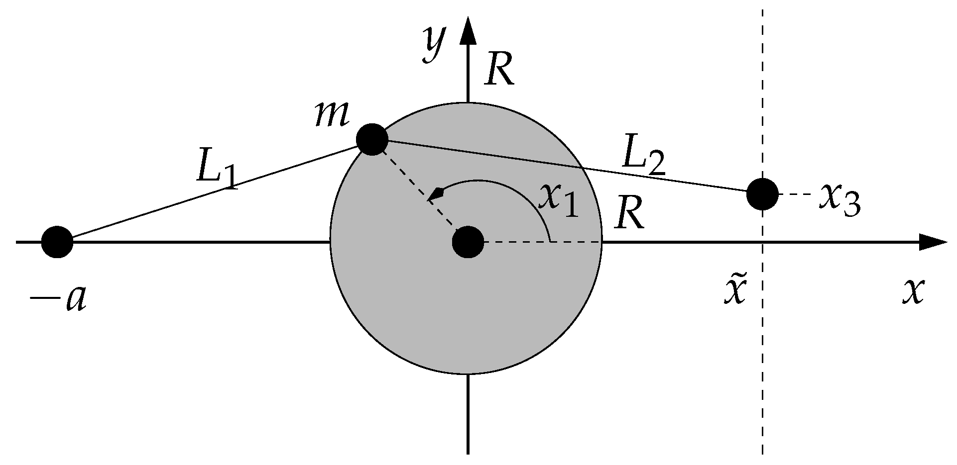
As a benchmark for the proposed control design, we consider the Zeeman catastrophe machine illustrated in Figure 3. It consists of a disc of radius R that can rotate freely around its center at the origin of the $(x,y)$-plane. The angle of orientation $x_1$ (with corresponding velocity $x_2$) can be manipulated by using the position $x_3$ as a control input. This position is assumed to be controlled by an actuator with a non-negligible time constant T, where u denotes the control signal in terms of the desired value for $x_3$.

Figure 3. Application scenario: Zeeman catastrophe machine.

5.1. Modeling

Depending on the location $\tilde{x}$, which is assumed to be fixed, this simple mechanical setup with the connecting elements of the variable lengths $L_1$ and $L_2$, which are given by linear springs with stiffness k, can show nonlinear behavior including hysteresis and chaotic motion [18]. Both springs have the nominal length $L_0$.

The first goal of designing a partial state feedback controller (using only the measurable angle $x_1$ and its derivative $x_2$, where both are smoothened and estimated by a state observer) is to realize a stable transition between two bifurcation points at which the open-loop dynamics change between asymptotic stability and instability (represented by a jump-like motion between two significantly different angles). Second, a tracking controller is designed, which allows for following a reference trajectory $y_{\mathrm{d}}$ for the angle $x_1$.

According to the discussion above, the controller is parameterized with the output matrix

$$\mathbf{C}=\left[\begin{array}{ccc}1& 0& 0\\ 0& 1& 0\end{array}\right],$$

(56)

while

$${\mathbf{C}}_{\mathrm{m}}=\left[\begin{array}{ccc}1& 0& 0\end{array}\right]$$

(57)

represents the sensor’s relation to the state vector.

The equations of motion of this system

$$\begin{array}{cc}\hfill {\dot{x}}_1& =x_2\hfill \\ \hfill {\dot{x}}_2& =\frac{k}{mR}·\left(\frac{L_1-L_0}{L_1}a-\frac{L_2-L_0}{L_2}\tilde{x}\right)sin\left(x_1\right)-d{x}_2+\frac{k}{mR}·\frac{L_2-L_0}{L_2}·cos\left(x_1\right)·x_3\hfill \\ \hfill {\dot{x}}_3& =\frac{1}{T}·\left(-x_3+u\right)\hfill \end{array}$$

(58)

with the velocity–proportional damping term $d{x}_2$ and the state-dependent spring lengths

$$\begin{array}{cc}\hfill L_1& =\sqrt{{\left(Rcos\left(x_1\right)+a\right)}^2+\left(Rsin{\left(x_1\right)}^2\right)}\hfill \end{array}$$

(59)

and

$$\begin{array}{cc}\hfill 1-1L_2& =\sqrt{{\left(\tilde{x}-Rcos\left(x_1\right)\right)}^2+\left(x_3-Rsin{\left(x_1\right)}^2\right)}\hfill \end{array}$$

(60)

can be derived on the basis of Lagrange’s equations of second kind. For this derivation, it is assumed that the total mass m of the system is located at a single point on the edge of the rotating disc.

For the LMI-based design procedure, the system model is re-written into the quasi-linear form

$$\dot{\mathbf{x}}=\left[\begin{array}{ccc}0& 1& 0\\ a_{21}& -d& a_{23}\\ 0& 0& -\frac{1}{T}\end{array}\right]·\mathbf{x}+\left[\begin{array}{c}0\\ 0\\ \frac{1}{T}\end{array}\right]·u$$

(61)

of a polytopic uncertainty system model with ${\mathbf{A}}_v$ and $n_v=4$, where

$$a_{21}=\frac{k}{mR}·\left(\frac{L_1-L_0}{L_1}a-\frac{L_2-L_0}{L_2}\tilde{x}\right)\frac{sin\left(x_1\right)}{x_1}\in \left[-5.2;14.4\right]$$

(62)

and

$$a_{23}=\frac{k}{mR}·\frac{L_2-L_0}{L_2}·cos\left(x_1\right)\in \left[-256;-17\right].$$

(63)

These intervals have been determined for the parameters $T=0.05$, $k=5$, $m=0.1$, $R=0.15$, $L_0=0.1$, $a=0.3$, $\tilde{x}=0.23$, $d=0.5$ and the worst-case operating domains

$$x_1\in \left[-265;-95\right]·\frac{\pi }{180}$$

(64)

and

$$x_3\in \left[-0.2;0.2\right].$$

(65)

All of these parameters and state variables are assumed to be given in terms of corresponding SI units.

Remark 6.

In the following simulations, the nonlinear model is used to represent the controlled plant and observer. The observer gain $\mathbf{H}$ is designed according to Section 4 with a point-valued system matrix ${\mathbf{A}}_{\mathrm{nom}}$ given by the nominal values of the quasi-linear form. Note that this is only one solution of the parameter-dependent observer matrix $\mathbf{A}\left(\xi \right)$. This simplification is possible under the assumption that both tracking and state estimation errors are small. In general, however, the stability of the nonlinear observer can be proven by checking the stability of all ${\left(2n_{\mathrm{x}}\right)}^2$ combinations of the vertex matrices ${\mathbf{A}}_v$ of the controlled plant to each extremal system matrix ${\mathbf{A}}_v$ of the observer.

5.2. Tracking the Unstable Branch of the Bifurcation Diagram

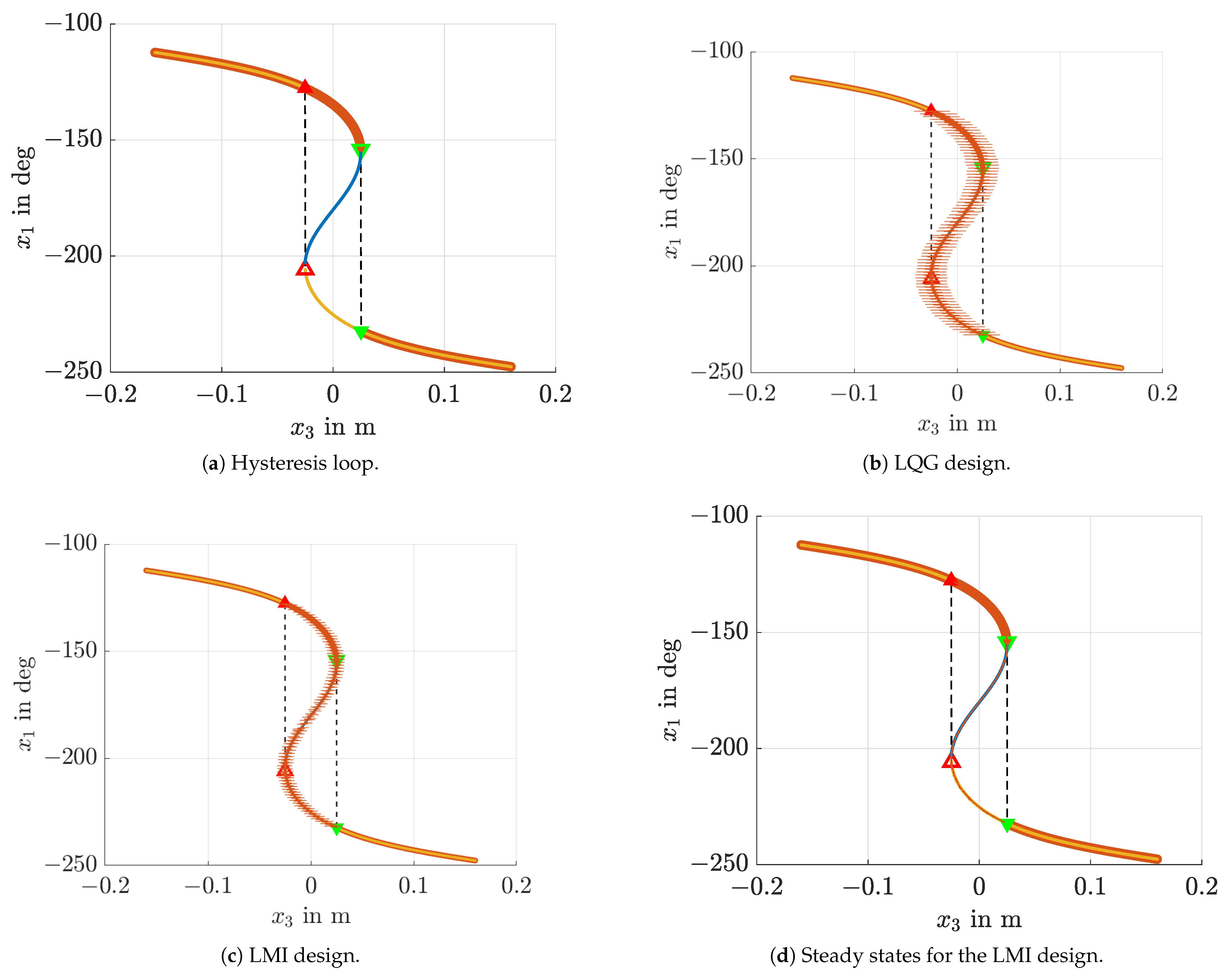
Figure 4a shows the numerically computed equilibria of the system (58) in dependence of piecewise constant inputs $u=x_3$. The hysteresis behavior of the open-loop system can be clearly seen so that starting with angles of approximately $-{110}^{\circ }$, an increase of $x_3$ leads to a jump in the angle $x_1$ (transition from the open to the filled green triangle at some $x_3>0$ in Figure 4), while successively reducing $x_3$ leads to a jump between two different angles for some $x_3<0$ (red triangles in Figure 4). Figure 4a can be interpreted as a bifurcation diagram in the phase space, where the branch between both open green and red triangles is unstable and is not visible in an open-loop operation of the system.

Figure 4. Guidance of the Zeeman catastrophe machine along the unstable branch of equilibria in the $(x_3,x_1)$-plane; comparison of an observer-based full state feedback control parameterized by the LQG technique with the LMI-based parameterization of (12).

However, this branch can be visualized by using the closed-loop control strategy as shown in Figure 4b,c with

$$u=-k_1·\left(x_1-y_{\mathrm{d}}\right)-k_2{x}_2-k_3{x}_3,$$

(66)

where $y_{\mathrm{d}}$ is a piecewise constant reference signal and $k_3=0$ holds in the second scenario due to the choice of $\mathbf{C}$ according to (56) for the LMI-based controller (12).

For the sake of comparison with a standard approach (which, however, does not strictly guarantee closed-loop stability due to the parameter dependency of the system model), an LQG approach has been implemented additionally. It makes use of a continuous-time steady-state Extended Kalman Filter. Both LQG and LMI approaches are parameterized with ${\mathbf{G}}_{\mathrm{p}}={10}^{-2}·\mathbf{I}$, $g_{\mathrm{u}}=0$, and $g_{\mathrm{m}}={10}^{-2}$ in this subsection, where ${\mathbf{C}}_{\mathrm{m}}$ is chosen according to (57).

The controller optimization in the LQG case was performed with $\mathbf{Q}=\mathbf{I}$ and $R=1$ for the point-valued parameters $a_{21}=14.4$ and $a_{23}=-17$. These values were chosen to reflect the strongest instability of the open-loop plant for the control synthesis. Due to the state dependency of the system matrix in (61), this parameterization does not provide a strict proof of stability. In contrast, the LMI approach provides a strict proof of stability and considerably reduced deviations in transient operation from the unstable branch of the bifurcation diagram compared to the LQG design. To limit the observer’s eigenvalues so that a simulation with a fixed step size of ${10}^{-3}$ is admissible, the heuristically chosen penalty term $5·{10}^{-5}·{\parallel {\mathbf{Y}}_{\mathrm{O}}\parallel }_2$ was added onto J, defined in (41).

All simulations were performed for piecewise constant signals for $y_{\mathrm{d}}$ (hold time of $5\mathrm{s}$) with increments of approximately $1.{41}^{\circ }$. If only the terminal states of each step are plotted (cf. Figure 4d), the LMI-case reconstructs the exact unstable branch with deviations of less than ${10}^{-4}$, which is slightly better than in the LQG case. Obviously, the LMI-based solution approach does not only provide a strict proof of stability of the observer-based control structure but in addition, it leads to a significant reduction of the control effort, resulting also in much smoother values for $x_3$ in Figure 4c. The reduction of the control effort is investigated in more detail in the following example.

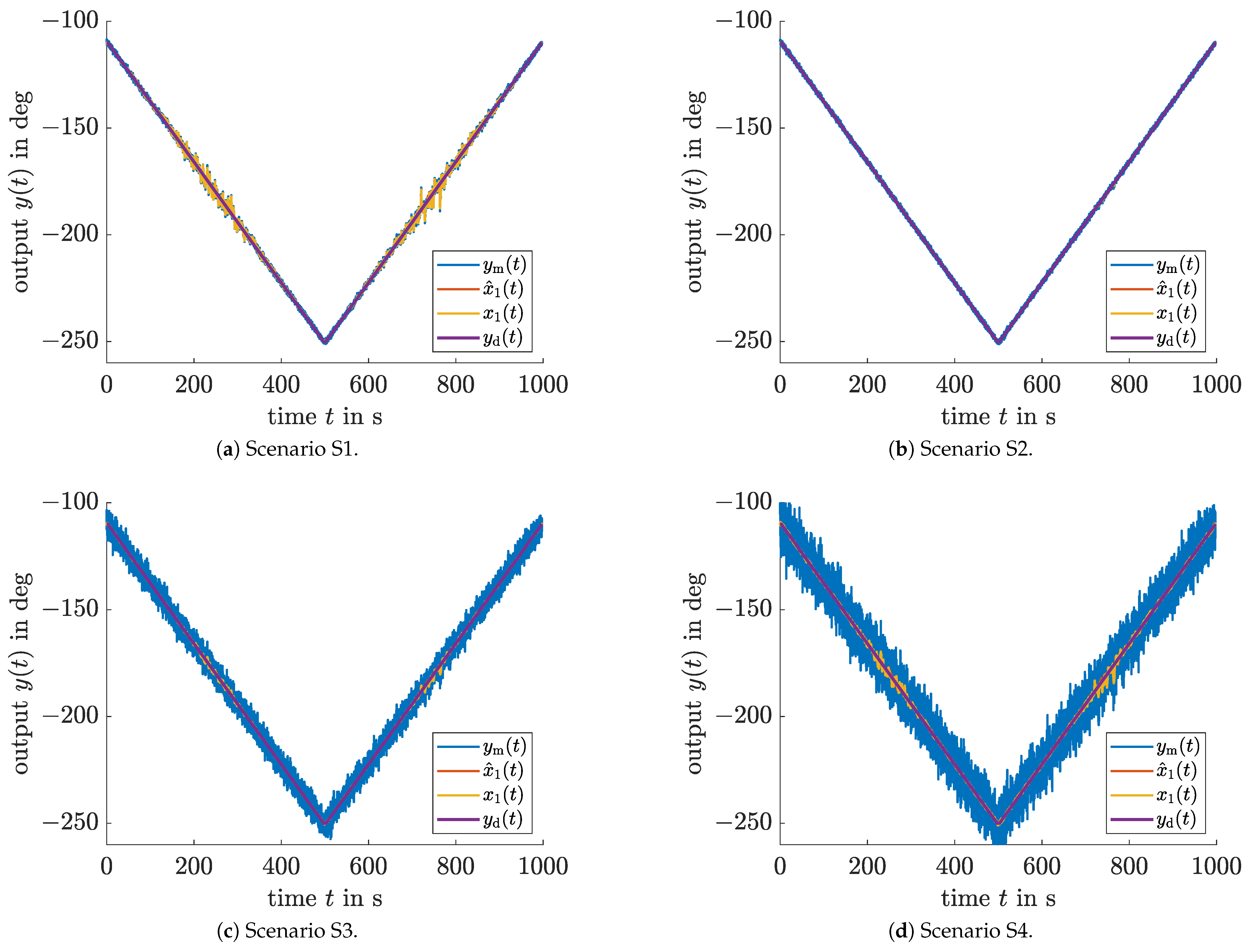
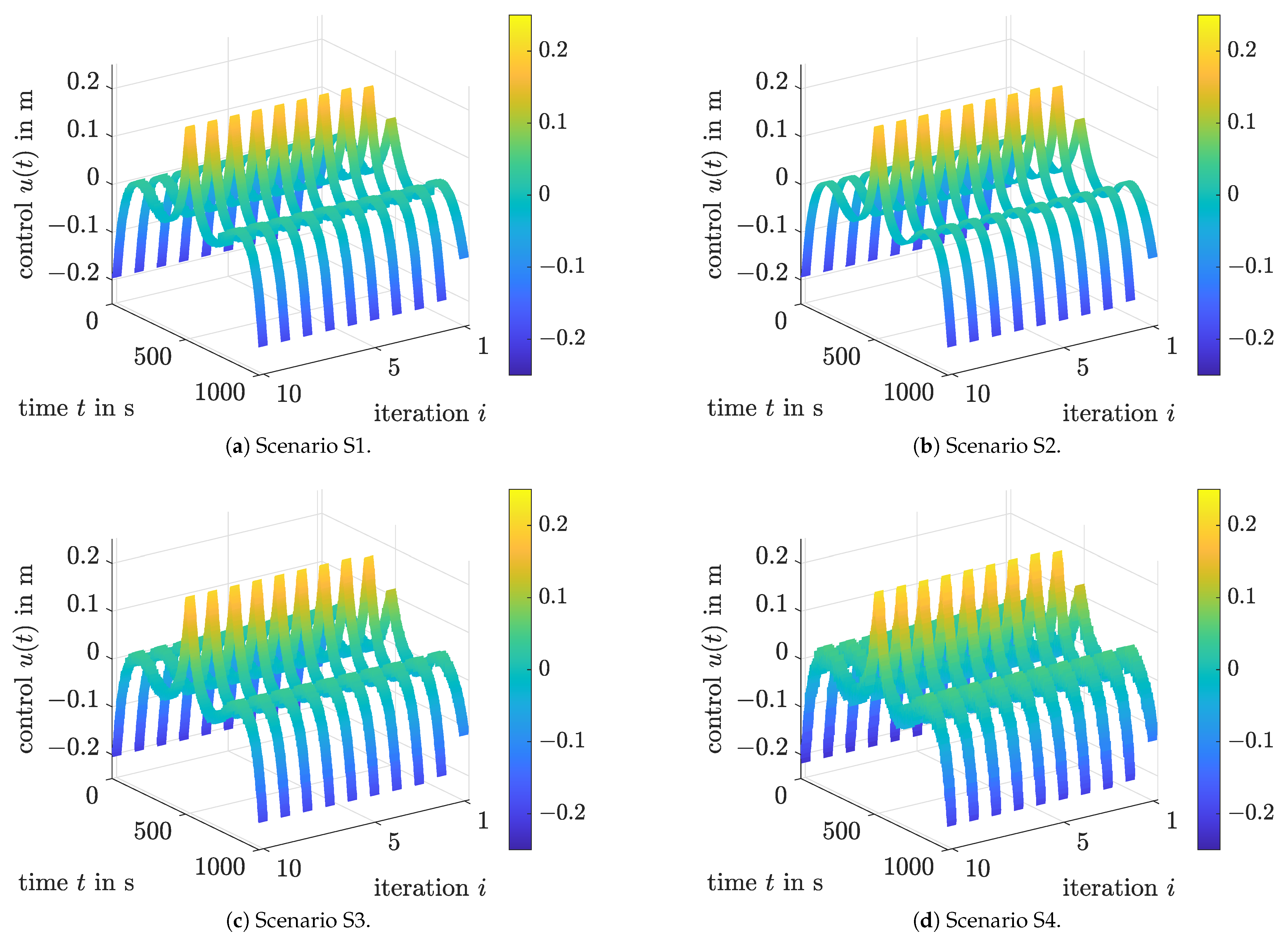
5.3. Trajectory Tracking Control

As a second application for the proposed LMI-based parameterization of the control laws (10), Case 1, and (12), Case 2, and its comparison with the LQG design, consider the following four scenarios:

S1: 

${\mathbf{G}}_{\mathrm{p}}={10}^{-2}·\mathbf{I}$, $g_u=2·{10}^{-2}\mathrm{m}$, $g_{\mathrm{m}}={10}^{-2}\mathrm{rad}\approx 0.573\mathrm{deg}$;

S2: 

${\mathbf{G}}_{\mathrm{p}}={10}^{-2}·\mathbf{I}$, $g_u=0\mathrm{m}$, $g_{\mathrm{m}}={10}^{-2}\mathrm{rad}\approx 0.573\mathrm{deg}$;

S3: 

${\mathbf{G}}_{\mathrm{p}}={10}^{-2}·\mathbf{I}$, $g_u=0\mathrm{m}$, $g_{\mathrm{m}}=5·{10}^{-2}\mathrm{rad}\approx 2.865\mathrm{deg}$;

S4: 

${\mathbf{G}}_{\mathrm{p}}={10}^{-2}·\mathbf{I}$, $g_u=0\mathrm{m}$, $g_{\mathrm{m}}=10·{10}^{-2}\mathrm{rad}\approx 5.730\mathrm{deg}$.

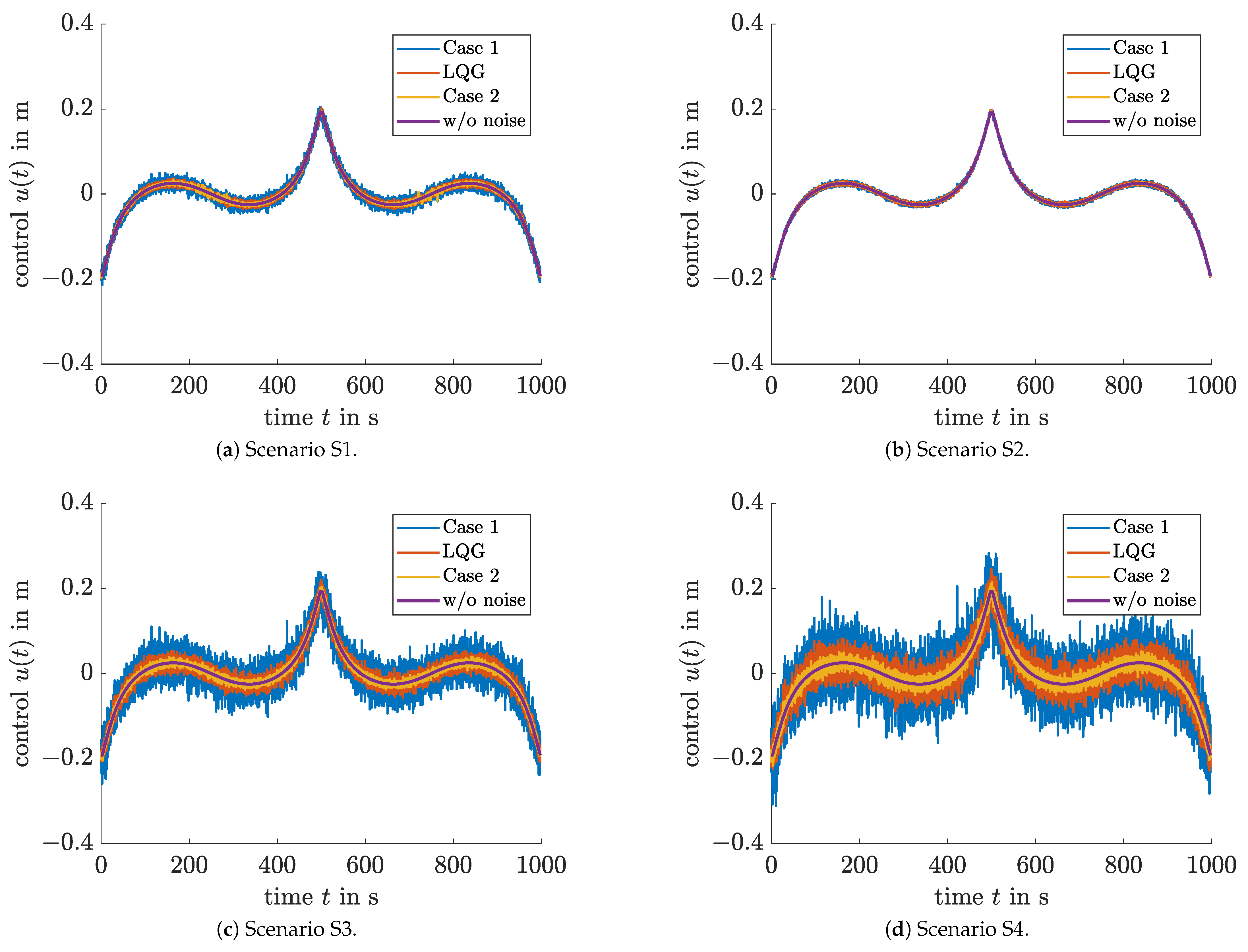
Here, we assume tracking of a continuous reference trajectory along the unstable branch of the previously investigated bifurcation diagram. Figure 5 presents a comparison of all three control approaches with an ideal tracking behavior in a noise-free setting. Obviously, the control effort of the LMI-based output feedback control is the best in all scenarios. This is achieved by minimizing the domain of non-provable stability properties and by feeding back only the first two components of the estimated state vector.

Figure 5. Comparison of the control effort for the LMI-based full state feedback controller (Case 1), the LMI-based output feedback controller (Case 2), and the LQG technique with the ideal noise-free control signal.

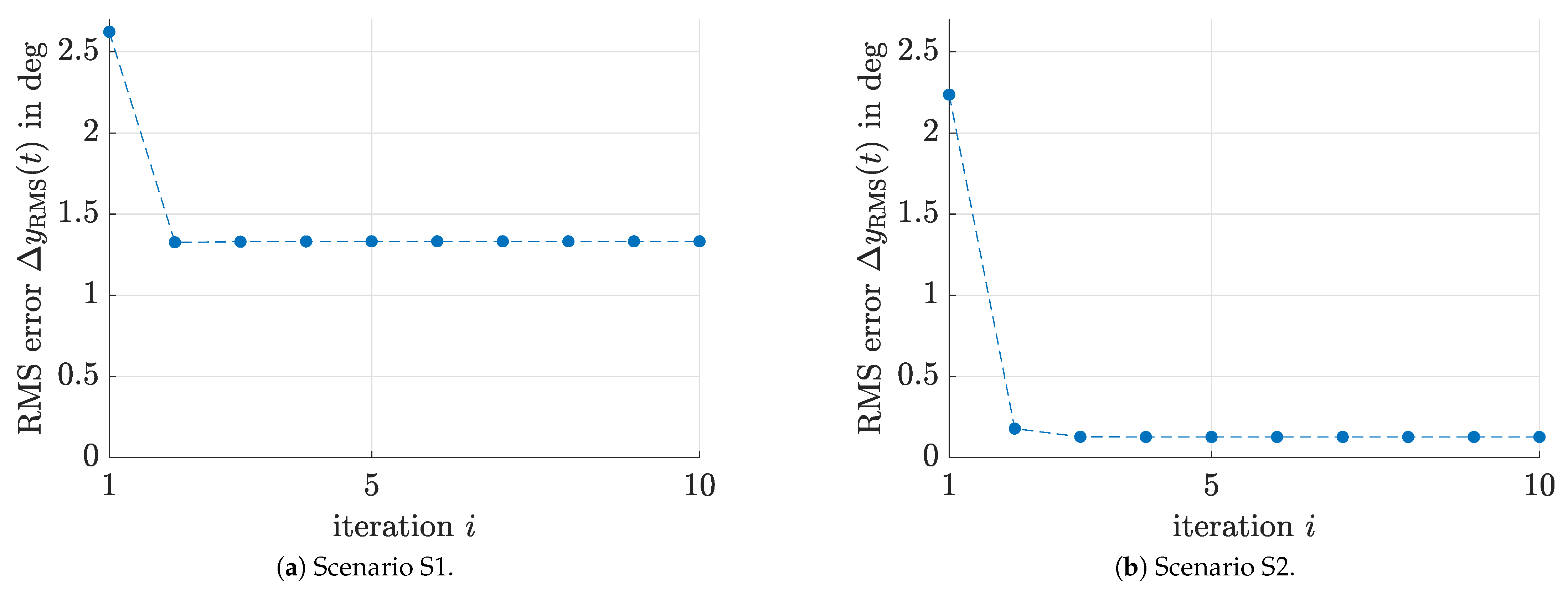
To achieve accurate tracking of the reference trajectory $y_{\mathrm{d}}$ in Figure 6, the feedforward control signal $u_{\mathrm{ff}}$ in (10) and (12) was chosen as a signal that is piecewise constant for intervals of $100\mathrm{ms}$. It is determined in the sense of a P-type iterative learning control approach by the update rule

$$u_{\mathrm{ff},i+1}\left(t_k\right)=u_{\mathrm{ff},i}\left(t_k\right)+S_k·\left(y_{\mathrm{d}}\left(t_k\right)-{\widehat{y}}_i\left(t_k\right)\right)$$

(67)

with the initialization

$$u_{\mathrm{ff},1}\left(t_k\right)=0,$$

(68)

where $u_{\mathrm{ff},i}\left(t\right)=u_{\mathrm{ff},i}\left(t_k\right)$ generally holds for $t_k\le t<t_{k+1}$. The learning gain $S_k$, weighting the difference between the observed system output ${\widehat{y}}_i\left(t_k\right)={\mathbf{C}}_{\mathrm{m}}·{\widehat{\mathbf{x}}}_i\left(t_k\right)$ in the iteration i and the reference signal, is given by

$$S_k={\left({\mathbf{C}}_{\mathrm{m}}·{\left(-{\mathbf{A}}_k+{\mathbf{B}}_k·\mathbf{K}\right)}^{-1}·{\mathbf{B}}_k\right)}^{-1},$$

(69)

where $\mathbf{K}$ is either the LQG controller’s gain, the full state feedback gain in (10), or $\mathbf{K}=\left[\begin{array}{cc}{\mathbf{K}}_{\mathrm{o}}& 0\end{array}\right]$ for the partial state feedback (12); ${\mathbf{A}}_k$ and ${\mathbf{B}}_k$ result from evaluating the system matrices in (61) for the current state estimate ${\widehat{\mathbf{x}}}_i\left(t_k\right)$ at the point of time $t_k$ during the epoch i (also denoted as trial or pass in the literature on iterative learning control).

Figure 6. Comparison of the output tracking behavior as well as the state reconstruction accuracy for the proposed LMI-based output feedback controller (Case 2) after the 10th iteration.

For the first iteration $i=1$, the controller

$$u_i\left(t\right)=u_{\mathrm{ff},i}\left(t\right)-k_1·\left(x_1\left(t\right)-y_{\mathrm{d}}\left(t\right)\right)-k_2{x}_2\left(t\right)-k_3{x}_3\left(t\right),$$

(70)

is identical to (66) introduced in the previous subsection due to the initialization (68).

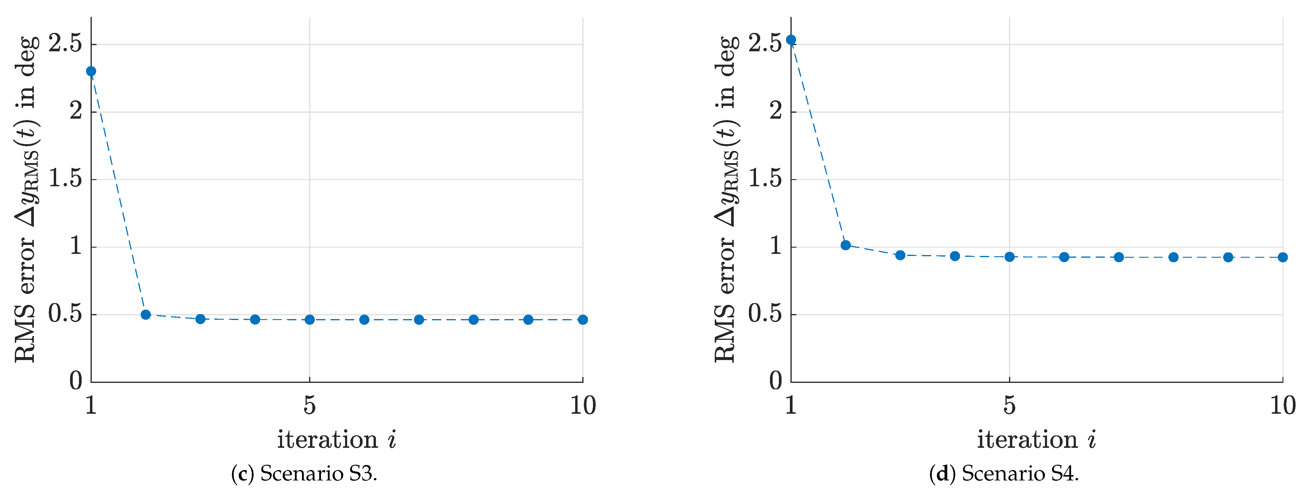
In addition to the accurate trajectory tracking for the final iteration $i=10$, Figure 6 shows the strong suppression of measurement noise by the LMI-based observer and the fact that the actual trajectories for the state $x_1$ and the corresponding estimate ${\widehat{x}}_1$ practically cannot be distinguished within the graphical resolution. Finally, Figure 7 and Figure 8 show the noise-insensitive convergence of the control signals and root mean square (RMS) output tracking errors for all four scenarios S1–S4.

Figure 7. Comparison of the control signal $u\left(t\right)$ for 10 iterations of the proposed LMI-based output feedback controller (Case 2).

Figure 8. Reduction of the output tracking error over 10 iterations for the proposed LMI-based output feedback controller (Case 2).

As a summary, all three control approaches are compared in Table 1. It can be observed that the LMI-based output feedback controller (Case 2) has the smallest deviations between the actual control signals $u_{\mathcal{S}}\left(t_k\right)$ and the ideal noise-free system inputs $u_{\mathrm{d}}\left(t_k\right)$. This is shown by a reduction of the RMS values

$$\Delta u_{\mathcal{S},\mathrm{RMS}}=\sqrt{\frac{1}{N}\sum _{k=1}^N{\left(u_{\mathcal{S}}\left(t_k\right)-u_{\mathrm{d}}\left(t_k\right)\right)}^2}$$

(71)

of the system inputs by more than $30\%$ in all scenarios $\mathcal{S}\in \{S1,\dots ,S4\}$, in comparison with the LQG implementation. These RMS values are evaluated on an equidistant discretization grid with $t_{k-1}-t_k=100\mathrm{ms}$ leading to $N\approx {10}^4$.

Table 1. Comparison of tracking errors and control effort of all controllers for the scenarios S1–S4 in terms of the root mean square deviations to an ideal noise-free trajectory tracking; the control improvement is quantified by a comparison of Case 2 with the LQG in terms of $\Delta u_{\mathrm{RMS}}$.

Scenario	Case 1		Case 2		LGQ		Control Improve-
	$\mathbf{\Delta }{\mathit{y}}_{\mathbf{RMS}}/\mathbf{deg}$	$\mathbf{\Delta }{\mathit{u}}_{\mathbf{RMS}}/\mathbf{m}$	$\mathbf{\Delta }{\mathit{y}}_{\mathbf{RMS}}/\mathbf{deg}$	$\mathbf{\Delta }{\mathit{u}}_{\mathbf{RMS}}/\mathbf{m}$	$\mathbf{\Delta }{\mathit{y}}_{\mathbf{RMS}}/\mathbf{deg}$	$\mathbf{\Delta }{\mathit{u}}_{\mathbf{RMS}}/\mathbf{m}$	ment in %
S1	$0.945$	$0.0083$	$1.332$	$0.0027$	$0.713$	$0.0040$	$33.25$
S2	$0.091$	$0.0030$	$0.1275$	$0.0009$	$0.092$	$0.0021$	$56.51$
S3	$0.339$	$0.0246$	$0.463$	$0.0047$	$0.364$	$0.0106$	$55.95$
S4	$0.636$	$0.0425$	$0.925$	$0.0090$	$0.705$	$0.0211$	$57.59$

Moreover, the full state feedback according to Case 1 has a quality comparable to that of the classical LQG in terms of the control amplitudes as well as the output RMS values

$$\Delta y_{\mathcal{S},\mathrm{RMS}}=\sqrt{\frac{1}{N}\sum _{k=1}^N{\left(x_{1,\mathcal{S}}\left(t_k\right)-y_{\mathrm{d}}\left(t_k\right)\right)}^2},$$

(72)

where $x_{1,\mathcal{S}}\left(t_k\right)$ is the simulated first state variable in the respective scenario $\mathcal{S}$. However, in comparison to the LQG, it possesses a strict proof of stability despite the polytopic parameter uncertainty, which makes the separation principle invalid as discussed in Section 2. Concerning Case 2, which is less accurate concerning output tracking than the full state feedback, it should be pointed out that the RMS output values are significantly smaller than the standard deviations of the measurement noise, except for scenario S1, where a large additive disturbance acts directly on the control input.

From a practical point of view, it is necessary to make a trade-off between tracking accuracy and control effort. Using the presented approach, the partial state feedback (Case 2) reduces the control effort in comparison to the full state feedback (Case 1), however, with the cost of a slight decrease in tracking accuracy.

6. Conclusions and Outlook on Future Work

In this paper, a novel iterative LMI solution for the joint control and observer parameterization of systems with polytopic parameter uncertainty and stochastic process, actuator, and sensor noise was derived. It is, by construction, equally applicable to the design of observer-based state and output feedback approaches. Most importantly, it allows for a guaranteed stabilization of the system dynamics despite bounded (polytopic) uncertainty in the system matrices, which makes the classical separation principle of control and observer design invalid. It was shown in benchmark simulations that the approach outperforms an LQG design for which a point-valued system model was used for the underlying controller and observer parameterization and, therefore, does not guarantee stability by design.

In future work, this approach will be further investigated for discrete-time processes. Moreover, it is desired to optimize the structure of output feedback controllers and reduced-order observers for high-dimensional systems such that the number of variables that are required for a robust parameterization is minimized. Finally, we aim at introducing and optimizing weighting factors for the diagonal entries in the matrix (47) so that, during the minimization of (41), the user can decide which of the individual states (or estimation error signals) has the highest importance. This extension will have similarities to tuning the ratio between the weighting matrix entries for state deviations in the classical LQR design.