Interval Extended Kalman Filter—Application to Underwater Localization and Control

Abstract

The extended Kalman filter has been shown to be a precise method for nonlinear state estimation and is the facto standard in navigation systems. However, if the initial estimated state is far from the true one, the filter may diverge, mainly due to an inconsistent linearization. Moreover, interval filters guarantee a robust and reliable, yet unprecise and discontinuous localization. This paper proposes to choose a point estimated by an interval method, as a linearization point of the extended Kalman filter. We will show that this combination allows us to get a higher level of integrity of the extended Kalman filter.

1. Introduction

The dynamic of a mobile robot is generally described by the following discrete time nonlinear state equation

$$\left\{\begin{array}{cc}{\mathbf{x}}_{k+1}\hfill & ={\mathbf{f}}_k({\mathbf{x}}_k,{\mathbf{u}}_k,{\mathbf{n}}_k)\hfill \\ {\mathbf{y}}_k\hfill & ={\mathbf{g}}_k\left({\mathbf{x}}_k\right)+{\nu }_k\hfill \end{array}\right.$$

(1)

where $k\in \mathbb{N}$ is the time, ${\mathbf{x}}_k\in {\mathbb{R}}^n$ is the state vector, ${\mathbf{u}}_k$ is the input vector, ${\mathbf{n}}_k$ is the state noise, ${\nu }_k$ is the measurement noise, and ${\mathbf{y}}_k$ is the measured output vector. Two approaches are generally considered to solve the corresponding state estimation problem:

• The probabilistic approach [1,2] is over-optimistic and might converge to some fake states. In most of the cases, the implementation relies on an extended Kalman filter (EKF) [3], which is efficient and accurate.
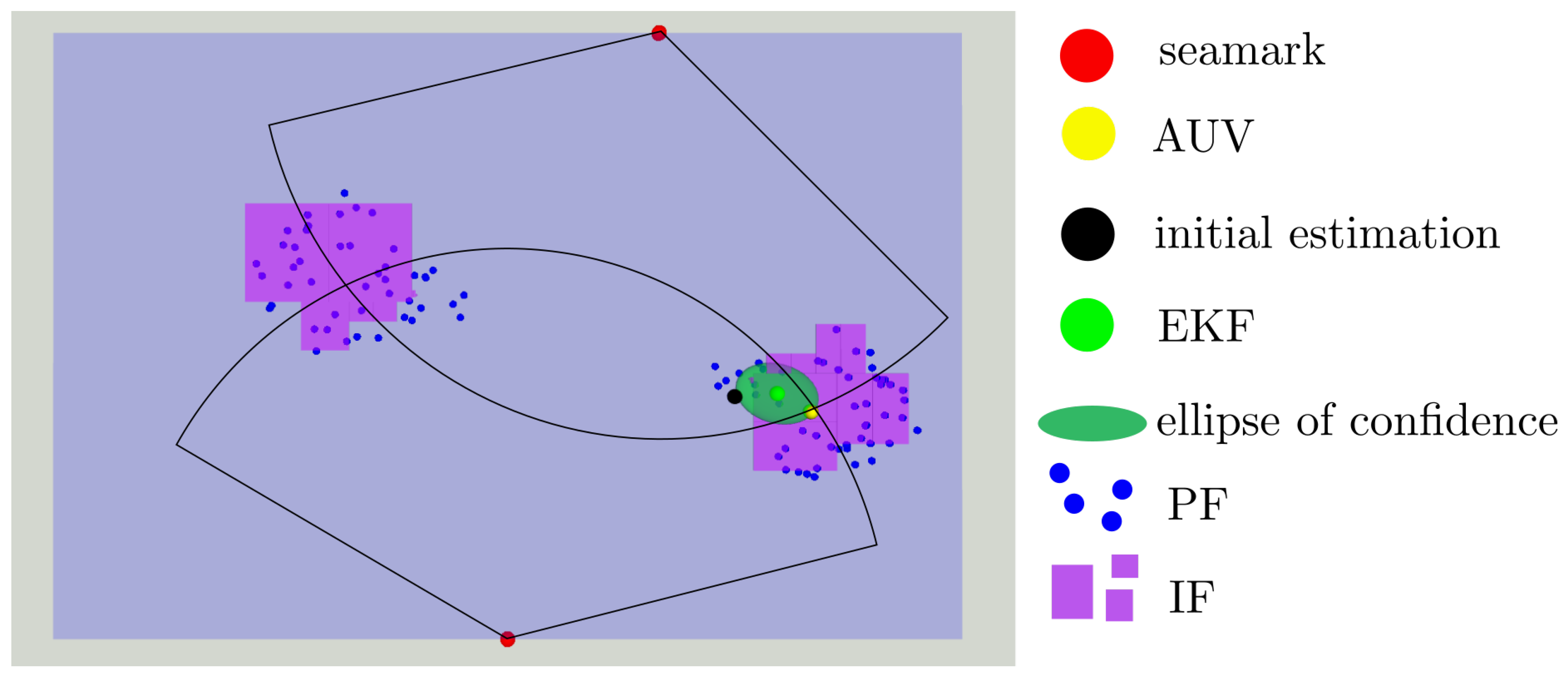
• The set membership approach [4] is over-pessimistic. Its principle is to discard states [5] that are inconsistent with the collected data. Since no consistent state is rejected, these approaches have a high level of integrity [6,7], even if they are considered are not precise. Usually, the implementation uses interval analysis and leads to what we can call an interval filter (IF) [8].

The main reason why an EKF may converge toward a fake state is that the linearization point that is chosen can be far from the true state [1]. Moreover, this linearization point, taken from the Kalman filter itself, can be totally inconsistent and would thus have been rejected by the interval filter. The idea we want to develop here is to select a linearization point inside the feasible set generated by an interval filter. Of course, this consistent point could still be far from the true one, but we understand that this choice reduces the possibility of bad behavior of the observer. The resulting controller would not be a hybrid between an IF and an EKF, but rather an EKF helped by the IF for the linearization.

The idea of combining probabilities with interval-based methods to have a method which is both safe and accurate is not new. It is the objective of the box particle filter [9,10] and other filters such as [11,12], which combines particle filters with set-membership methods. It is also the objective of the interval Kalman filter [13], which add interval analysis to bound uncertainties in the Kalman Filter. Using a better Kalman filter such as the unscented Kalman filter (UKF) [2] would give better performances than the EKF, but could still converge toward a fake state because of the linearization point. Moreover, it is possible to use a particle filter (PF) [1] instead of the interval filter since it is also a global method. We decided to use the IF because this method has more integrity and generally requires less computations.

The paper is organized as follows. Section 2 gives a 2D overview of the different filters and the linearization problem. Section 3 provides the three filters to be used: the Extended Kalman filter (EKF), the Interval Filter (IF), and the Interval Extended Kalman Filter (IEKF). Section 4 and Section 5 compare the three approaches (EKF, IF, IEKF) on the localization problem of an underwater robot for different scenarios. Section 6 concludes the paper.

2. Introductory Problem

To introduce the linearization problem and the interest of different filters, here is an example of a static 2D localization problem of an AUV:

This AUV is on the surface of a rectangle lake. It is not moving, and it can measure its distance to two seamarks with some noise. Figure 1 shows the estimation of different filters with one measurement. Since the IF and the PF are global methods, they reveal the two zones that are coherent with the measurements. Moreover, the EKF give an estimation with a better precision if the initial estimation—which is also the linearization point—is close to the right zone. However, if the initial estimation was close to the left zone, the EKF would have converged toward that latter.

3. Filters

3.1. Extended Kalman Filter

The extended Kalman filter (EKF) is the nonlinear version of the Kalman filter, which linearizes the observed system through an estimate of the current mean and covariance. It obeys the following equations:

$$\begin{array}{ccc}{\mathbf{C}}_k\hfill & ={\displaystyle \frac{\partial {\mathbf{g}}_k\left({\overline{\mathbf{x}}}_k\right)}{\partial \mathbf{x}}}\hfill & (\mathrm{observation}\mathrm{matrix})\hfill \\ {\tilde{\mathbf{z}}}_k\hfill & ={\mathbf{y}}_k-{\mathbf{g}}_k\left({\widehat{\mathbf{x}}}_k\right)\hfill & \left(\mathrm{innovation}\right)\hfill \\ {\mathbf{S}}_k\hfill & ={\mathbf{C}}_k{\mathsf{\Gamma }}_k{\mathbf{C}}_k+{\mathsf{\Gamma }}_{{\mathit{\beta }}_k}\hfill & (\mathrm{covariance}\mathrm{of}\mathrm{the}\mathrm{innovation})\hfill \\ {\mathbf{K}}_k\hfill & ={\mathsf{\Gamma }}_k{\mathbf{C}}_k{\mathbf{S}}_k\hfill & (\mathrm{Kalman}\mathrm{gain})\hfill \\ {\mathbf{A}}_k\hfill & ={\displaystyle \frac{\partial {\mathbf{f}}_k}{\partial \mathbf{x}}}({\overline{\mathbf{x}}}_k+{\mathbf{K}}_k{\tilde{\mathbf{z}}}_k,{\mathbf{u}}_k)\hfill & (\mathrm{evolution}\mathrm{matrix})\hfill \\ {\widehat{\mathbf{x}}}_{k+1}\hfill & ={\mathbf{f}}_k({\widehat{\mathbf{x}}}_k+{\mathbf{K}}_k{\tilde{\mathbf{z}}}_k,{\mathbf{u}}_k)\hfill & (\mathrm{predicted}\mathrm{estimation})\hfill \\ {\mathsf{\Gamma }}_{k+1}\hfill & ={\mathbf{A}}_k(\mathbf{I}-{\mathbf{K}}_k{\mathbf{C}}_k){\mathsf{\Gamma }}_k{\mathbf{A}}_k+{\mathsf{\Gamma }}_{{\alpha }_k}\hfill & (\mathrm{predicted}\mathrm{covariance})\hfill \end{array}$$

(2)

The covariance matrices of the noises are written ${\mathsf{\Gamma }}_{{\alpha }_k}$ and ${\mathsf{\Gamma }}_{{\mathit{\beta }}_k}$. These covariance matrices are used to estimate the covariance of the estimated state regarding the uncertainty given by the process and the measurement noises. However, they do not take into account model uncertainty, and linearization errors. They are set empirically. The EKF is initialized with the initial state guess ${\widehat{\mathbf{x}}}_0$ and the initial state covariance matrix ${\mathsf{\Gamma }}_0$. At every iteration, it takes as inputs ${\widehat{\mathbf{x}}}_k$, ${\mathsf{\Gamma }}_k$, ${\mathbf{y}}_k$ and ${\mathbf{u}}_k$ and returns ${\widehat{\mathbf{x}}}_{k+1}$, and ${\mathsf{\Gamma }}_{k+1}$.

In the classical EKF, the linearization point ${\overline{\mathbf{x}}}_k$ is taken as ${\widehat{\mathbf{x}}}_k$, the state estimation computed by the EKF at the previous step. During the initialization, ${\widehat{\mathbf{x}}}_0$ can be far from the true state ${\mathbf{x}}_0$, and the linearization errors might be huge [3,14]. Since this linearization cannot be taken into account by the EKF, the filter can be attracted by a fake state away from the true one.

3.2. Interval Filter

The interval filter [15,16] (IF) we propose to consider here is based on interval analysis [17,18]. The observer provides a set represented by a union of non-overlapping boxes. This union is guaranteed to contain the true state. The principle of the IF is to remove zones of the state space that contain only inconsistent values. It is known to be over-pessimistic. However, it has a high level of integrity, since it allows us to take into account many types of errors such as the linearization errors [19,20,21], the discretization errors of the differential state Equation [22,23,24,25], and the measurement noise [4,26,27,28].

At each iteration of Equation (1), the noises are assumed to be in the boxes $\left[{\mathbf{n}}_k\right]$ and $\left[{\nu }_k\right]$, and the state is known to be in the box $\left[{\mathbf{x}}_k\right]$. Moreover, the input ${\mathbf{u}}_k$ and output ${\mathbf{y}}_k$ are known to belong to the boxes $\left[{\mathbf{u}}_k\right]$ and $\left[{\mathbf{y}}_k\right]$. Therefore a Forward-Backward contraction $C_y$ is designed for the measurement equation and has the Algorithm 1 given by [29]:

Algorithm 1:Algorithm of $C_y$ at the iteration k

Input: the boxes $\left[{\mathbf{x}}_k\right],\left[{\mathbf{y}}_k\right],\left[{\nu }_k\right]$ Output: the same updated boxes $\begin{array}{cc}\left[\mathbf{a}\right]={\mathbf{g}}_k\left(\left[{\mathbf{x}}_k\right]\right)\hfill & //\mathbf{a}={\mathbf{g}}_k\left({\mathbf{x}}_k\right)\\ \left[\mathbf{a}\right]=\left[\mathbf{a}\right]\cap \left[{\mathbf{y}}_k\right]-\left[{\nu }_k\right]\hfill & //\mathbf{a}={\mathbf{y}}_k-{\nu }_k\\ \left[{\mathbf{x}}_k\right]=\left[{\mathbf{x}}_k\right]\cap {\mathbf{g}}_k^{-1}\left(\left[\mathbf{a}\right]\right)\hfill & //{\mathbf{x}}_k={\mathbf{g}}_k^{-1}\left(\mathbf{a}\right)\\ \left[{\mathbf{y}}_k\right]=\left[{\mathbf{y}}_k\right]\cap \left[\mathbf{a}\right]+\left[{\nu }_k\right]\hfill & //{\mathbf{y}}_k=\mathbf{a}+{\nu }_k\\ \left[{\nu }_k\right]=\left[{\nu }_k\right]\cap \left[\mathbf{a}\right]-\left[{\mathbf{y}}_k\right]\hfill & //{\nu }_k=\mathbf{a}-{\mathbf{y}}_k\end{array}$

To enhance the estimation of $\left[{\mathbf{x}}_k\right]$, the box is contracted and sub-paved several times. This results in a list of N non-overlapping boxes $L_{x,k}=\left\{\left[{\overline{\mathbf{x}}}_k\right]|i\in ⟦1:N⟧\right\}$, with one box containing the real value of ${\mathbf{x}}_k$. Then, for the next iteration, $\left[{\mathbf{x}}_{k+1}\right]$ can be initially estimated as the box containing all the boxes obtained from $L_{x,k}$ by dead reckoning:

$$\left[{\mathbf{x}}_{k+1}\right]=\underset{i\in ⟦1:N⟧}{\cup }\left(\mathbf{f}\left(\left[{\overline{\mathbf{x}}}_k\right],\left[{\mathbf{u}}_k\right],\left[{\mathbf{n}}_k\right]\right)\right)$$

(3)

This localization is robust, since the state is guaranteed to be in one of the box of the list $L_{x,k}$. Then in a closed loop system relying on state estimation, the controller is expecting an estimated vector ${\widehat{\mathbf{x}}}_k$ and not a box. Thus, we have to select one point in the set $L_{x,k}$. Since the sub-paving can be scattered in different groups, this choice can be difficult and will probably yield time discontinuities of the estimation. For example, the estimated state can be chosen as the center of the biggest box. For all types of choices, the trajectory estimated by the IF is discontinuous and less precise than the one given by the EKF, in case of good behavior.

3.3. Interval Extended Kalman Filter

Since the EKF can diverge if the linearization point is far from the real state, we propose a new observer called IEKF (Interval EKF). This filter consists of an interval filter and an extended Kalman filter. The interval filter helps the second filter by taking as a linearization point ${\overline{\mathbf{x}}}_k$, a point inside the list of boxes $L_{x,k}$. This point can be, for instance, the center of one of the boxes in $L_{x,k}$, which maximizes the consistency with respect to the observations. Now, ${\overline{\mathbf{x}}}_k$ may also be the estimate given by the IEKF when the latter is consistent enough.

Here, the IEKF corresponds to a classical EKF helped by an IF: it uses a consistency approach to select the linearization point. As a result, it will behave as a classical EKF as soon as we are close to the true solution, and the trajectory will be smooth and precise as shown in the following section. Now, when the estimated trajectory is far from the true solution, the IEKF will benefit from the global view provided by set-membership approach. The resulting observer will inherit both from the accuracy of EKF near to the solution and also to the high level of integrity provided by the IF.

4. Test-Cases

In this section, we propose to compare the three localization methods presented in Section 3.

For this, we consider an autonomous underwater vehicle (AUV), the Riptide, represented by Figure 2. For its locomotion, this robot uses three fins and one propeller. The inputs are $u_0$, the rotation speed of the propeller and the angles $u_1,u_2,u_3$ of the fins. We assume that we have no side slip effect. This means that the velocity vector ${\mathbf{v}}_r$ has always the direction of the robot, or equivalently, the robot has no lateral speed.

For each vector $\mathbf{w}=(w_x,w_y,w_z)$, we may associate the skew-symmetric matrix:

$$\mathbf{w}\wedge =\left(\begin{array}{ccc}0& -w_z& w_y\\ w_z& 0& -w_x\\ -w_y& w_x& 0\end{array}\right)$$

The state space equation of the robot is given by [30] with an adaptation in the orientation variables:

$$\left\{\begin{array}{cc}\dot{\mathbf{p}}\hfill & =\mathbf{R}·{\left(v_{r}00\right)}^T\hfill \\ \dot{\mathbf{R}}\hfill & =\mathbf{R}·({\mathbf{w}}_r\wedge )\hfill \\ {\dot{v}}_r\hfill & =q_1·u_0^2-q_2·v_r·\left|v_r\right|\hfill \\ {\mathbf{w}}_r\hfill & =v_r·\mathbf{B}·{\left(u_1{u}_2{u}_3\right)}^T\hfill \end{array}\right.$$

(4)

The Euler angles have been replaced by a rotation matrix to remove the Gimbal lock for the controller. In this model:

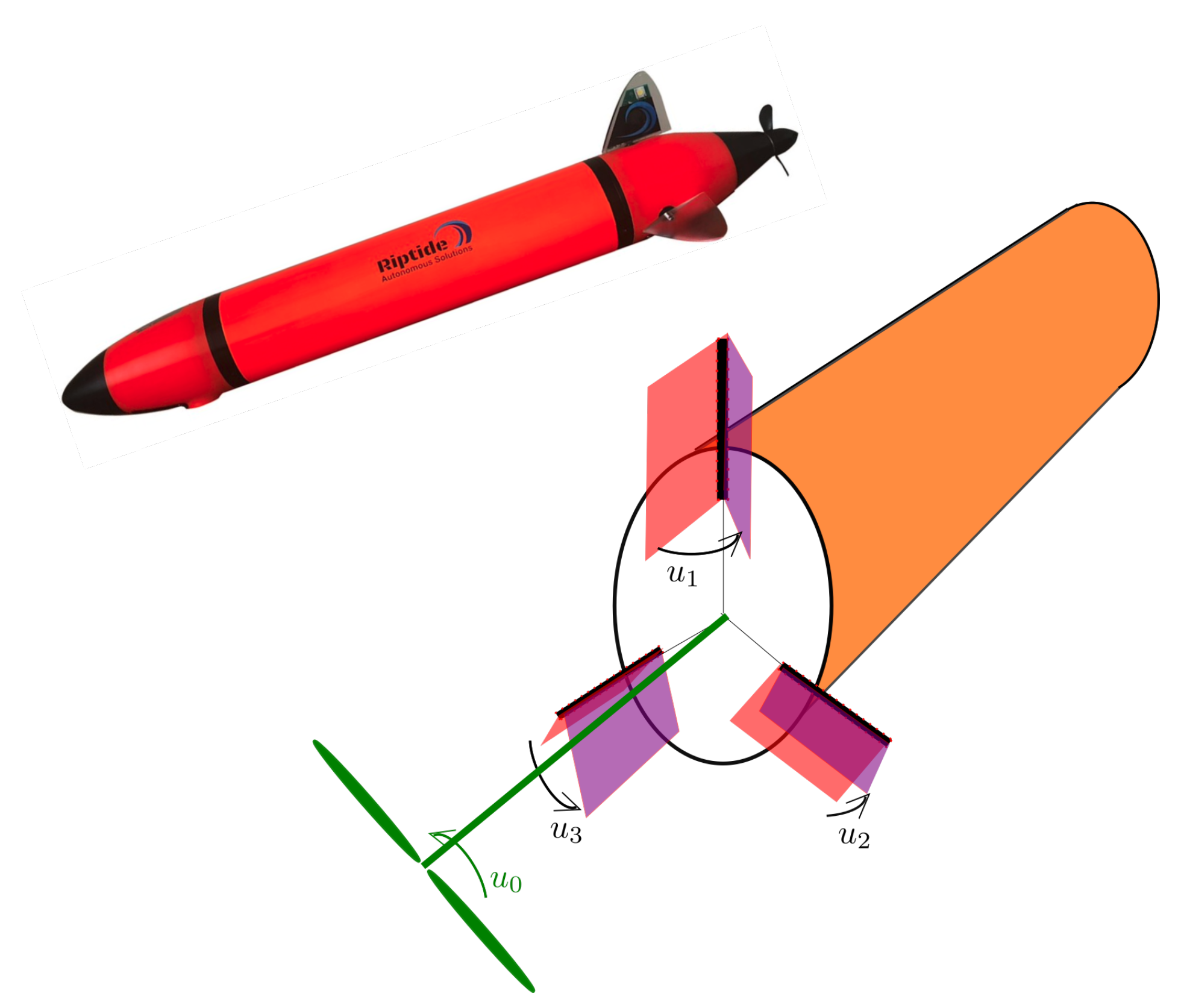
• $q_1$ and $q_2$ are known parameters. $q_1$ represents the effect of the propeller’s speed on the acceleration while $q_2$ represents the water friction.
• $\mathbf{B}$ is the known repartition matrix.
• $\mathbf{p}={(p_x,p_y,p_z)}^T$ is the position of the robot.
• $\mathbf{R}$ is the orientation matrix.
• $v_r$ is its longitudinal speed (lateral speed are supposed to be null).
• ${\mathbf{w}}_r$ is its angular speed vector.

This robot is controlled in speed and orientation with the following controller:

$$\left\{\begin{array}{cc}{u}_0\hfill & =\sqrt{{\displaystyle \frac{q_2}{q_1}}}{v}_d\hfill \\ \left(\begin{array}{c}{u}_1\\ u_2\\ u_3\end{array}\right)\hfill & ={\displaystyle \frac{1}{{\widehat{v}}_r}}{\mathbf{B}}^{-1}{\mathbf{R}}^T·\mathrm{Log}({\mathbf{R}}_d·{\mathbf{R}}^T)\hfill \end{array}\right.$$

(5)

where Log is the capitalized log map used in Lie groups theory [31]. In this controller, $v_d$ is the desired speed, the matrix ${\mathbf{R}}_d$ is the desired orientation, and ${\widehat{v}}_r$ is the estimated speed.

While $v_d$ is constant, a planner computes ${\mathbf{R}}_d$ to make the robot follow a series of connected lines. When the drone follows the line from the point ${\mathbf{a}}_j$ to the point ${\mathbf{a}}_{j+1}$ with the unit vector ${\mathbf{x}}_j$ and is on the line, it should have the specified orientation ${\mathbf{R}}_d={\mathbf{R}}_j$. Then, when the robot is at a distance e from the line, the desired orientation is rotated towards the line with the angle:

$${\theta }_e=arctan\left(e\right)$$

Moreover, the distance between the robot and the line e and the projection point ${\mathbf{p}}_l$ are calculated from the estimation of the position $\widehat{\mathbf{p}}$:

$$\left\{\begin{array}{cc}{\mathbf{p}}_l\hfill & ={\mathbf{a}}_j+<\widehat{\mathbf{p}}-{\mathbf{a}}_j|{\mathbf{x}}_j>·{\mathbf{x}}_j\hfill \\ e\hfill & =\left|\right|{\mathbf{p}}_l-\widehat{\mathbf{p}}{\left|\right|}_2\hfill \end{array}\right.$$

(6)

with the scalar product $<·|·>$ associated with the euclidean norm $\left|\right|·{\left|\right|}_2$. Then, the desired orientation matrix is set to:

$${\mathbf{R}}_d=exp({\theta }_e·{\mathbf{w}}_e\wedge )·{\mathbf{R}}_j$$

with the orthogonal vector ${\mathbf{w}}_e={\mathbf{x}}_k\wedge ({\mathbf{p}}_l-\widehat{\mathbf{p}})/\left|\right|{\mathbf{p}}_l-\widehat{\mathbf{p}}{\left|\right|}_2$.

The planner needs an estimation of the position of the drone $\widehat{\mathbf{p}}$. Therefore, an observer is designed to solve the following continuous localization problem. It is based on the following evolution model:

$$\dot{\mathbf{x}}={\mathbf{f}}_{\mathbf{c}}(\mathbf{x},\mathbf{u})=\left(\begin{array}{c}{R}_{11}{v}_r\\ R_{21}{v}_r\\ q_1·u_0^2-q_2·v_r·\left|v_r\right|\end{array}\right)$$

(7)

which corresponds to a selection of the equations of the complete model (4) that are needed for the localization. In this model, the state vector is $\mathbf{x}={(p_x,p_y,v_r)}^T$, the input is the propeller speed $u_0$. $R_{11}$ and $R_{21}$ are the two first elements of the first column of $\mathbf{R}$.

The observation equation given by

$$\mathbf{y}=\mathbf{g}\left(\mathbf{x}\right)+\mathit{\beta }=\left(\begin{array}{c}{p}_z\\ ∥\mathbf{p}-{\mathbf{m}}_1∥\\ ∥\mathbf{p}-{\mathbf{m}}_2∥\end{array}\right)+\mathit{\beta }$$

(8)

corresponds to a situation where the robot measures its depth $p_z$ and the Euclidean distances to two fixed markers ${\mathbf{m}}_1,{\mathbf{m}}_2$. The measurement noise is denoted by $\mathit{\beta }$. We assume that the orientation matrix $\mathbf{R}$ is measured with a high accuracy.

Let us discretize the state equations with an Euler method:

$$\left\{\begin{array}{cc}{\mathbf{x}}_{k+1}\hfill & ={\mathbf{x}}_k+dt·{\mathbf{f}}_c({\mathbf{x}}_k,{\mathbf{u}}_k)={\mathbf{f}}_k({\mathbf{x}}_k,{\mathbf{u}}_k)\hfill \\ {\mathbf{y}}_k\hfill & =\mathbf{g}\left({\mathbf{x}}_k\right)+{\mathit{\beta }}_k={\mathbf{g}}_k\left({\mathbf{x}}_k\right)+{\mathit{\beta }}_k\hfill \end{array}\right.$$

(9)

with the sampling time $dt=0.1s$ which has the same form than Equation (1) without process noise. That discretization will be used by the extended Kalman filters. The three localization methods have been implemented for this problem. Figure 3 shows the block diagram of the closed loop system. The IEKF provides the estimates $\widehat{\mathbf{p}}$ and ${\widehat{v}}_r$.

The three localization methods are then compared with a closed loop simulation where the system is simulated with the same Euler discretization (the Runge-Kutta methods have shown similar results). Two scenarios are simulated with two different initial positions for the robot:

• In the first one, the initial estimation of the position of the robot has an error of 1 m.
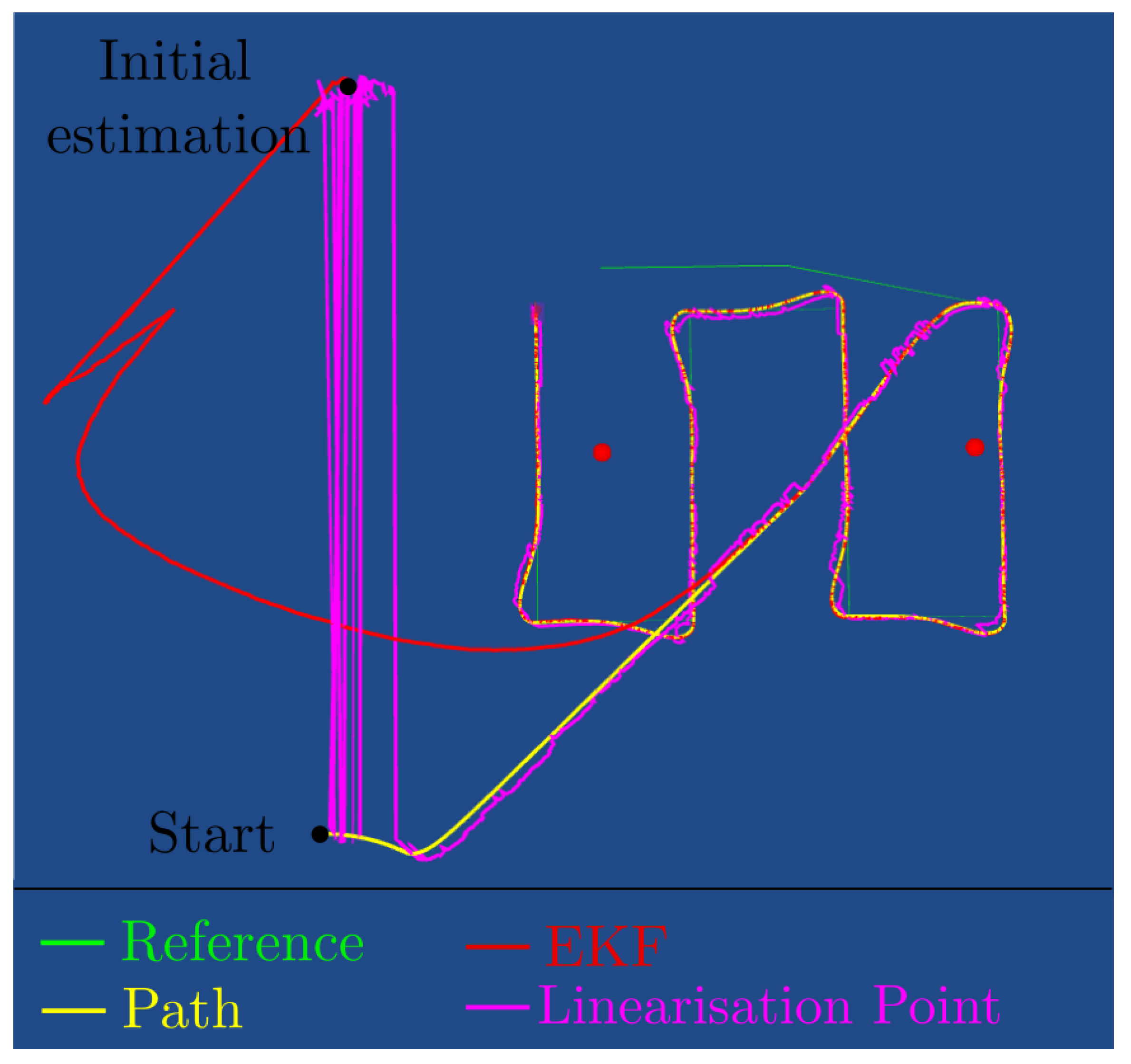
• In the second one, the initial position is chosen to make the Extended Kalman Filter diverge. The initial error is large, approximately 23 m (see Figure 7).

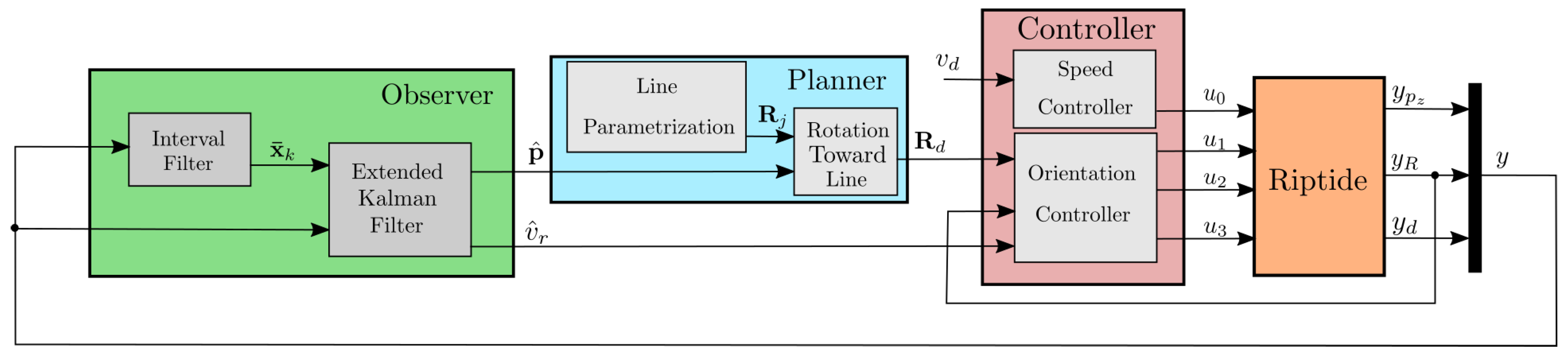
5. Simulation Results

Figure 4, Figure 5, Figure 6, Figure 7, Figure 8 and Figure 9 show the results of these simulations in the context of line following of an AUV. These Figures are screenshots of the trajectories from above. The objective of the AUV is to follow the green path. The yellow path is the real path of the robot. The magenta is the localization by interval analysis. The red is the localization with the Kalman filter. The two red circles are the markers and are 20 m away from each other.

In addition, an animation of the second scenario with the modified extended Kalman filter is available (https://youtu.be/tdkt9DJLPo8, accessed on 12 March 2021). In this video, the magenta boxes represent the estimation boxes from interval analysis, and the red ellipse is the ellipse of confidence of the Kalman filter. In the transition phase where the speed estimation is not accurate yet, the dead reckoning may put the drone out of the box. Yet, after the transition phase, the drone is always in the confidence box from interval analysis. Moreover, after the convergence of the Kalman filter, the robot is also in the ellipse of confidence.

5.1. Interval Analysis Observer

Regarding the Interval Analysis Observer, its performances are similar in both scenarios (see Figure 4 and Figure 7). At the beginning of the simulation, the Interval Filter estimates two coherent sets (see the sets a and b in Figure 7). Figure 10 details this behavior. The robot is in position ${\mathbf{p}}_1$, and then moves to position ${\mathbf{p}}_2$. While the robot is in ${\mathbf{p}}_1$, the contraction and sub-paving result in two sets of solutions, the magenta boxes. As a consequence, the estimated position can jump from one to the other set. However when the robot reaches ${\mathbf{p}}_2$, the bottom magenta box move to the black box by dead reckoning and then contracts to an empty box. Meanwhile, the top magenta box moves and contract into the yellow box, giving a better estimation of the robot’s position.

Then, in Figure 4 and Figure 7, the estimated position (magenta) follows the true position (yellow) with a precision of about 1m and with small jumps. Therefore, this localization is not optimal, but robust in the two scenarios.

5.2. Extended Kalman Filter

Figure 5 shows that in the right scenario, the localization with the Extended Kalman Filter is more precise than interval analysis. Indeed, the estimated position is visually close to the real position. However, in the second scenario (see Figure 8), the Kalman filter diverges because there is another local minimum for the covariance. Furthermore, this local minimum is closer to the estimated position than the real position. So this filter is more precise, but not robust.

5.3. Extended Kalman Filter with Interval Analysis

Figure 6 shows a localization similar to Figure 5. Indeed, in this case, the localization points of the two Kalman filters are close to each other. However, in Figure 6, the localization jumps of the interval analysis has an impact on the Kalman filter in the initial transition phase. Nevertheless, in the second scenario Figure 9, instead of diverging, the interval extended Kalman filter converge towards the real position of the drone after the transition phase.

6. Conclusions

The probabilistic and the set membership approaches in the localization problems are often seen as different and in competition. In this paper, we have shown that they may collaborate to keep both the integrity of the interval filter and the accuracy of the Kalman filter.

While in practice, the robots often rely on a probabilistic localization with a Kalman Filter for their online autonomous navigation, the set membership method is mainly used in post-process analysis. This paper proposes a new filter IEKF which benefits from the advantages of the EKF and the IF. By linearizing the EKF at a point given by the IF, the IEKF is more likely to converge. Moreover, the IF can be used to verify the consistency of the observer, and validate that the robot did not enter inside a forbidden zone.

Of course, our filter requires more computation with two observers instead of one, but it is the prize to pay if we want both the integrity needed to a safe navigation and the accuracy, needed to have smooth trajectories that do not overload the actuators too much.

References

- Thrun, S.; Bugard, W.; Fox, D. Probabilistic Robotics; MIT Press: Cambridge, MA, USA, 2005. [Google Scholar]
- Julier, S.; Uhlmann, J. Unscented filtering and nonlinear estimation. Proc. IEEE 2004, 92, 401–422. [Google Scholar] [CrossRef]
- Ljung, L. Asymptotic Behavior of the Extended Kalman Filter as a Parameter Estimator for Linear Systems. IEEE Trans. Autom. Syst. 1979, 24, 36–50. [Google Scholar] [CrossRef]
- Milanese, M.; Norton, J.; Piet-Lahanier, H.; Walter, E. (Eds.) Bounding Approaches to System Identification; Plenum Press: New York, NY, USA, 1996. [Google Scholar]
- Jaulin, L.; Kieffer, M.; Didrit, O.; Walter, E. Applied Interval Analysis, with Examples in Parameter and State Estimation, Robust Control and Robotics; Springer-Verlag: London, UK, 2001. [Google Scholar]
- Drevelle, V.; Bonnifait, P. High integrity GNSS location zone characterization using interval analysis. In Proceedings of the 22nd International Technical Meeting of the Satellite Division of The Institute of Navigation (ION GNSS 2009), Savannah, GA, USA, 22–25 September 2009. [Google Scholar]
- Rauh, A.; Auer, E. Interval Approaches to Reliable Control of Dynamical Systems. In Proceedings of the Computer-Assisted Proofs—Tools, Methods and Applications, Wadern, Germany, 15–20 November 2009. [Google Scholar]
- Rohou, S.; Jaulin, L.; Mihaylova, M.; Bars, F.L.; Veres, S. Guaranteed Computation of Robots Trajectories. Robot. Auton. Syst. 2017, 93, 76–84. [Google Scholar] [CrossRef]
- Abdallah, F.; Gning, A.; Bonnifait, P. Box particle filtering for nonlinear state estimation using interval analysis. Automatica 2008, 44, 807–815. [Google Scholar] [CrossRef]
- Gning, A.; Ristic, B.; Mihaylova, L.; Abdallah, F. An Introduction to Box Particle Filtering. IEEE Signal Process. Mag. 2013, 30, 166–171. [Google Scholar] [CrossRef]
- Neuland, R.; Nicola, J.; Maffei, R.; Jaulin, L.; Prestes, E.; Kolberg, M. Hybridization of Monte Carlo and Set-membership Methods for the Global Localization of Underwater Robots. In Proceedings of the 2014 IEEE/RSJ International Conference on Intelligent Robots and Systems, Chicago, IL, USA, 14–18 September 2014; pp. 199–204. [Google Scholar]
- Neuland, R.; Mantelli, M.; Hummes, B.; Jaulin, L.; Maffei, R.; Prestes, E.; Kolberg, M. Robust Hybrid Interval-Probabilistic Approach for the Kidnapped Robot Problem. Int. J. Uncertain. Fuzziness Knowl. Based Syst. 2020, 29, 313–331. [Google Scholar] [CrossRef]
- Tran, T.; Jauberthie, C.; Trave-massuyes, L.; Lu, Q. Interval Kalman filter enhanced by lowering the covariance matrix upper bound. Ifac Pap. 2017, 50, 1595–1600. [Google Scholar] [CrossRef]
- Jaulin, L. Mobile Robotics; ISTE: London, UK, 2015. [Google Scholar]
- Colle, E.; Galerne, S. Mobile robot localization by multiangulation using set inversion. Robot. Auton. Syst. 2013, 61, 39–48. [Google Scholar] [CrossRef]
- Kieffer, M.; Jaulin, L.; Walter, E. Guaranteed Recursive Nonlinear State Estimation Using Interval Analysis. In Proceedings of the 37th IEEE Conference on Decision and Control, Tampa, FL, USA, 18 December 1998; pp. 3966–3971. [Google Scholar]
- Moore, R.E. Interval Analysis; Prentice-Hall: Englewood Cliffs, NJ, USA, 1966. [Google Scholar]
- Kreinovich, V.; Lakeyev, A.; Rohn, J.; Kahl, P. Computational Complexity and Feasibility of Data Processing and Interval Computations. Reliab. Comput. 1997, 4, 405–409. [Google Scholar]
- Ramdani, N.; Poignet, P. Robust dynamic experimental identification of robots with set membership uncertainty. IEEE/ASME Trans. Mechatronics 2005, 10, 253–256. [Google Scholar] [CrossRef]
- Desrochers, B.; Jaulin, L. A Minimal Contractor for the Polar Equation; Application to Robot Localization. Eng. Appl. Artif. Intell. 2016, 55, 83–92. [Google Scholar] [CrossRef]
- Dit Sandretto, J.A.; Trombettoni, G.; Daney, D.; Chabert, G. Certified Calibration of a Cable-Driven Robot Using Interval Contractor Programming. In Computational Kinematics; Thomas, F., Gracia, A.P., Eds.; Springer: Dordrecht, The Netherlands, 2014. [Google Scholar]
- Combastel, C. A State Bounding Observer for Uncertain Non-linear Continuous-time Systems based on Zonotopes. In Proceedings of the 44th IEEE Conference on Decision and Control, andthe European Control Conference, Seville, Spain, 12–15 December 2005. [Google Scholar]
- Raissi, T.; Ramdani, N.; Candau, Y. Set membership state and parameter estimation for systems described by nonlinear differential equations. Automatica 2004, 40, 1771–1777. [Google Scholar] [CrossRef]
- Ramdani, N.; Nedialkov, N. Computing Reachable Sets for Uncertain Nonlinear Hybrid Systems using Interval Constraint Propagation Techniques. Nonlinear Anal. Hybrid Syst. 2011, 5, 149–162. [Google Scholar] [CrossRef]
- Sandretto, J.A.D.; Chapoutot, A. Validated Simulation of Differential Algebraic Equations with Runge-Kutta Methods. Reliab. Comput. 2016, 22, 56–77. [Google Scholar]
- Meizel, D.; Preciado-Ruiz, A.; Halbwachs, E. Estimation of mobile robot localization: Geometric approaches. In Bounding Approaches to System Identification; Milanese, M., Norton, J., Piet-Lahanier, H., Walter, E., Eds.; Plenum Press: New York, NY, USA, 1996; pp. 463–489. [Google Scholar]
- Pronzato, L.; Walter, E. Robustness to outliers of bounded-error estimators and consequences on experiment design. In Bounding Approaches to System Identification; Milanese, M., Norton, J., Piet-Lahanier, H., Walter, E., Eds.; Plenum: New York, NY, USA, 1996; pp. 199–212. [Google Scholar]
- Meizel, D.; Lévêque, O.; Jaulin, L.; Walter, E. Initial Localization by Set Inversion. IEEE Trans. Robot. Autom. 2002, 18, 966–971. [Google Scholar] [CrossRef]
- Benhamou, F.; Goualard, F.; Granvilliers, L.; Puget, J.F. Revising Hull and Box Consistency. In Logic Programming: Proceedings of the 1999 International Conference on Logic Programming; MIT Press: Chambridge, MA, USA, 1999; pp. 230–244. [Google Scholar]
- Fossen, T. Guidance and Control of Ocean Vehicles; Wiley: New York, NY, USA, 1995. [Google Scholar]
- Sola, J.; Deray, J.; Atchuthan, D. A micro Lie theory for state estimation in robotics. arXiv 2018, arXiv:1812.01537. [Google Scholar]
Publisher’s Note: MDPI stays neutral with regard to jurisdictional claims in published maps and institutional affiliations. |
© 2021 by the authors. Licensee MDPI, Basel, Switzerland. This article is an open access article distributed under the terms and conditions of the Creative Commons Attribution (CC BY) license (https://creativecommons.org/licenses/by/4.0/).
Share and Cite
Louédec, M.; Jaulin, L. Interval Extended Kalman Filter—Application to Underwater Localization and Control. Algorithms 2021, 14, 142. https://doi.org/10.3390/a14050142
Louédec M, Jaulin L. Interval Extended Kalman Filter—Application to Underwater Localization and Control. Algorithms. 2021; 14(5):142. https://doi.org/10.3390/a14050142
Chicago/Turabian StyleLouédec, Morgan, and Luc Jaulin. 2021. "Interval Extended Kalman Filter—Application to Underwater Localization and Control" Algorithms 14, no. 5: 142. https://doi.org/10.3390/a14050142
APA StyleLouédec, M., & Jaulin, L. (2021). Interval Extended Kalman Filter—Application to Underwater Localization and Control. Algorithms, 14(5), 142. https://doi.org/10.3390/a14050142