Article

Reversed Lempel–Ziv Factorization with Suffix Trees †

M&D Data Science Center, Tokyo Medical and Dental University, Tokyo 113-8510, Japan
Parts of this work have been published as part of a Ph.D. Thesis.
Algorithms 2021, 14(6), 161; https://doi.org/10.3390/a14060161
Submission received: 17 April 2021 / Revised: 13 May 2021 / Accepted: 20 May 2021 / Published: 21 May 2021
(This article belongs to the Special Issue Combinatorial Methods for String Processing)

Abstract

:
We present linear-time algorithms computing the reversed Lempel–Ziv factorization [Kolpakov and Kucherov, TCS’09] within the space bounds of two different suffix tree representations. We can adapt these algorithms to compute the longest previous non-overlapping reverse factor table [Crochemore et al., JDA’12] within the same space but pay a multiplicative logarithmic time penalty.

1. Introduction

The non-overlapping reversed Lempel–Ziv (LZ) factorization was introduced by Kolpakov and Kucherov [1] as a helpful tool for detecting gapped palindromes, i.e., substrings of a given text T of the form S R G S for two strings S and G, where S R denotes the reverse of S. This factorization is defined as follows: Given a factorization T = F 1 F z for a string T, it is the non-overlapping reversed LZ factorization of T if each factor F x , for x [ 1 . . z ] , is either the leftmost occurrence of a character or the longest prefix of F x F z whose reverse has an occurrence in F 1 F x 1 . It is a greedy parsing in the sense that it always selects the longest possible such prefix as the candidate for the factor F x . The factorization can be written like a macro scheme [2], i.e., by a list storing either plain characters or pairs of referred positions and lengths, where a referred position is a previous text position from where the characters of the respective factor can be borrowed. Among all variants of such a left-to-right parsing using the reversed as a reference to the formerly parsed part of the text, the greedy parsing achieves optimality with respect to the number of factors [3] ([Theorem 3.1]) since the reversed occurrence of F x can be the prefix of any suffix in F 1 F x 1 , and thus fulfills the suffix-closed property [3] ([Definition 2.2]).
Kolpakov and Kucherov [1] also gave an algorithm computing the reversed LZ factorization in O ( n lg σ ) time using O ( n lg n ) bits of space, by applying Weiner’s suffix tree construction algorithm [4] on the reversed text T R . Later, Sugimoto et al. [5] presented an online factorization algorithm running in O ( n lg 2 σ ) time using O ( n lg σ ) bits of space. We can also compute the reversed LZ factorization with the longest previous non-overlapping reverse factor table LPnrF storing the longest previous non-overlapping reverse factor for each text position. There are algorithms [6,7,8,9,10] computing LPnrF in linear time for strings whose characters are drawn from alphabets with constant sizes; their used data structures include the suffix automaton [11], the suffix tree of T R , the position heap [12], and the suffix heap [13]. Finally, Crochemore et al. [14] presented a linear-time algorithm working with integer alphabets by leveraging the suffix array [15]. To find the longest gapped palindromes of the form S R G S with the length of G restricted in a given interval I , Dumitran et al. [16] ([Theorem 1]) restricted the distance of the previous reverse occurrence relative to the starting position of the respective factor within I in their modified definition of LPnrF , and achieved the same time and space bounds of [14]. However, all mentioned linear-time approaches use either pointer-based data structures of O ( n lg n ) bits, or multiple integer arrays of length n to compute LPnrF or the reversed LZ factorization.

1.1. Our Contribution

The aim of this paper is to compute the reversed LZ factorization in less space while retaining the linear time bound. For that, we follow the idea of Crochemore et al. [14] ([Section 4]) who built text indexing data structures on T · # · T R to compute LPnrF for an artificial character #. However, they need random access to the suffix array, which makes it hard to achieve linear time for working space bounds within o ( n lg n ) bits. We can omit the need for random access to the suffix array by a different approach based on suffix tree traversals. As a precursor of this line of research we can include the work of Gusfield [17] ([APL16]) and Nakashima et al. [18]. The former studies the non-overlapping Lempel–Ziv–Storer–Szymanski (LZSS) factorization [2,19] while the latter the Lempel–Ziv-78 factorization [20]. Although their used techniques are similar to ours, they still need O ( n lg n ) bits of space. To actually improve the space bounds, we follow two approaches: On the one hand, we use the leaf-to-root traversals proposed by Fischer et al. [21] ([Section 3]) for the overlapping LZSS factorization [2] during which they mark visited nodes acting as signposts for candidates for previous occurrences of the factors. On the other hand, we use the root-to-leaf traversals proposed in [22] for the leaves corresponding to the text positions of T to find the lowest marked nodes whose paths to the root constitute the lengths of the non-overlapping LZSS factors. Although we mimic two approaches for computing factorizations different to the reversed LZ factorization, we can show that these traversals on the suffix tree of T · # · T R help us to detect the factors of the reversed LZ factorization. Our result is as follows:
Theorem 1.
Given a text T of length n 1 whose characters are drawn from an integer alphabet with size σ = n O ( 1 ) , we can compute its reversed LZ factorization
  • in O ( ϵ 1 n ) time using ( 2 + ϵ ) n lg n + O ( n ) bits (excluding the read-only text T), or
  • in O ( ϵ 1 n ) time using O ( ϵ 1 n lg σ ) bits,
for a selectable parameter ϵ ( 0 , 1 ] .
On the downside, we have to admit that the results are not based on new tools, but rather a combination of already existing data structures with different algorithmic ideas. On the upside, Theorem 1 presents the first linear-time algorithm computing the reversed LZ factorization using a number of bits linear to the input text T, which is o ( n lg n ) bits for lg σ = o ( lg n ) . Interestingly, this has not yet been achieved for the seemingly easier non-overlapping LZSS factorization, for which we have O ( ϵ 1 n log σ ϵ n ) time within the same space bound [22] ([Theorem 1]). We can also adapt the algorithm of Theorem 1 to compute LPnrF , but losing the linear time for the O ( n lg σ ) -bits solution:
Theorem 2.
Given a text T of length n 1 whose characters are drawn from an integer alphabet with size σ = n O ( 1 ) , we can compute a 2 n -bits representation of its longest previous non-overlapping reverse factor table LPnrF
  • in O ( ϵ 1 n ) time using ( 2 + ϵ ) n lg n + O ( n ) bits (excluding the read-only text T), or
  • in O ( ϵ 1 n log σ ϵ n ) time using O ( ϵ 1 n lg σ ) bits,
for a selectable parameter ϵ ( 0 , 1 ] . We can augment our LPnrF representation with an o ( n ) -bits data structure to provide constant-time random access to LPnrF entries.
We obtain the 2 n -bits representation of LPnrF with the same compression technique used for the permuted longest common prefix array [23] ([Theorem 1]), see [24] ([Definition 4]) for several other examples.

1.2. Related Work

To put the above theorems into the context of space-efficient factorization algorithms that can also compute factor tables like LPnrF , we briefly list some approaches for different variants of the LZ factorization and of LPnrF . We give Table 1 as an overview. We are aware of approaches to compute the overlapping and non-overlapping LZSS factorization, as well as the longest previous factor (LPF) table LPF [25,26] and the longest previous non-overlapping table LPnF [14]. We can observe in Table 1 that only the overlapping LZSS factorization does not come with a multiplicative log σ ϵ n time penalty when working within O ( ϵ 1 n lg σ ) bits. Note that the time and space bounds have an additional multiplicative ϵ 1 penalty (unlike described in the references therein) because the currently best construction algorithms of the compressed suffix tree (described later in Section 2) works in O ( ϵ 1 n ) time and needs O ( ϵ 1 n lg σ ) bits of space [27] ([Section 6.1]).
Regarding space-efficient algorithms computing the LZSS factorization, we are aware of the linear-time algorithm of Goto and Bannai [28] using n lg n + O ( σ lg n ) bits of working space. For ϵ n bits of space, Kärkkäinen et al. [29] can compute the factorization in O ( n lg n lg lg σ ) time, which got improved to O ( n ( lg σ + lg lg n ) ) by Kosolobov [30]. Finally, the algorithm of Belazzougui and Puglisi [31] uses O n lg σ bits of working space and O n lg lg σ time.
Another line of research is the online computation of LPF . Here, Okanohara and Sadakane [32] gave a solution that works in n lg σ + O ( n ) bits of space and needs O ( n lg 3 n ) time. This time bound got recently improved to O ( n lg 2 n ) by Prezza and Rosone [33].

1.3. Structure of This Article

This article is structured as follows: In Section 2, we start with the introduction of the suffix tree representations we build on the string T · # · T R , and introduce the reversed LZ factorization in Section 3. We present in Section 3.2 our solution for the claim of Theorem 1 without the referred positions, which we compute subsequently in Section 3.3. Finally, we introduce LPnrF in Section 4, and give two solutions for Theorem 2. One is a derivation of our reversed-LZ factorization algorithm of Section 3.2.2 (cf. Section 4.1), the other is a translation of [14] ([Algorithm 2]) to suffix trees (cf. Section 4.2).

2. Preliminaries

With lg we denote the logarithm log 2 to base two. Our computational model is the word RAM model with machine word size Ω ( lg n ) for a given input size n. Accessing a word costs O ( 1 ) time.
Let T be a text of length n 1 whose characters are drawn from an integer alphabet Σ = [ 1 . . σ ] with σ = n O ( 1 ) . Given X , Y , Z Σ * with T = X Y Z , then X, Y and Z are called a prefix, substring and suffix of T, respectively. We call T [ i . . ] the i-th suffix of T, and denote a substring T [ i ] T [ i + 1 ] T [ j ] with T [ i . . j ] . For i > j , [ i . . j ] and T [ i . . j ] denote the empty set and the empty string, respectively. The reverse T R of T is the concatenation T R T [ n 1 ] T [ n 2 ] T [ 1 ] . We further write T [ i . . j ] R T [ j ] T [ j 1 ] T [ i ] .
Given a character c Σ , and an integer j, the rank query T . rank c ( j ) counts the occurrences of c in T [ 1 . . j ] , and the select query T . select c ( j ) gives the position of the j-th c in T, if it exists. We stipulate that rank c ( 0 ) = select c ( 0 ) = 0 . If the alphabet is binary, i.e., when T is a bit vector, there are data structures [35,36] that use o ( | T | ) extra bits of space, and can compute rank and select in constant time, respectively. There are representations [37] with the same constant-time bounds that can be constructed in time linear in | T | . We say that a bit vector has a rank-support and a select-support if it is endowed by data structures providing constant time access to rank and select , respectively.
From now on, we assume that there exist two special characters # and $ that do not appear in T, with $ < # < c for every character c Σ . Under this assumption, none of the suffixes of T · # and T R · $ has another suffix as a prefix. Let R : = T · # · T R · $ . R has length | R | = 2 | T | + 2 = 2 n .
The suffix tree ST of R is the tree obtained by compacting the suffix trie, which is the trie of all suffixes of R. ST has 2 n leaves and at most 2 n 1 internal nodes. The string stored in a suffix tree edge e is called the label of e. The children of a node v are sorted lexicographically with respect to the labels of the edges connecting the children with v. We identify each node of the suffix tree by its pre-order number. We do so implicitly such that we can say, for instance, that a node v is marked in a bit vector B , i.e., B [ v ] = 1 , but actually have B [ i ] = 1 , where i is the pre-order number of v. The string label of a node v is defined as the concatenation of all edge labels on the path from the root to v; v’s string depth, denoted by str _ depth ( v ) , is the length of v’s string label. The operation suffixlink ( v ) returns the node with string label S [ 2 . . ] or the root node, given that the string label of v is S with | S | 2 or a single character, respectively. suffixlink is undefined for the root node.
The leaf corresponding to the i-th suffix R [ i . . ] is labeled with the suffix number i [ 1 . . 2 n ] . We write sufnum ( λ ) for the suffix number of a leaf λ . The leaf-rank is the preorder rank ( [ 1 . . 2 n ] ) of a leaf among the set of all ST leaves. For instance, the leftmost leaf in ST has leaf-rank 1, while the rightmost leaf has leaf-rank 2 n . To avoid confusing the leaf-rank with the suffix number of a leaf, let us bear in mind that the leaf-ranks correspond to the lexicographical order of the suffixes (represented by the leaves) in R, while the suffix numbers induce a ranking based on the text order of R’s suffixes. In this context, the function suffixlink ( λ ) returns the leaf whose suffix number is sufnum ( λ ) + 1 . The reverse function of suffixlink on leaves is prev _ leaf ( λ ) that returns the leaf whose suffix number is sufnum ( λ ) 1 , or 2 n if sufnum ( λ ) = 1 (We do not need to compute suffixlink ( λ ) for a leaf with sufnum ( λ ) = 2 n , but want to compute prev _ leaf ( λ ) for the border case sufnum ( λ ) = 1 .).
In this article, we focus on the following two ST representations: the compressed suffix tree (CST) [23,38] and the succinct suffix tree (SST) [21] ([Section 2.2.3]). Both can be computed in O ( ϵ 1 n ) time, where the former is due to a construction algorithm given by Belazzougui et al. [27] ([Section 6.1]), and the latter due to [21] ([Theorem 2.8]), see Table 2. These two representations provide some of the above described operations in the time bounds listed in Table 3. Each representation additionally stores the pointer smallest _ leaf to the leaf with suffix number 1, and supports the following operations in constant time, independent of ϵ :
leaf _ rank ( λ )
returns the leaf-rank of the leaf λ ;
depth ( v )
returns the depth of the node v, which is the number of nodes on the path between v and the root (exclusive) such that root has depth zero;
level _ anc ( λ , d )
returns the level-ancestor of the λ on depth d; and
lca ( u , v )
returns the lowest common ancestor (LCA) of u and v.
As previously stated, we implicitly represent nodes by their pre-order numbers such that the above operations actually take pre-order numbers as arguments.

3. Reversed LZ Factorization

A factorization of T of size z partitions T into z substrings F 1 F z = T . Each such substring F x is called a factor. A factorization is called reversed LZ factorization if each factor F x is either the leftmost occurrence of a character or the longest prefix of F x F z that occurs at least once in F 1 F x 1 R , for x [ 1 . . z ] . A similar but much well-studied factorization is the non-overlapping LZSS factorization, where each factor F x is either the leftmost occurrence of a character or the longest prefix of F x F z that occurs at least once in F 1 F x 1 , for x [ 1 . . z ] . See Figure 1 for an example and a comparison of both factorizations. In what follows, let z denote the number of reversed-LZ factors of T.

3.1. Coding

We classify factors into fresh and referencing factors: We say that a factor is fresh if it is the leftmost occurrence of a character. We call all other factors referencing. A referencing factor F x has a reference pointing to the ending position of its longest previous non-overlapping reverse occurrence; as a tie break, we always select the leftmost such ending position. We call this ending position the referred position of F x . More precisely, the referred position of a factor F x = T [ i . . i + 1 ] is the smallest text position j with j i 1 and T [ j + 1 . . j ] R = T [ i . . i + 1 ] . If we represent each referencing factor as a pair consisting of its referred position and its length, we obtain the coding shown in Figure 1. Although our tie breaking rule selecting the leftmost position among all candidates for the referred position seems up to now arbitrary, it technically simplifies the algorithm in that we only have to index the very first occurrence.

3.2. Factorization Algorithm

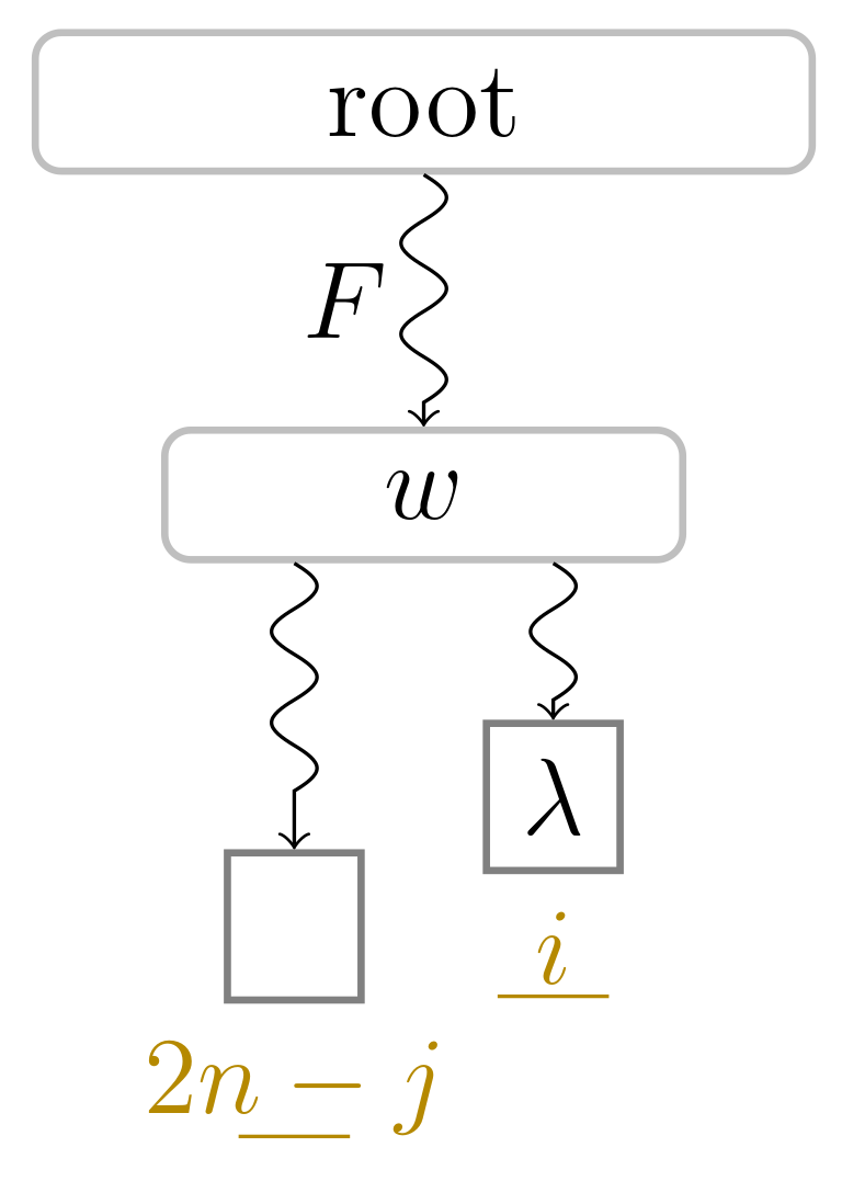
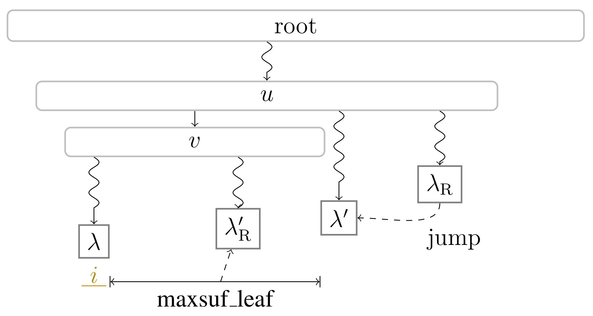
In the following, we describe our factorization algorithm working with ST . This algorithm performs traversals on paths connecting leaves with the root, during which it marks certain nodes. One kind of these marked nodes are phrase leaves: A phrase leaf is a leaf whose suffix number is the starting position of a factor. We say that a phrase leaf λ corresponds to a factor F if the suffix number of is the starting position of F. We call all other leaves non-phrase leaves. Another kind are witnesses, a notion borrowed from [21] ([Section 3]): Witnesses are nodes that create a connection between referencing factors and their referred positions. We formally define them as follows: given λ is the phrase leaf corresponding to a referencing factor F, the witness w of F is the LCA of λ and a leaf with suffix number 2 n j (with j [ 1 . . n 1 ] ) such that T [ j str _ depth ( w ) + 1 . . j ] R is the longest substring in T [ 1 . . sufnum ( λ ) 1 ] R that is a prefix of T [ sufnum ( λ ) . . ] . The smallest such j is the referred position of λ , which is needed for the coding in Section 3.1. See Figure 2 for a sketch of the setting. In what follows, we show that the witness of a referencing factor F is the node whose string label is F. Generally speaking, for each substring S of T, there is always a node whose string label has S as a prefix, but there maybe no node whose string label is precisely S. This is in particular the case for the non-overlapping LZSS factorization [22] ([Section 3.1]). Here, we can make use of the fact that the suffix number 2 n j for a referred position j is always larger than the length of T, which we want to factorize:
Lemma 1.
The witness of each referencing factor exists and is well-defined.
Proof. 
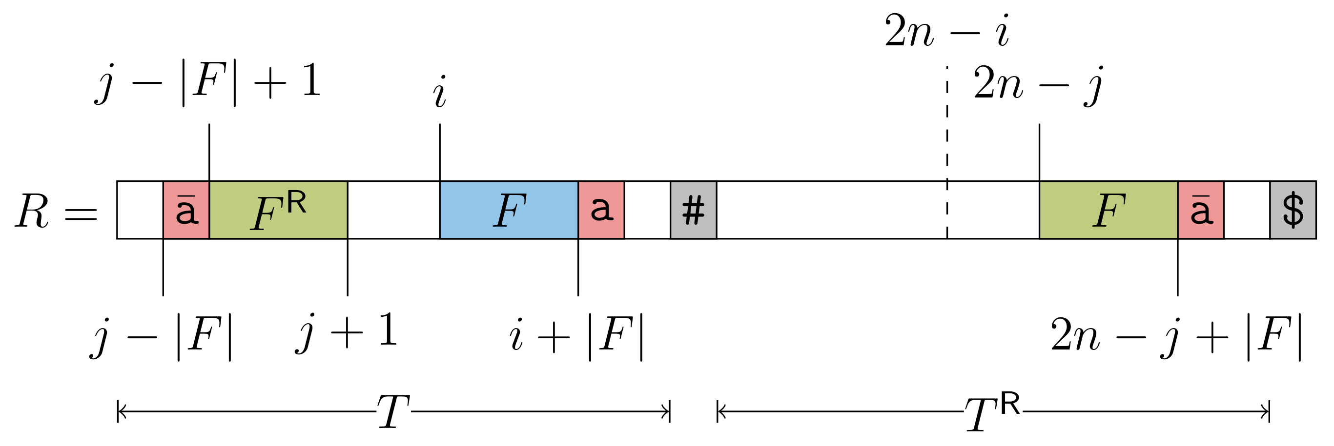
To show that each referencing factor is indeed the string label of an ST node, we review the definition of right-maximal repeats: A right-maximal repeat is a substring of R having at least two occurrences R [ i 1 . . i 1 + 1 ] and R [ i 2 . . i 2 + 1 ] with R [ i 1 + ] R [ i 2 + ] . A right-maximal repeat is the string label of an ST node since this node has at least two children; those two children are connected by edges whose labels start with R [ i 1 + ] and R [ i 2 + ] , respectively. It is therefore sufficient to show that each factor F is a right-maximal repeat. Given j is the referred position of F = T [ i . . i + | F | 1 ] , F = T [ j | F | + 1 . . j ] R = R [ 2 n j . . 2 n j + | F | 1 ] . If j = | F | , then T [ i + | F | ] R [ 2 n j + | F | ] = $ , and thus F is a right-maximal repeat. For the other case that j | F | + 1 , assume that F is not a right-maximal repeat. Then T [ i + | F | ] = R [ 2 n j + | F | ] = T [ j | F | ] . However, this means that F is not the longest reversed factor being a prefix of T [ i . . ] , a contradiction. We visualized the situation in Figure 3. □
Consequently, the referred position of a factor F x = T [ i . . i + 1 ] is the smallest text position j in T with j i 1 and one of the two equivalent conditions hold:
  • T [ j + 1 . . j ] R = T [ i . . i + 1 ] ; or
  • R [ i . . ] and R [ 2 n j . . ] have the longest common prefix of length .

3.2.1. Overview

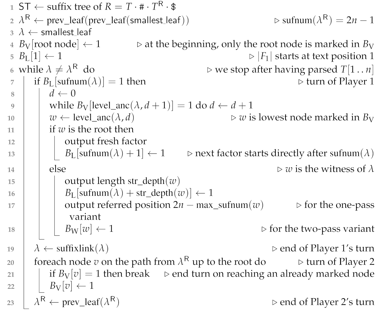
We explain our factorization algorithm in terms of a cooperative game with two players (We use this notation only for didactic purposes; the terminology must not be confused with game theory. Here, the notion of player is basically a subroutine of the algorithm having private and shared variables.), whose pseudo code we sketched in Algorithm 1. Player 1 and Player 2 are allowed to access the leaves with suffix numbers in the ranges [ 1 . . n ] and [ n . . 2 n 1 ] , respectively. Player 1 (resp. Player 2) starts at the leaf with the smallest (resp. largest) suffix number, and is allowed to access the leaf with the subsequently next (resp. previous) suffix number via suffixlink (resp. prev _ leaf ). Hence, Player 1 simulates a linear forward scan in the text T, while Player 2 simulates a linear backward scan in T R . Both players take turns at accessing leaves at the same pace. To be more precise, in the i-th turn, Player 1 processes the leaf with suffix number i, whereas Player 2 processes the leaf with suffix number 2 n i . In one turn, a player accesses a leaf λ and maybe performs a traversal on the path connecting the root with λ . For such a traversal, we use level ancestor queries to traverse each node on the path in constant time. Whenever Player 2 accesses the leaf with suffix number n (shared among both players), the game ends; at that time both players access the same leaf (cf. Line 6 in Algorithm 1). In the following, we call this game a pass (with the meaning that we pass all relevant text positions). Depending on the allowed working space, our algorithm consists of one or two passes (cf. Section 3.3). The goal of Player 2 is to keep track of all nodes she visits. Player 2 does this by maintaining a bit vector B V of length 4 n such that B V [ v ] stores whether a node v has already been visited by Player 2, where we represent a node v by its pre-order number when using it as an index of a bit vector. To keep things simple, we initially mark the root node in B V at the start of each pass. By doing so, after the i-th turn of Player 2 we can read any substring of T [ 1 . . i ] R by a top-down traversal from the suffix tree root, only visiting nodes marked in B V . This is because of the invariant that the set of nodes marked in B V is upper-closed, i.e., if a node v is marked in B V , then all its ancestors are marked in B V as well.
The goal of Player 1 is to find the phrase leaves and the witnesses. For that, she maintains two bit vectors B L and B W of length n and 4 n , respectively, whose entries are marked similarly to B V by using the suffix numbers ( [ 1 . . n ] ) of the leaves accessed by Player 1 and preorder numbers of the internal nodes. We initially mark smallest _ leaf in B L since text position 1 is always the starting position of the fresh factor F 1 . By doing so, after the i-th turn of Player 1 we know the ending positions of those factors contained in T [ 1 . . i ] , which are marked in B L . To sum up, after the i-th turn of both players we know the computed factors starting at text positions up to i thanks to Player 1, and can find the factor lengths thanks to Player 2, which we explain in detail in Section 3.2.2. There, we will show that the actions of Player 2 allow Player 1 to determine the starting position of the next factor. For that, she computes the string depth of the lowest ancestor marked in B V of the previously visited phrase leaf. See Appendix A.
As a side note: since we are only interested in the factorization of T [ 1 . . n 1 ] (omitting the appended # at position n), we do not need Player 1 to declare the leaf with suffix number n a phrase leaf. We also terminate the algorithm when both players meet at position n without checking whether we have found a new factor starting at position n.
Algorithm 1: Algorithm of Section 3.2.2 computing the non-overlapping reversed LZ factorization. The function max _ sufnum is described in Section 3.3.
Algorithms 14 00161 i001

3.2.2. One-Pass Algorithm in Detail

In detail, a pass works as follows: at the start, Player 1 and Player 2 select smallest _ leaf and prev _ leaf ( prev _ leaf ( smallest _ leaf ) ) , i.e., the leaves with suffix numbers 1 and 2 n 1 , respectively. Now the players take action in alternating turns, starting with Player 1. Nevertheless, we first explain the actions of Player 2, since Player 2 acts independently of Player 1, while Player 1’s actions depend on Player 2.
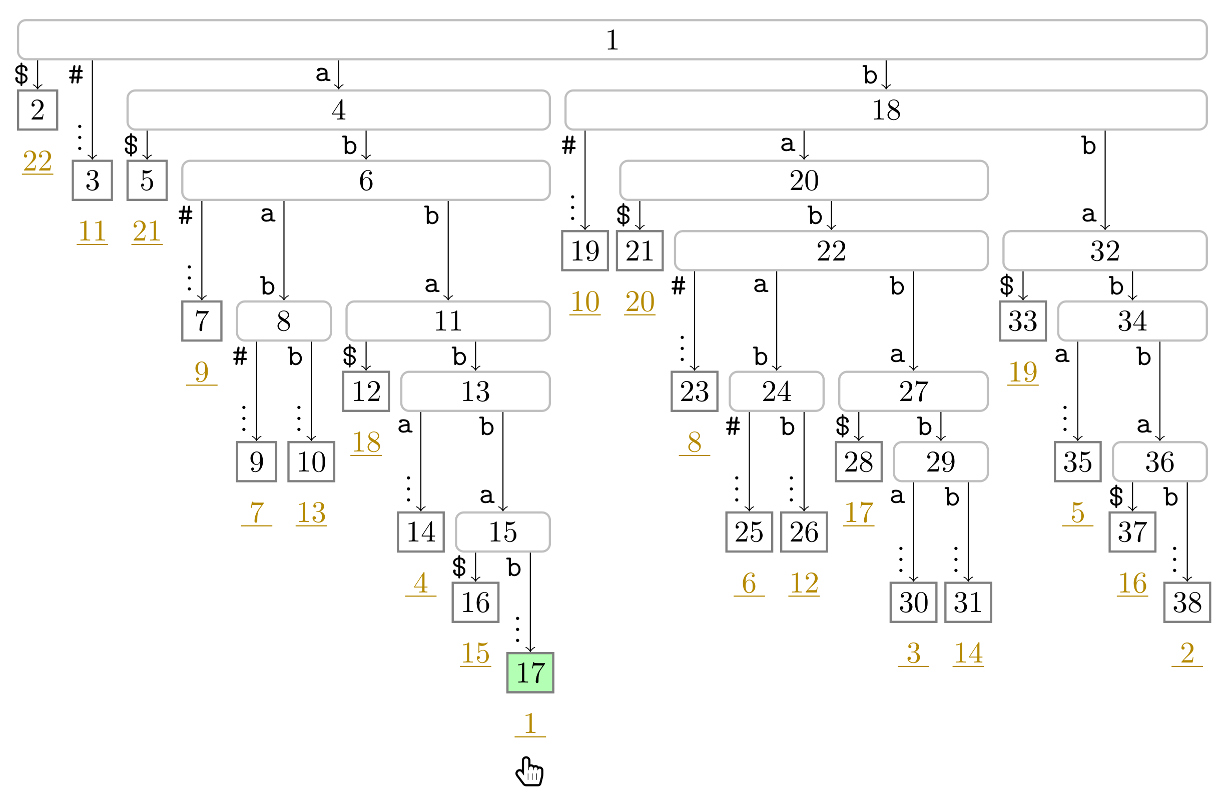
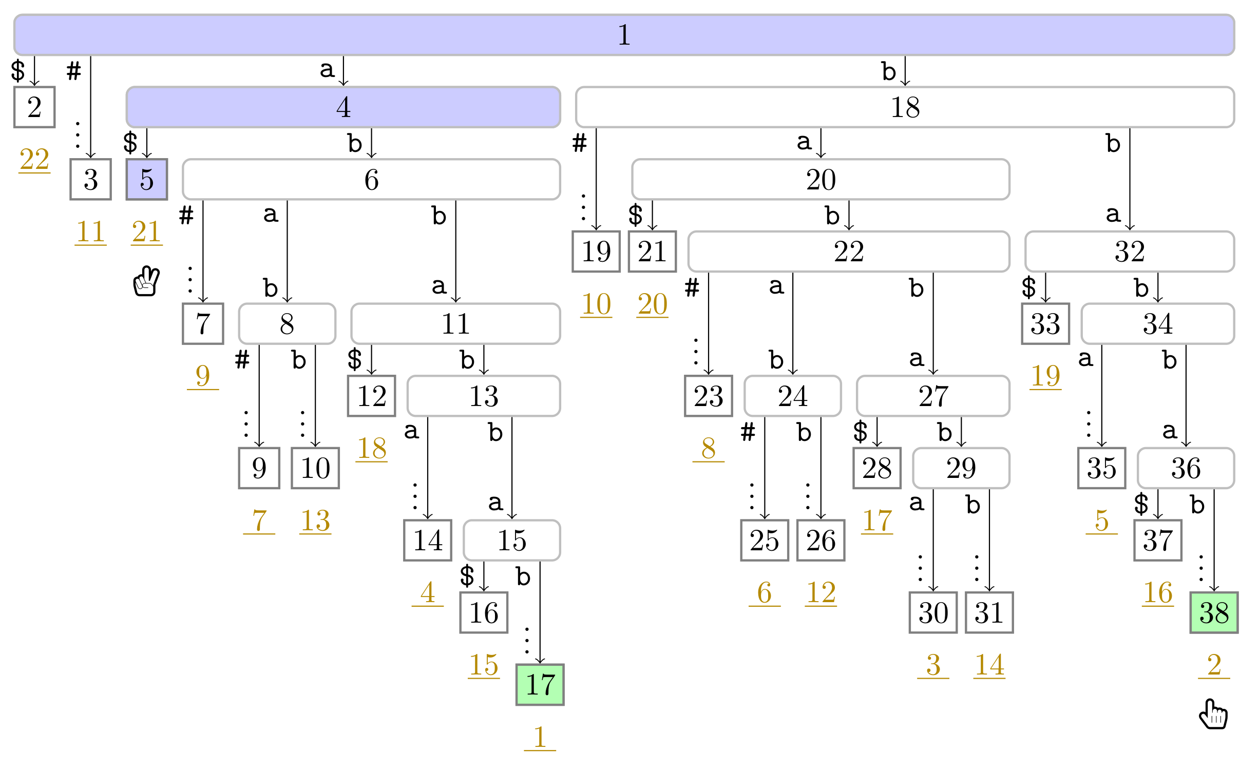
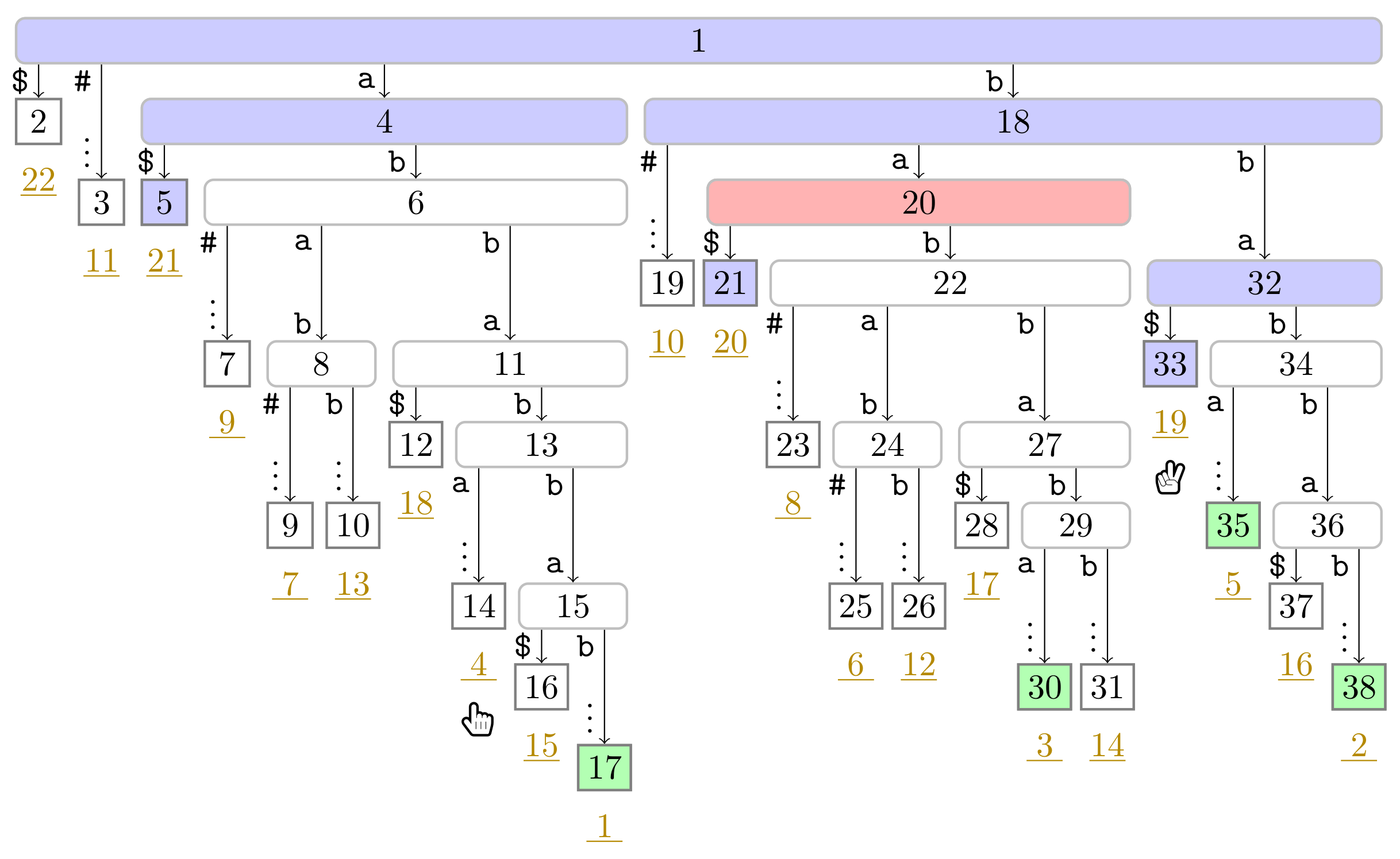
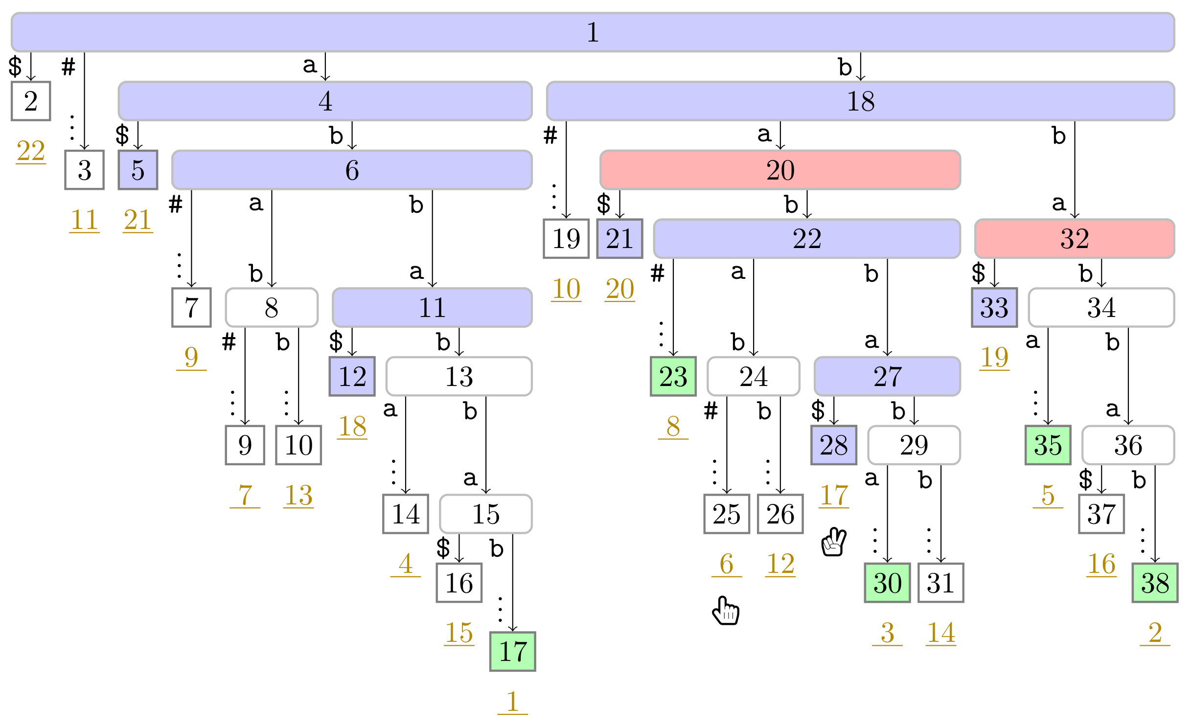
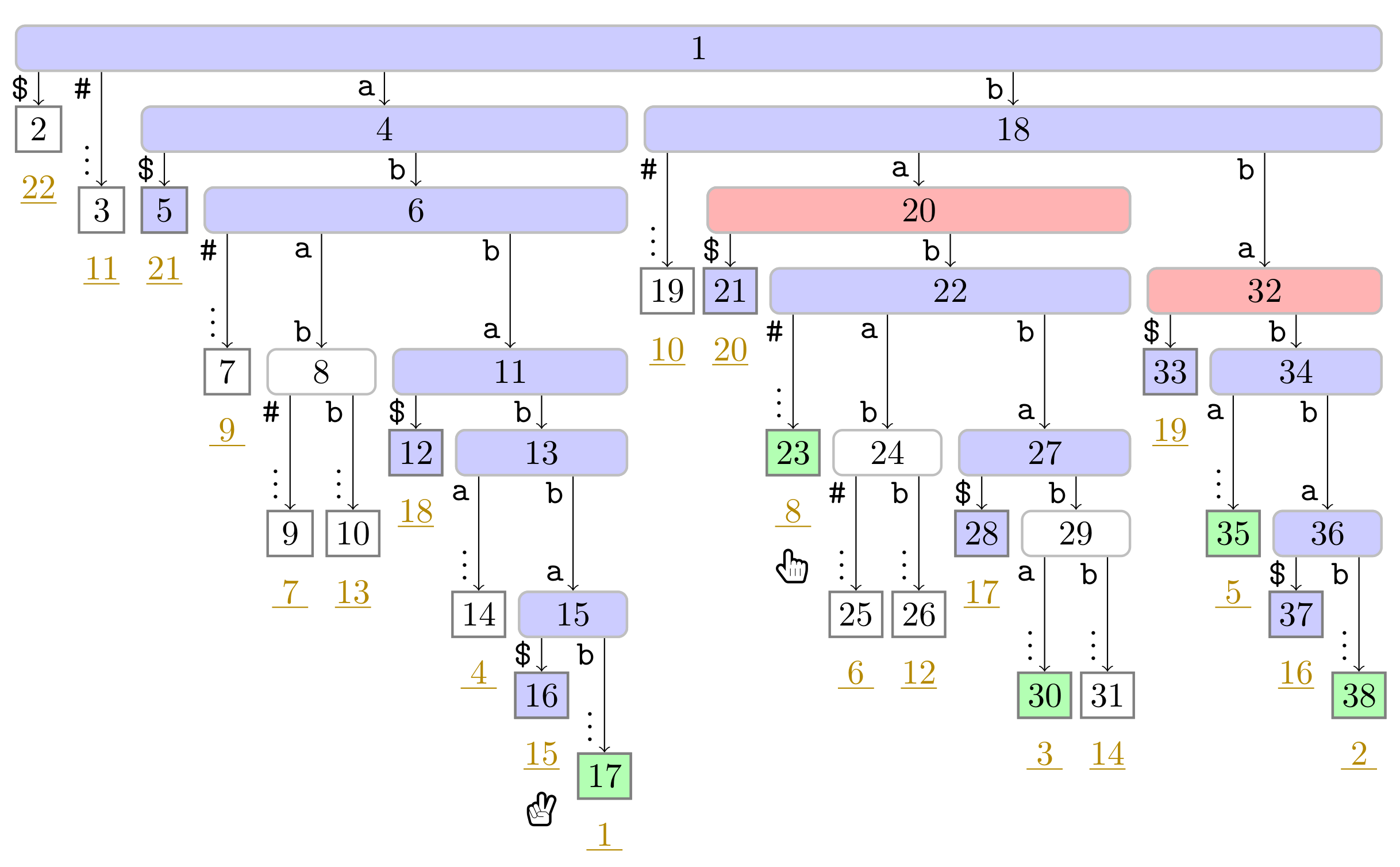
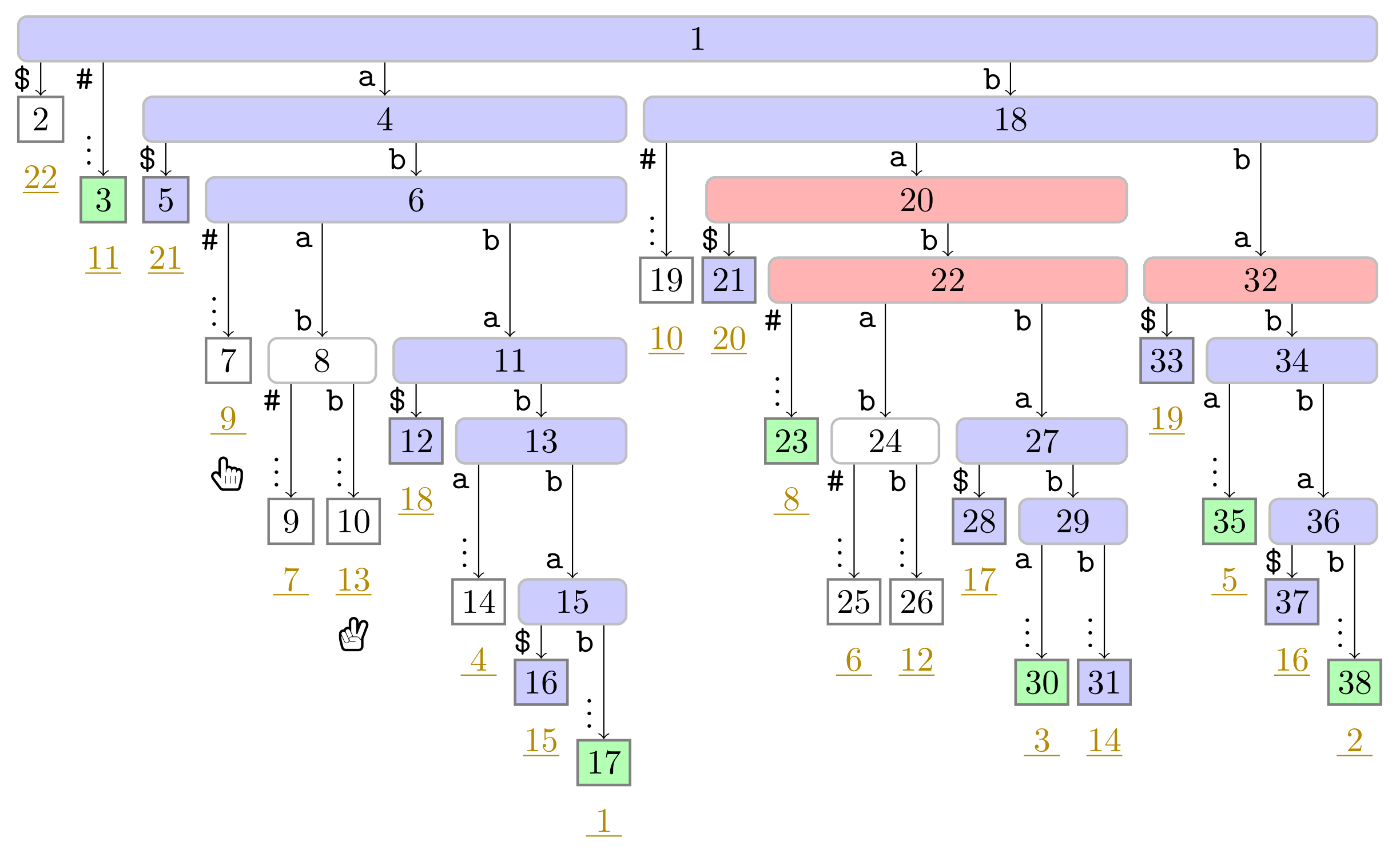
Suppose that Player 2 is at a leaf λ R (cf. Line 20 of Algorithm 1). Player 2 traverses the path from λ R to the root upwards and marks all visited nodes in B V until arriving at a node v already marked in B V (such a node exists since we mark the root in B V at the beginning of a pass.). When reaching the marked node v, we end the turn of Player 2, and move Player 2 to prev _ leaf ( λ R ) at Line 23 (and terminate the whole pass in Line 6 when this leaf has suffix number n). The foreach loop (Line 20) of the algorithm can be more verbosely expressed with a loop iterating over all depth offsets d in increasing order while computing v level _ anc ( λ R , d ) until either reaching the root or a node marked in B V . Subsequently, the turn of Player 1 starts (cf. Line 7). We depict the state after the first turn of Player 2 in Figure 4.
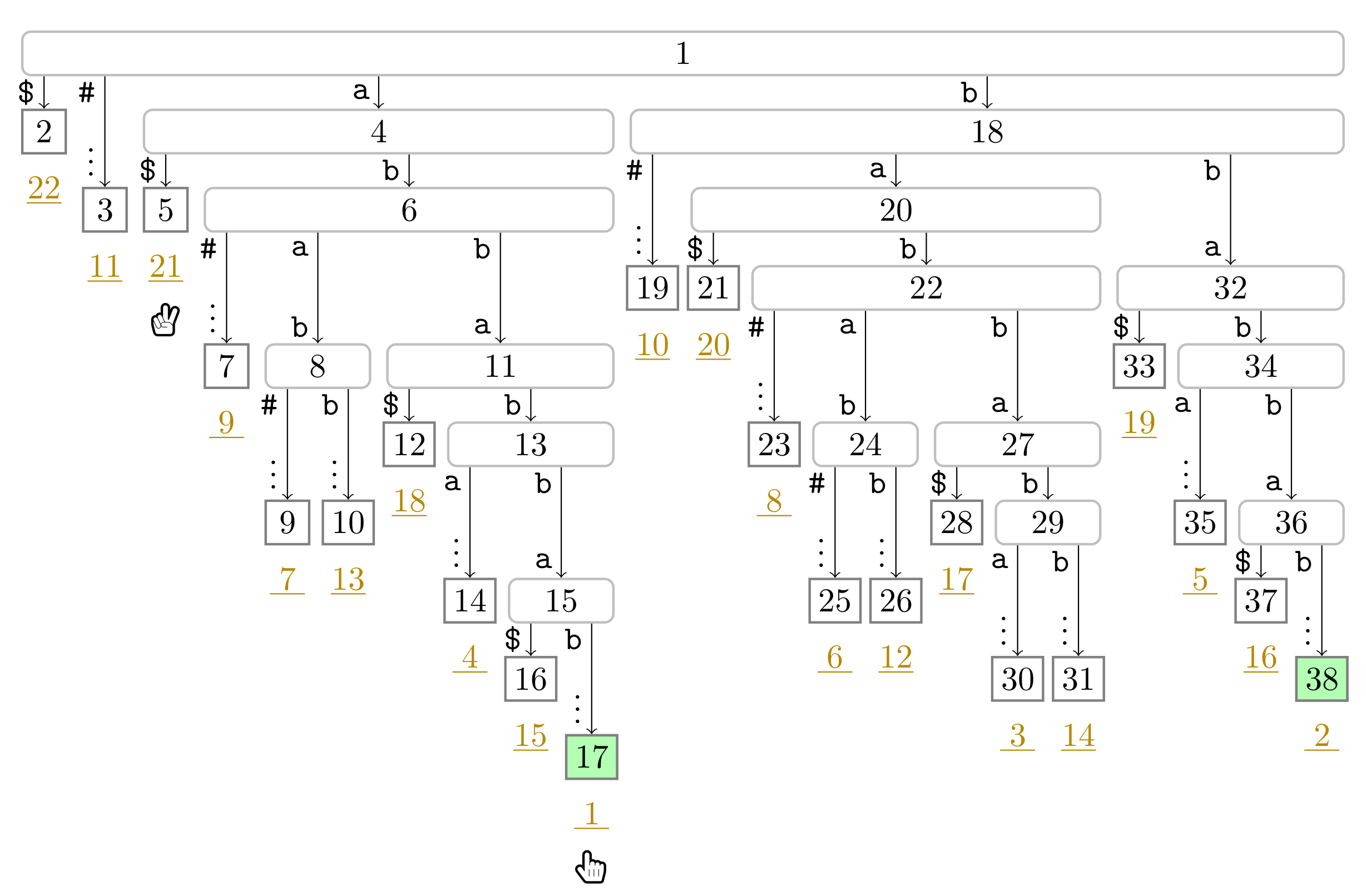
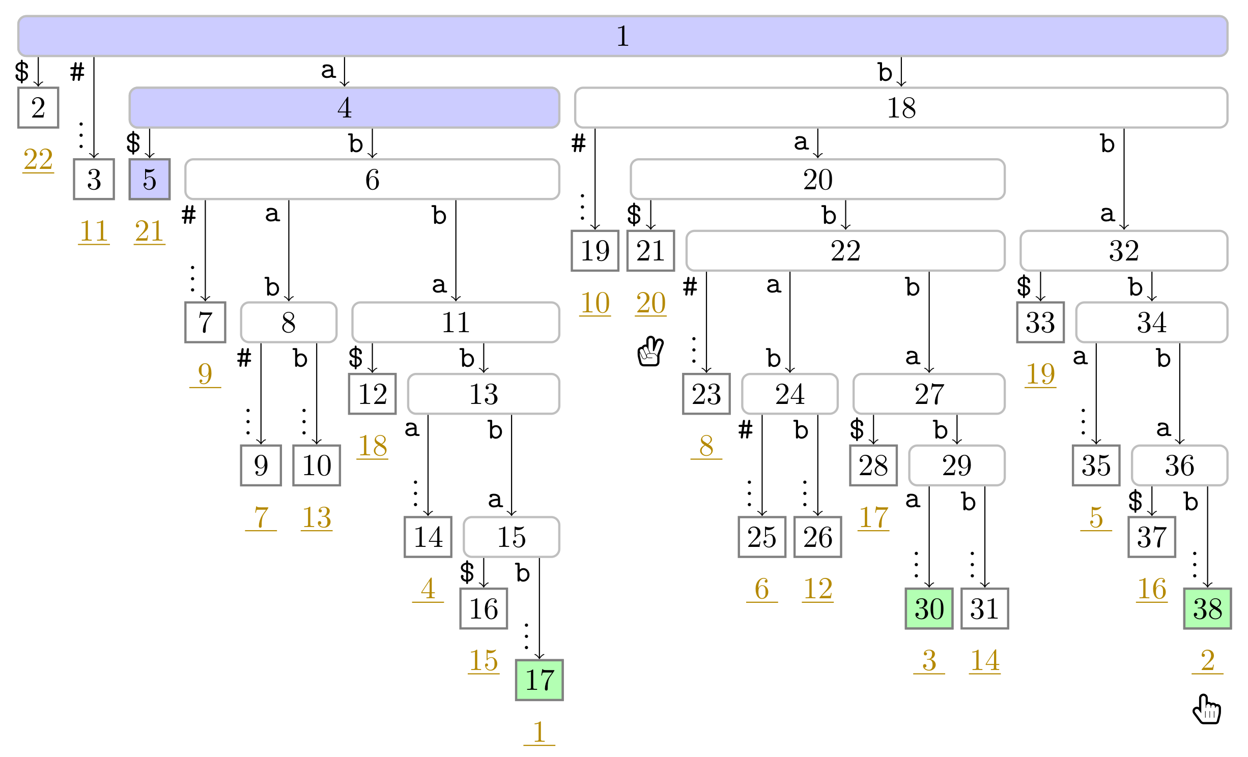
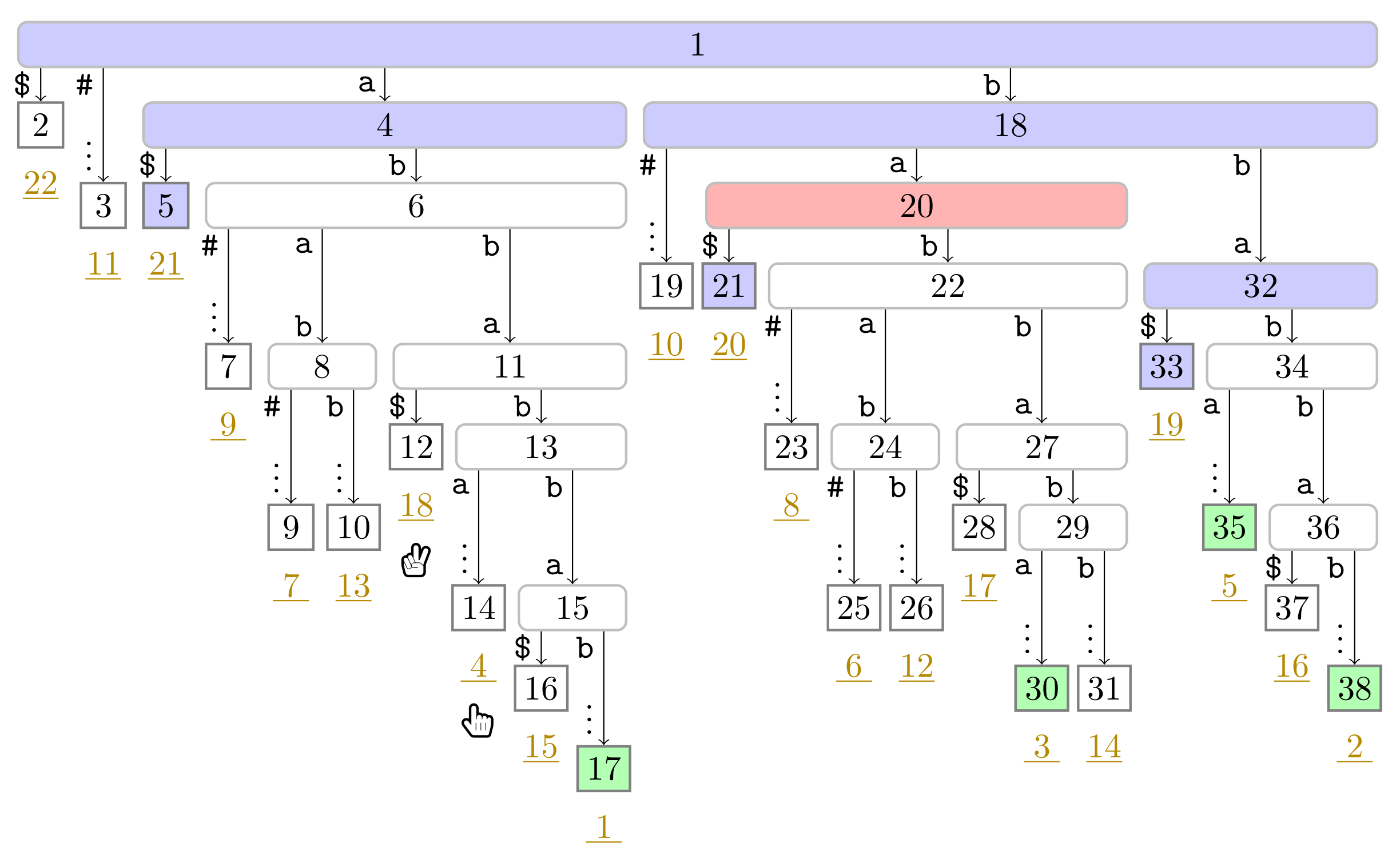
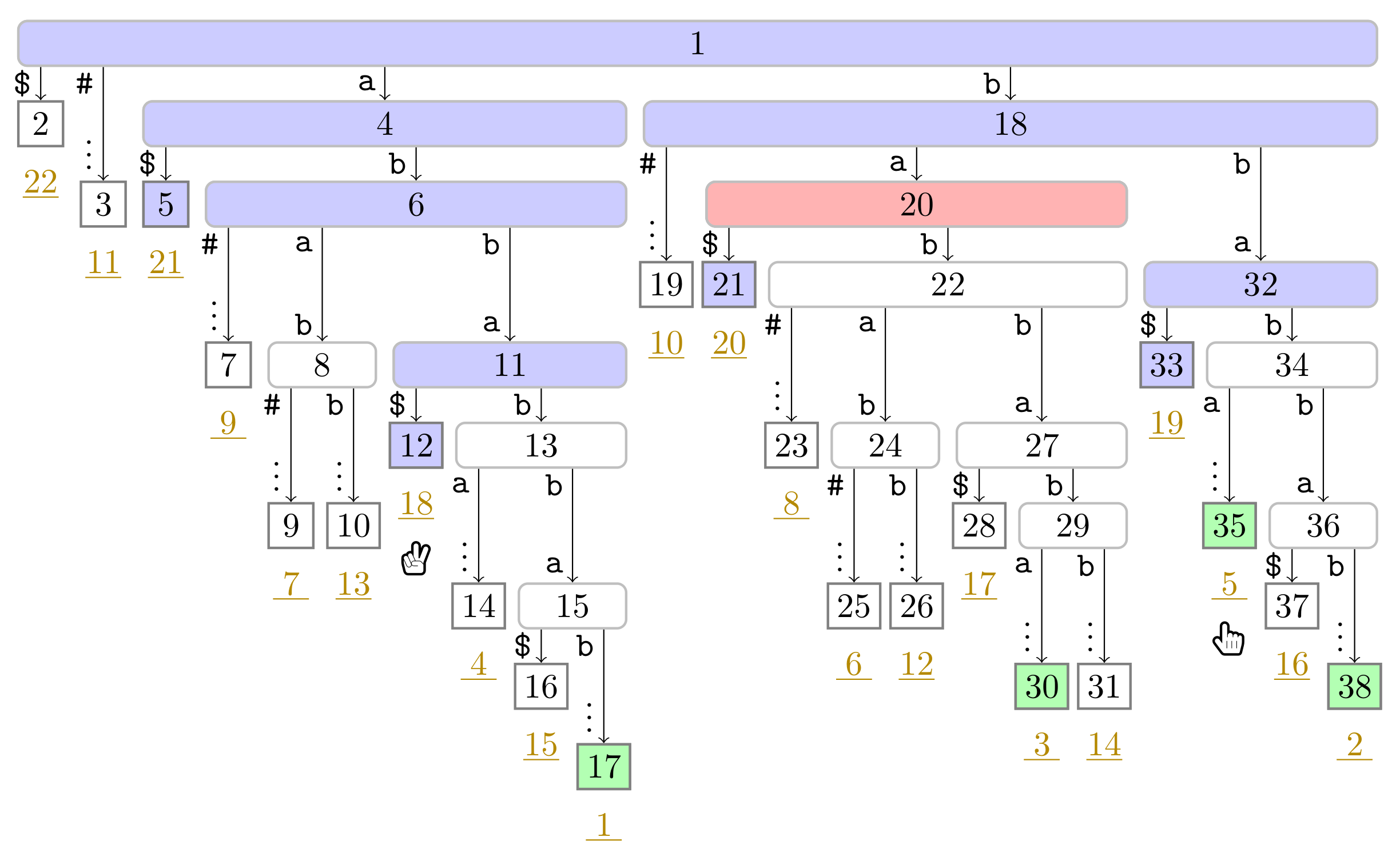
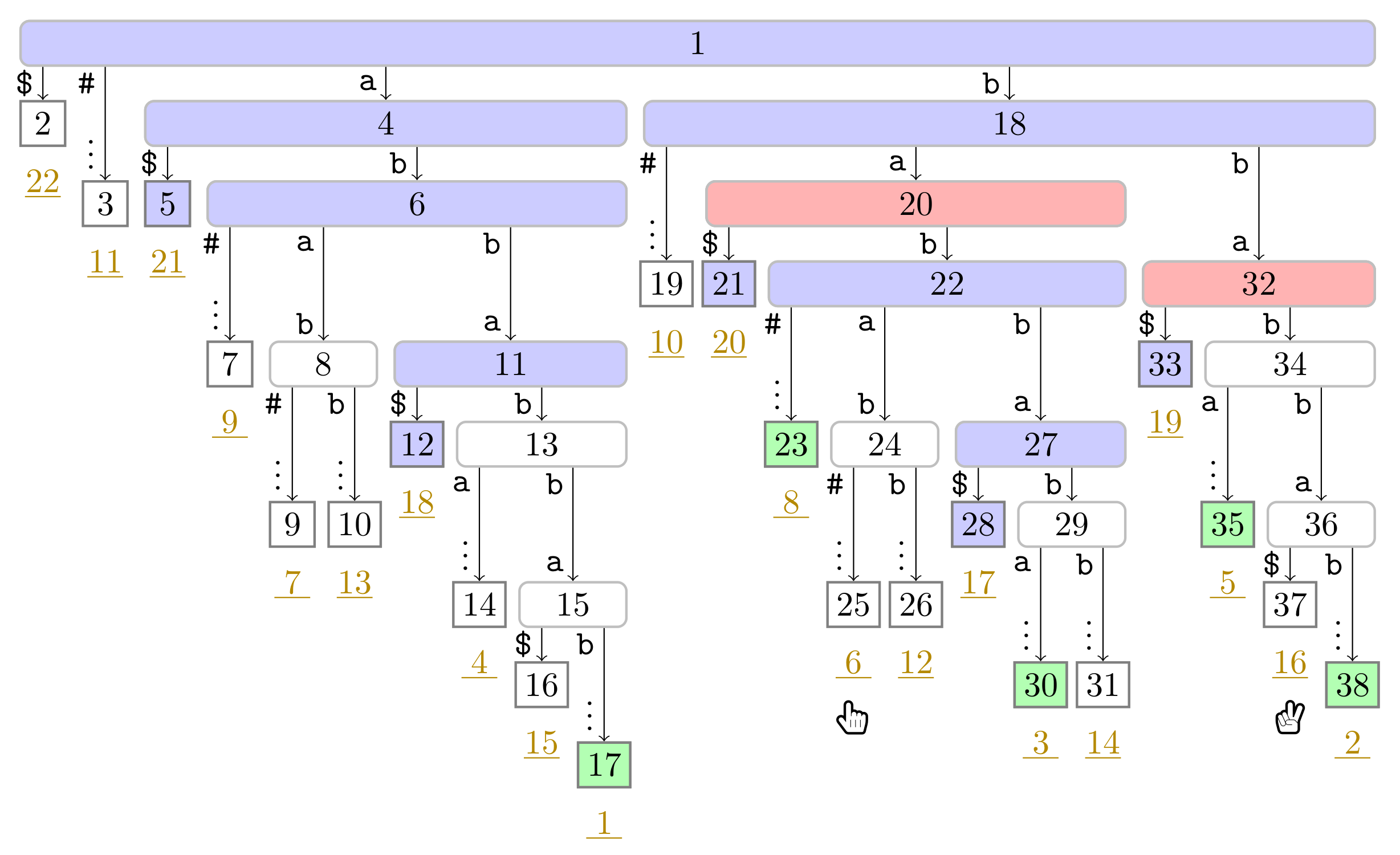
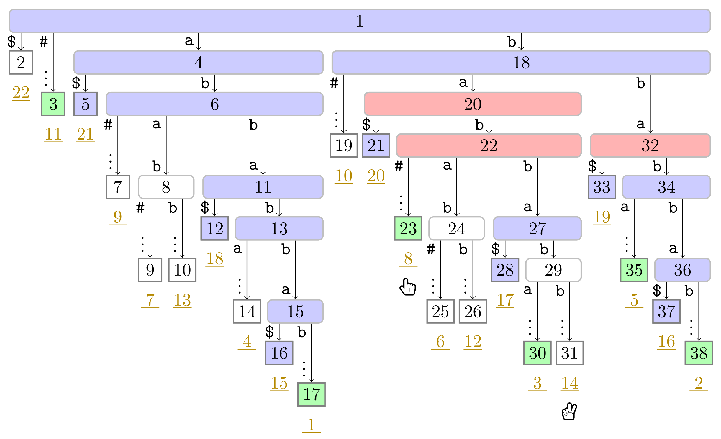
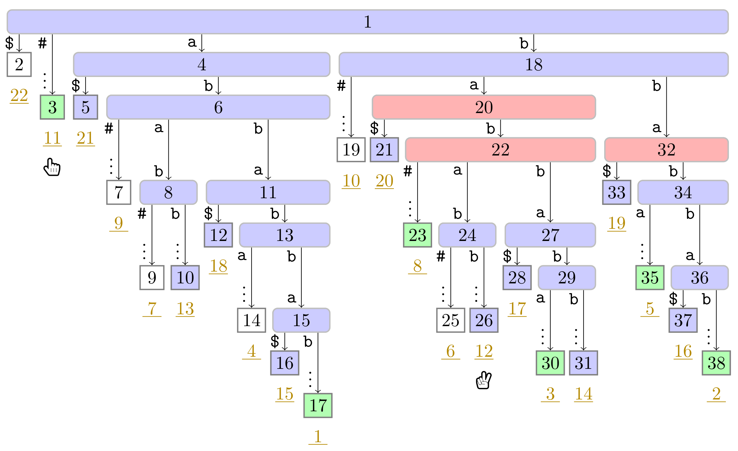
If Player 1 is at a non-phrase leaf λ , we skip the turn of Player 1, move Player 1 to suffixlink ( λ ) at Line 19, and let Player 2 take action. Now suppose that Player 1 is at a phrase leaf λ corresponding to a factor F. Then we traverse the path from the root to λ downwards to find the lowest ancestor w of λ marked in B V . If w is the root node, then F is a fresh factor (cf. Line 11), and we know that the next factor starts immediately after F (cf. Line 13). Consequently, the leaf suffixlink ( λ ) is a phrase leaf. Otherwise, w is the witness of λ , and str _ depth ( w ) = | F | (cf. Line 14). Hence, sufnum ( λ ) + str _ depth ( w ) is the suffix number of the phrase leaf λ ˜ that Player 1 will subsequently access. We therefore mark w and sufnum ( λ ˜ ) = sufnum ( λ ) + str _ depth ( w ) in B W and in B L , respectively (cf. Lines 16 and 18). We depict the fifth turn of our running example in Figure 5, during which Player 1 marks a witness node. Finally, we end the turn of Player 1, move Player 1 to suffixlink ( λ ) at Line 19, and let Player 2 take action.
Correctness. When Player 1 accesses the leaf λ with suffix number i, Player 2 has processed all leaves with suffix numbers [ 2 n i + 1 . . 2 n 1 ] . Due to the leaf-to-root traversals of Player 2, each node marked in B V has a leaf with a suffix number in [ 2 n i + 1 . . 2 n 1 ] in its subtree. In particular, a node w is marked in B V if and only if the string label of w is a substring of R [ 2 n i + 1 . . 2 n 1 ] . Because R [ 2 n i + 1 . . 2 n 1 ] R = T [ 1 . . i 1 ] , the longest prefix of T [ i . . ] having a reversed occurrence in T [ 1 . . i 1 ] is therefore one of the string labels of the nodes marked in B V . In particular, we search the longest string label among those nodes, which we obtain with the lowest ancestor of λ marked in B V .

3.2.3. Time Complexity

First, let us agree on that we never compute the suffix number of a leaf since this is a costly operation for CST (cf. Table 3). Although we need the suffix numbers at multiple occasions, we can infer them if each player maintains a counter for the suffix number of the currently visited leaf. A counter is initialized with 1 (resp. 2 n 1 ) and becomes incremented (resp. decremented) by one when moving to the succeeding (resp. preceding) leaf in suffix number order. This works since both players traverse the leaves linearly in the order of the suffix numbers (either in ascending or descending order).
Player 2 visits n leaves, and visits only unvisited nodes during a leaf-to-root traversal. Hence, Player 2’s actions take O ( n ) overall time.
Player 1 also visits n leaves. Since Player 1 has no business with the non-phrase leaves, we only need to analyze the time spent by Player 1 for a phrase leaf corresponding to a factor F: If F is fresh, then the root-to-leaf traversal ends prematurely at the root, and hence we can determine in constant time whether F is fresh or not. If F is referencing, we descend from the root to the lowest ancestor w marked in B V , and compute str _ depth ( w ) to determine the suffix number of the next phrase leaf (cf. Line 15 of Algorithm 1). Since depth ( w ) str _ depth ( w ) , we visit at most | F | + 1 nodes before reaching w. Computing str _ depth ( w ) takes O ( 1 / ϵ ) time for the SST, and O ( | F | ) time for the CST. This seems costly, but we compute str _ depth ( w ) for each factor only once. Since the sum of all factor lengths is n, we spend O ( n + z / ϵ ) time or O ( n ) time for computing all factor lengths when using the SST or the CST, respectively. We finally obtain the time bounds stated in Theorem 1 for computing the factorization.

3.3. Determining the Referred Position

Up to now, we can determine the reversed-LZ factors F 1 F z = T with B L marking the starting position of each factor with a one. Yet, we have not the referred positions necessary for the coding of the factors (cf. Section 3.1). To obtain them, we have two options: The first option is easier but comes with the requirement for a support data structure on ST for the operation
max _ sufnum ( v )
returning the maximum among all suffix numbers of the leaves in the subtree rooted in v.
We can build such a support data structure in O ( ϵ 1 n ) time (resp. O ( ϵ 1 n log σ ϵ n ) time) using O ( n ) bits to support max _ sufnum in O ( ϵ 1 ) time (resp. O ( ϵ 1 log σ ϵ n ) time) for the SST (resp. CST); see [22] ([Section 3.3]). Being able to query max _ sufnum , we can directly compute the referred position of a factor F when discovering its witness w during a turn of Player 1 by max _ sufnum ( w ) . max _ sufnum ( w ) gives us the suffix number of a leaf that has already been accessed by Player 2 since Player 2 accesses the leaves in descending order with respect to the suffix numbers, and w must have already been accessed by Player 2 during a leaf-to-root traversal (otherwise w would not have been marked in B V ). Since R [ max _ sufnum ( w ) . . max _ sufnum ( w ) + str _ depth ( w ) 1 ] = F R , the referred position of F is 2 n max _ sufnum ( w ) . Consequently, we can compute the coding of the factors during a single pass (cf. Line 17 of Algorithm 1), and are done when the pass finishes.
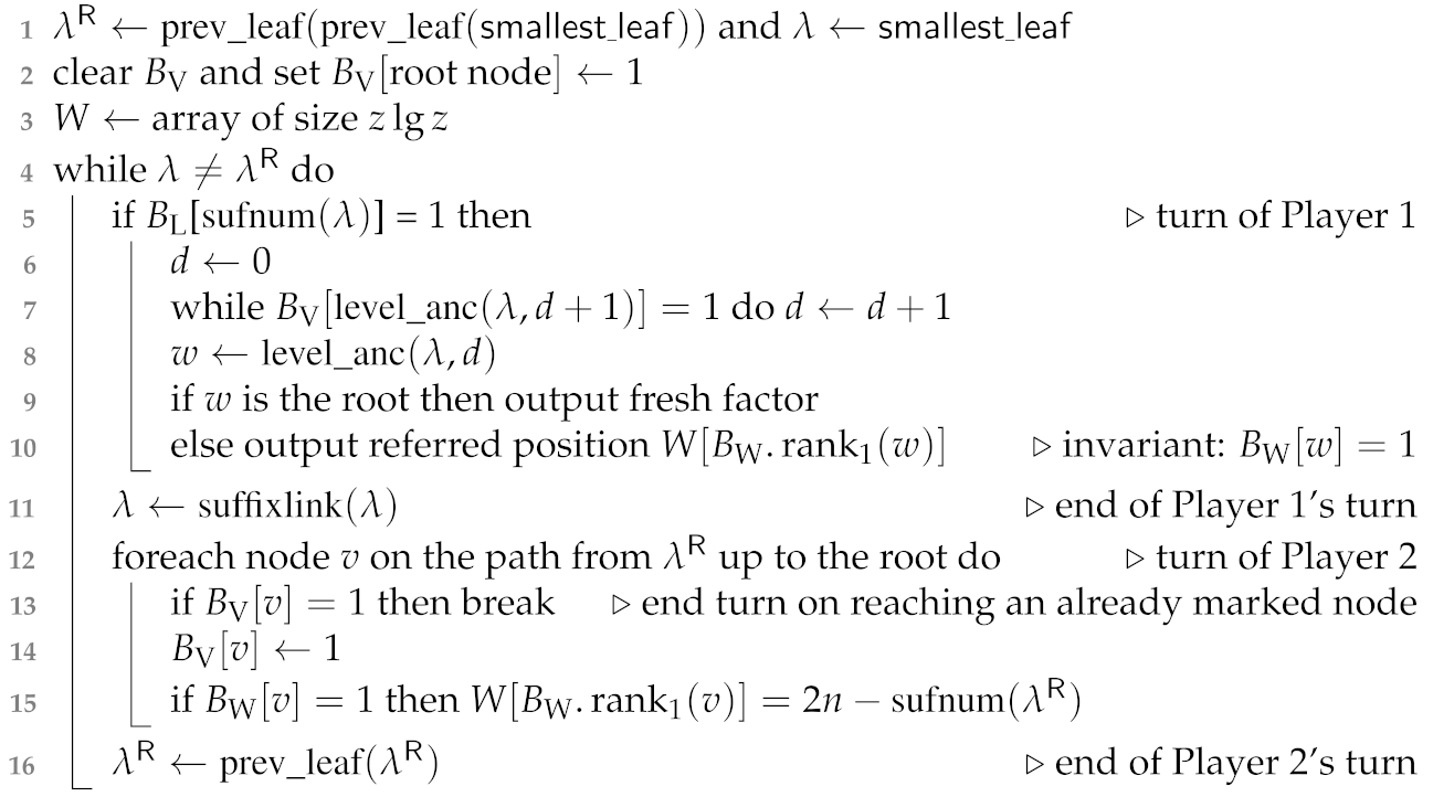
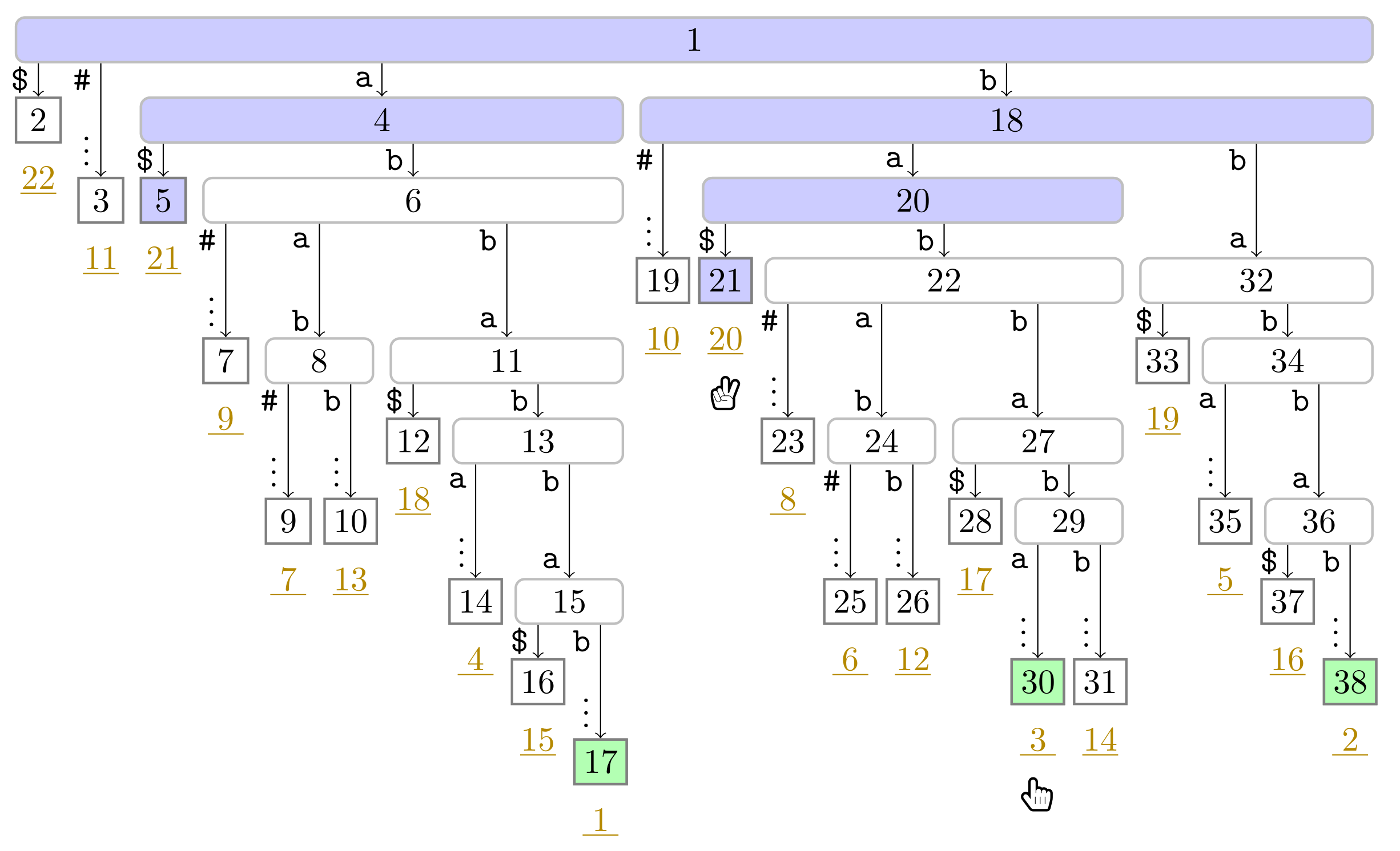
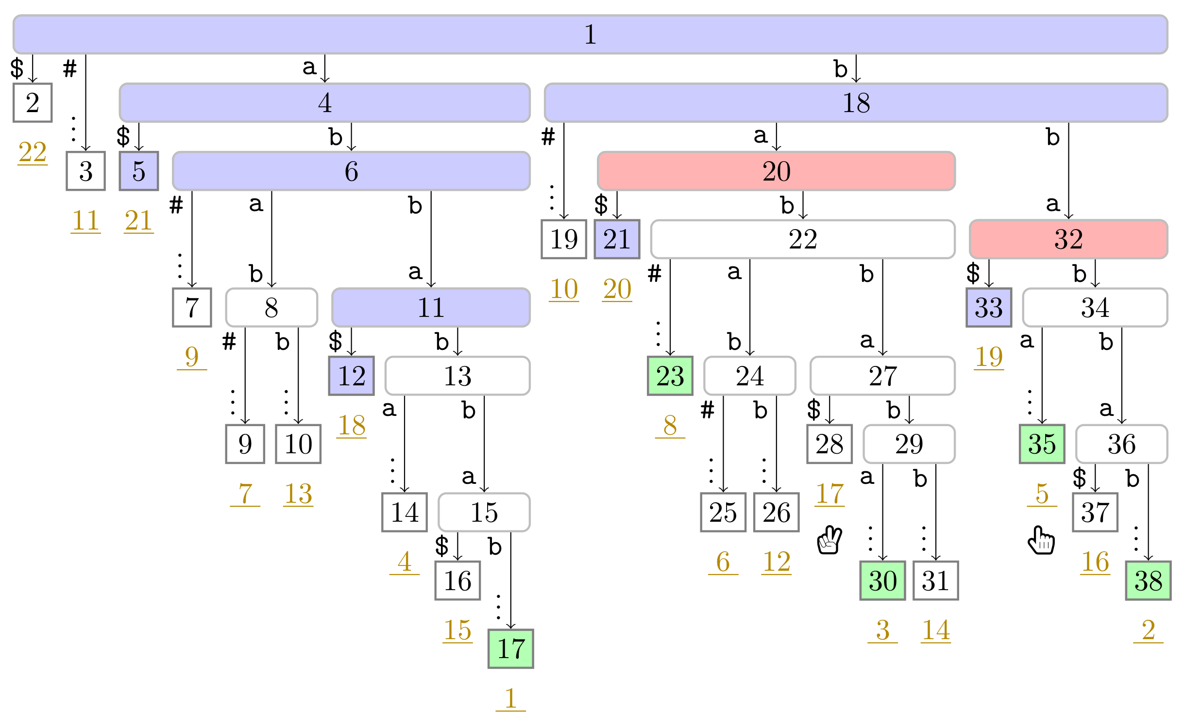
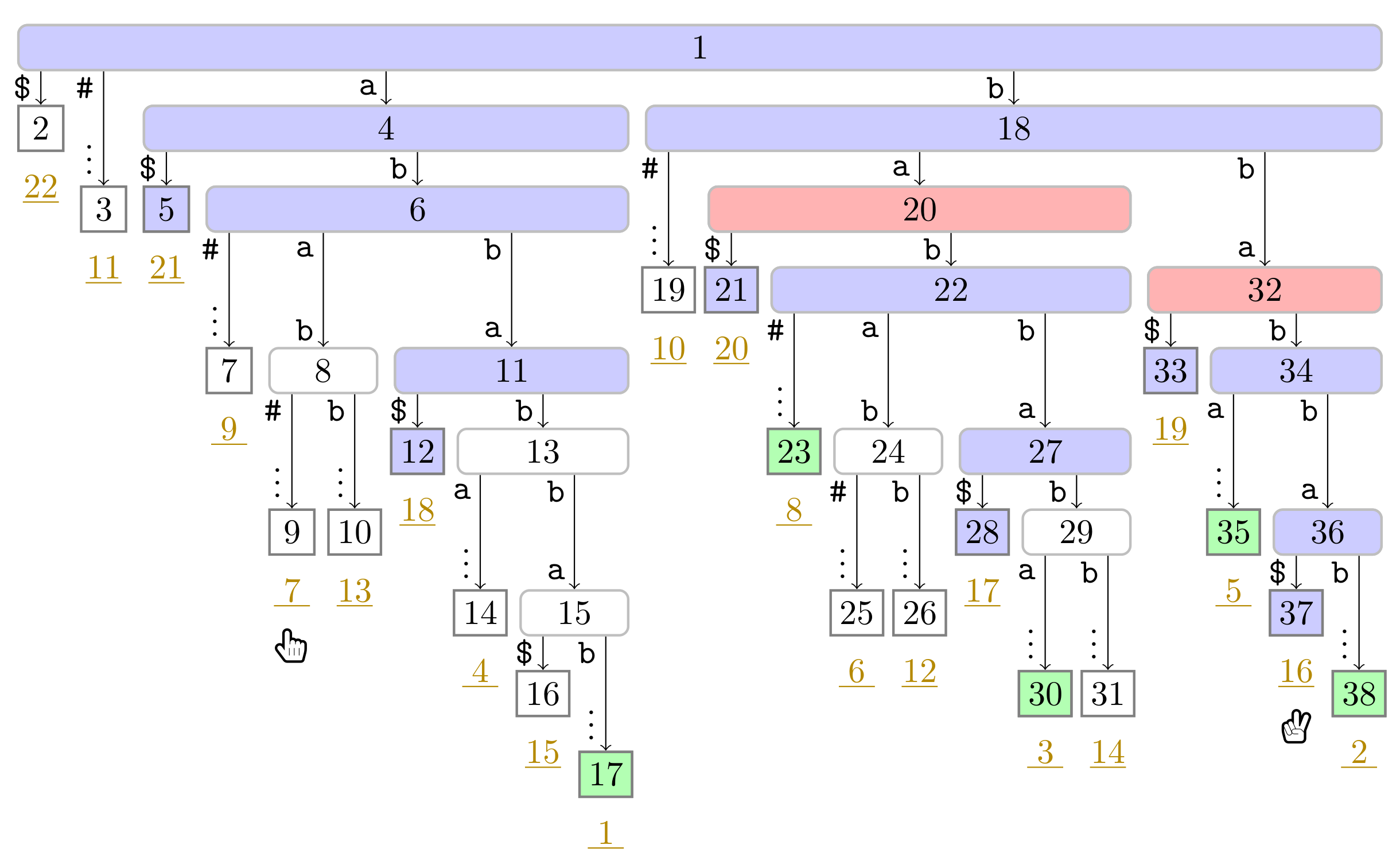
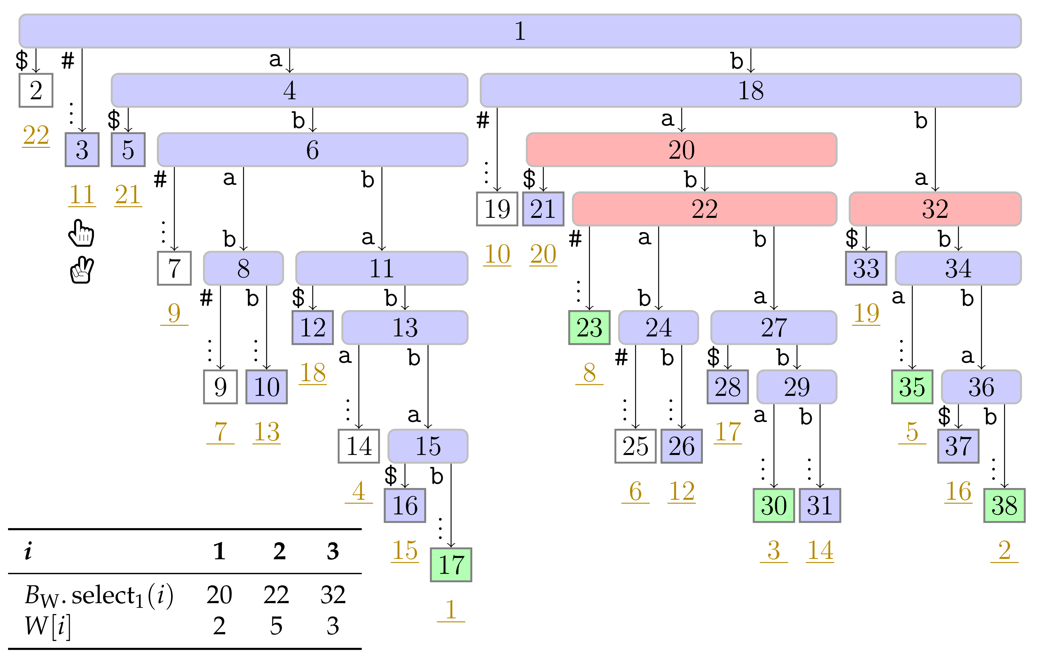
The second option does not need to compute max _ sufnum and retains the linear time bound when using CST. Here, the idea is to run an additional pass, whose pseudo code is given in Algorithm 2. For this additional pass, we do the following preparations: Let z W be the number of witnesses, which is at most z since there can be multiple factors having the same witness. We keep B L and B W marking the phrase leaves and the witnesses, respectively. However, we clear B V such that Player 2 has again the job to log her visited nodes in B V . We augment B W with a rank-support such that we can enumerate the witnesses with ranks from 1 to at most z W , which we call the witness rank. We additionally create an array W of z W lg n bits. We want W [ B W . rank 1 ( w ) ] to store the referred position 2 n max _ sufnum ( w ) [ 1 . . n 1 ] for each witness w such that we can read the respective referred position from W when Player 1 accesses w. We assign the task for maintaining W to Player 2. Player 2 can handle this task by taking additional action when visiting a witness (i.e., a node marked in B W ) during a leaf-to-root traversal: When visiting a witness node w with witness rank i from a leaf λ , we write W [ i ] 2 n sufnum ( λ ) if w is not yet marked in B V (cf. Line 15 in Algorithm 2). Like before, Player 2 terminates her turn whenever she visits an already visited node. The actions of Player 1 differ in that she no longer needs to compute B L and B W : When Player 1 visits a phrase leaf λ , she locates the lowest ancestor w of λ marked in B V , which has to be marked in B W , too (as a side note: storing the depth of the witness of each phrase leaf in a list, sorted by the suffix numbers of these leaves, helps us to directly jump to the respective witness in constant time. We can encode this list as a bit vector of length O ( n ) by storing each depth in unary coding (cf. [22] ([Section 3.4])). Nevertheless, we can afford the root-to-witness traversals of Player 1 since we visit at most x = 1 z | F x | = n nodes in total.). With the rank-support on B W , we can compute w’s witness rank i, and obtain the referred position of λ with W [ i ] (cf. Line 10 of Algorithm 2). We show the final state after the first pass in Figure 6, together with W computed in the second pass.
Overall, the time complexity is O ( ϵ 1 n ) time when working with either the SST or the CST. We use o ( n ) additional bits of space for the rank-support of B W , but costly z W lg n bits for the array W. However, we can bound z W by O ( n lg σ / lg n ) since z W is the number of distinct reversed LZ factors, and by an enumeration argument [40] ([Thm. 2]), a text of length n can be partitioned into at most O ( n / log σ n ) distinct factors. Hence, we can store W in z W lg n = O ( n lg σ ) bits of space. With that, we finally obtain the working space bound of O ( ϵ 1 n lg σ ) bits for the CST solution as claimed in Theorem 1.
Algorithm 2: Determining the referred positions in a second pass described in Section 3.3.
Algorithms 14 00161 i002

4. Computing LPnrF

The longest previous non-overlapping reverse factor table LPnrF [ 1 . . n ] is an array such that LPnrF [ i ] is the length of the longest prefix of T [ i . . ] · # occurring as a substring of T [ 1 . . i 1 ] R . (Appending # at the end is not needed, but simplifies the analysis for T [ 1 . . n 1 ] · # having precisely n characters.) Having LPnrF , we can iteratively compute the reversed LZ factorization because F x = T [ k x . . k x + max ( 0 , LPnrF [ k x ] 1 ) ] with k x 1 + y = 1 x 1 | F y | for x [ 1 . . z ] .
The counterpart of LPnrF for the non-overlapping LZSS factorization is the longest previous non-overlapping factor table LPnF [ 1 . . n ] , which is defined similarly, but stores the maximal length of the longest common prefix (LCP) of T [ i . . ] with all substrings T [ j . . i 1 ] for j [ 1 . . i 1 ] . See Table 4 for a comparison. Analogously to [34] ([Corollary 5]) or [24] ([Definition 4]) for the longest previous factor table LPF [22,26] ([Lemma 1]) for LPnF , LPnrF holds the following property:
Lemma 2
([14] (Lemma 2)). LPnrF [ i 1 ] 1 LPnrF [ i ] n i for i [ 2 . . n ] .
Hence, we can encode LPnrF in 2 n bits by writing the differences LPnrF [ i ] LPnrF [ i 1 ] + 1 0 in unary, obtaining a bit sequence of (a) n ones for the n entries and (b) i = 2 n ( LPnrF [ i ] LPnrF [ i 1 ] + 1 ) n many zeros. We can decode this bit sequence by reading the differences linearly because we know that LPnrF [ 1 ] = 0 .

4.1. Adaptation of the Single-Pass Algorithm

Having an O ( n ) -bits representation of LPnrF gives us hope to find an algorithm computing LPnrF in a total workspace space of o ( n lg n ) bits. Indeed, we can adapt our algorithm devised for the reversed LZ factorization to compute LPnrF . For that, we just have to promote all leaves to phrase leaves such that the condition in Line 7 of Algorithm 1 is always true. Consequently, Player 1 performs a root-to-leaf traversal for finding the lowest node marked in B V of each leaf. By doing so, the time complexity becomes O ( n 2 ) , however, since we visit at most i = 1 n LPnrF [ i ] = O ( n 2 ) many nodes during the root-to-leaf traversals (there are strings like T = a a for which this sum becomes Θ ( n 2 ) ).
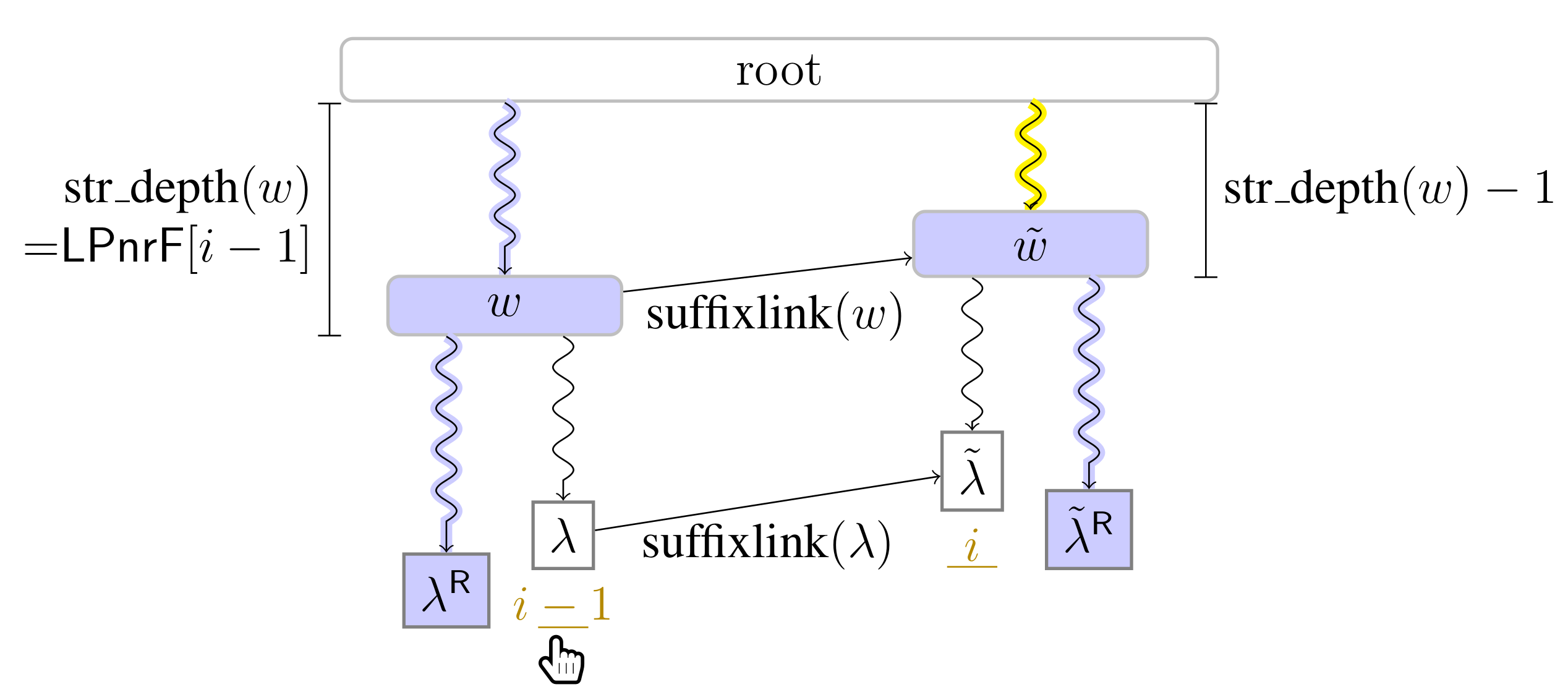
To lower this time bound, we follow the same strategy as in [22] ([Section 3.5]) or [34] ([Lemma 6]) using suffixlink and Lemma 2: After Player 1 has computed str _ depth ( w ) = LPnrF [ i 1 ] for w being the lowest ancestor marked in B V of the leaf with suffix number i 1 , we cache w ˜ : = suffixlink ( w ) for the next turn of Player 1 such that Player 1 can start the root-to-leaf traversal to the leaf λ ˜ with suffix number i directly from w ˜ and thus skips the nodes from the root to w ˜ . This works because w ˜ is the ancestor of λ ˜ with str _ depth ( w ˜ ) = LPnrF [ i 1 ] 1 , and w ˜ must have been marked in B V since LPnrF [ i ] str _ depth ( w ˜ ) . See Figure 7 for a visualization. By skipping the nodes from the root to w ˜ , we visit only LPnrF [ i ] LPnrF [ i 1 ] + 1 many nodes during the i-th turn of Player 1. A telescoping sum together with Lemma 2 shows that Player 1 visits i = 2 n ( LPnrF [ i ] LPnrF [ i 1 ] + 1 ) = O ( n ) nodes in total.
The final bottleneck for CST are the n evaluations of str _ depth ( w ) to compute the actual values of LPnrF (cf. Line 15 of Algorithm 1). Here, we use a support data structure on CST for str _ depth [34] ([Lemma 6]), which can be constructed in O ( ϵ 1 n log σ ϵ n ) time, uses O ( n ) bits of space, and answers str _ depth in O ( ϵ 1 log σ ϵ n ) time. This finally gives Theorem 2.

4.2. Algorithm of Crochemore et al.

We can also run the algorithm of Crochemore et al. [14] ([Algorithm 2]) with our suffix tree representations to obtain the same space and time bounds as stated in Theorem 2. For that, let us explain this algorithm in suffix tree terminology: For each leaf λ with suffix number i, the idea for computing LPnrF [ i ] is to scan the leaves for the leaf λ with 2 n sufnum ( λ ) being the referred position, and hence the string depth of lca ( λ , λ ) is LPnrF [ i ] . To compute λ , we approach λ from the left and from the right to find λ L (resp. λ R ) having the deepest LCA with λ among all leaves to the left (resp. right) side of λ whose suffix numbers are greater than 2 n i . Then either λ L or λ R is λ . Let L [ i ] str _ depth ( lca ( λ L , λ ) ) and R [ i ] str _ depth ( lca ( λ R , λ ) ) . Then LPnrF [ i ] = max ( L [ i ] , R [ i ] ) , and the referred position is either 2 n sufnum ( λ L ) or 2 n sufnum ( λ R ) , depending on whose respective LCA has the deeper string depth. Note that the referred positions in this algorithm are not necessarily always the leftmost possible ones.
Correctness. Let j be the referred position of the leaf λ with suffix number i such that R [ i . . ] and R [ 2 n j . . ] have the LCP F of length LPnrF [ i ] . Due to Lemma 1, there is a suffix tree node w whose string label is F. Consequently, λ and the leaf with suffix number 2 n j are in the subtree rooted at w. Now suppose that we have computed λ L and λ R according to the above described algorithm. On the one hand, let us first assume that R [ i ] > LPnrF [ i ] (the case L [ i ] > LPnrF [ i ] is treated symmetrically). By definition of R [ i ] , there is a descendant w of w with the string depth R [ i ] , and w has both λ R and λ in its subtree. However, this means that R [ i . . ] and R [ sufnum ( λ R ) . . ] have a common prefix longer than LPnrF [ i ] , a contradiction to LPnrF [ i ] storing the length of the longest such LCP. On the other hand, let us assume that max ( L [ i ] , R [ i ] ) < LPnrF [ i ] . Then w is a descendant of the node w being the LCA of λ and λ R . Without loss of generality, let us stipulate that the leaf λ with suffix number 2 n j is to the right of λ (the other case to the left of λ works with λ L by symmetry). Then λ is to the left of λ R , i.e., λ is between λ and λ R . Since j > 2 n i , this contradicts the selection of λ R to be the closest leaf on the right hand side of λ with a suffix number larger than 2 n i .
Finding the Starting Points. Finally, to find the starting points of λ L and λ R being initially the leaves with the maximal suffix number to the left and to the right of λ , respectively, we use a data structure for answering.
maxsuf _ leaf ( j 1 , j 2 )
returning the leaf with the maximum suffix number among all leaves whose leaf-ranks are in [ j 1 . . j 2 ] .
We can modify the data structure computing max _ sufnum in Section 3.3 to return the leaf-rank instead of the suffix number (the used data structure for max _ sufnum first computes the leaf-rank and then the respective suffix number). Finally, we need to take the border case into account that λ is the leftmost leaf or the rightmost leaf in the suffix tree, in which case we only need to approach λ from the right side or from the left side, respectively.
The algorithm explained up to now already computes LPnrF correctly, but visits O ( n ) leaves per LPnrF entry, or O ( n 2 ) leaves in total. To improve this bound to O ( n ) leaves, we apply two tricks. To ease the explanation of these tricks, let us focus on the right-hand side of λ ; the left-hand side is treated symmetrically.
Overview for Algorithmic Improvements. Given we want to compute R [ i ] , we start with a pointer λ R to a leaf to the right of λ with suffix number larger than 2 n i , and approach λ with λ R from the right until there is no leaf closer to λ on its right side with a suffix number larger than 2 n i . Then λ R is λ R , and we can compute R [ i ] being the string depth of the LCA of λ R and λ . If we scan linearly the suffix tree leaves to reach λ R with the pointer λ R , this gives us O ( n ) leaves to process. Now the first trick lets us reduce the number of these leaves up to 2 R [ i ] many for computing R [ i ] . The broad idea is that with the max _ sufnum operation we can find a leaf closer to λ whose LCA is at least one string depth deeper than the LCA with the previously processed leaf. In total, the first trick helps us to compute LPnrF by processing at most i = 1 n max ( L [ i ] , R [ i ] ) = O ( n 2 ) many leaves. In the second trick, we show that we can reuse the already computed neighboring leaves λ L and λ R by following their suffix links such we process at most 2 ( R [ i + 1 ] R [ i ] + 1 ) many leaves (instead of 2 R [ i + 1 ] ) for computing R [ i + 1 ] . Finally, by a telescoping sum, we obtain a linear number of leaves to process.
First Trick. The first trick is to jump over leaves whose respective suffixes all share the same longest common prefix with T [ i . . ] . We start with λ R maxsuf _ leaf ( leaf _ rank ( λ ) + 1 , 2 n ) being the leaf on the right-hand side of λ with the largest suffix number. As long as sufnum ( λ R ) > 2 n i , we search the leftmost leaf λ between λ and λ R (to be more precise: leaf _ rank ( λ ) [ leaf _ rank ( λ ) + 1 . . leaf _ rank ( λ R ) ] ) with lca ( λ , λ ) = lca ( λ R , λ ) . Having λ , we consider:
  • If leaf _ rank ( λ ) = leaf _ rank ( λ ) + 1 (meaning λ is to the right of λ and there is no leaf between λ and λ ), we terminate.
  • Otherwise, we set λ R to the leaf with the largest suffix number among the leaves with leaf-ranks in the range [ leaf _ rank ( λ ) + 1 . . leaf _ rank ( λ ) 1 ] . If sufnum ( λ R ) > 2 n i , we set λ R λ R and recurse. Otherwise we terminate.
On termination, R [ i ] = str _ depth ( lca ( λ R , λ ) ) because there is no leaf λ on the right of λ closer to λ than λ R with str _ depth ( lca ( λ , λ ) ) > str _ depth ( lca ( λ R , λ ) ) and sufnum ( λ ) > 2 n i . Hence, sufnum ( λ R ) is the referred position, and we continue with the computation of R [ i + 1 ] . See Figure 8 for a visualization.
Broadly speaking, the idea is that the closer λ R gets to λ , the deeper the string depth of lca ( λ R , λ ) becomes. However, we have to stop when there is no closer leaf with a suffix number larger than 2 n i . So we first scan until reaching a λ having the same lowest common ancestor with λ , and then search within the interval of leaves between λ and λ for the remaining leaf λ R with the largest suffix number. We search for λ because we can jump from λ R to λ with a range minimum query on the LCP array returning the index of the leftmost minimum in a given range. We can answer this query with an O ( n ) -bits data structure in O ( ϵ 1 ) or O ( ϵ 1 log σ ϵ n ) time for the SST or the CST, respectively, and build it in O ( ϵ 1 n ) time or O ( ϵ 1 n log σ ϵ n ) time (cf. [22] ([Section 3.3]) and [41] ([Lemma 3]) for details). However, with this algorithm, we may visit as many leaves as i = 1 n 2 R [ i ] i = 1 n 2 LPnrF [ i ] since each jump from λ R to λ R via λ brings us at least one value closer to R [ i ] . To lower this bound to O ( n ) leaf-visits, we again make use of Lemma 2 (cf. Section 4.1), but exchange LPnrF [ i ] with R [ i ] (or respectively L [ i ] ) in the statement of the lemma.
Second Trick. Assume that we have computed R [ i 1 ] = lca ( λ R , λ ) with j sufnum ( λ R ) > 2 n i . We subsequently set λ suffixlink ( λ ) , but also λ R suffixlink ( λ R ) . Now λ has suffix number i. If R [ i 1 ] 1 , then the string depth of the lca ( λ R , λ ) is R [ i 1 ] 1 , and R [ sufnum ( λ R ) . . ] is lexicographically larger than R [ sufnum ( λ ) . . ] ; hence λ R is to the right of λ with sufnum ( λ R ) = j + 1 (generally speaking, given two leaves λ 1 and λ 2 whose LCA is not the root, then leaf _ rank ( λ 1 ) < leaf _ rank ( λ 2 ) if and only if leaf _ rank ( suffixlink ( λ 1 ) ) < leaf _ rank ( suffixlink ( λ 2 ) ) .). Otherwise ( R [ i 1 ] = 0 ), we reset λ R maxsuf _ leaf ( leaf _ rank ( λ ) , 2 n ) . By doing so, we assure that λ R is always a leaf to the right of λ with sufnum ( λ R ) > 2 n i (if such a leaf exists), and that we have already skipped max ( 0 , R [ i 1 ] 1 ) string depths for the search of λ R with str _ depth ( lca ( λ R , λ ) ) = R [ i ] . Since R [ i ] LPnrF [ i ] , the telescoping sum R [ 1 ] + i = 2 n ( R [ i ] R [ i 1 ] + 1 ) = O ( n ) shows that we visit O ( n ) leaves in total.
In total, we obtain an algorithm that visits O ( n ) leaves, and spends O ( ϵ 1 ) or O ( ϵ 1 log σ ϵ n ) time per leaf when using the SST or the CST, respectively. We need O ( n ) bits of working space on top of ST since we only need the values L [ i 1 . . i ] , R [ i 1 . . i ] , λ L , and λ R to compute LPnrF [ i ] . We note that Crochemore et al. [14] do not need the suffix tree topology, since they only access the suffix array, its inverse, and the LCP array, which we translated to ST leaves and the string depths of their LCAs.

5. Open Problems

There are some problems left open, which we would like to address in what follows:

5.1. Overlapping Reversed LZ Factorization

Crochemore et al. [14] ([Section 5]) gave a variation of LPnrF that supports overlaps, and called the resulting array the longest previous reverse factor table LPrF , where LPrF [ i ] is the maximum length such that T [ i . . i + 1 ] = T [ j . . j + 1 ] R for a j < i . The respective factorization, called the overlapping reversed LZ factorization, was proposed by Sugimoto et al. [5] ([Definition 4]): A factorization F 1 F z = T is called the overlapping reversed LZ factorization of T if each factor F x is either the leftmost occurrence of a character or the longest prefix of F x F z that has at least one reversed occurrence in F 1 F x starting before F x , for x [ 1 . . z ] . We can compute the overlapping reversed LZ factorization with LPrF analogously to computing the (non-overlapping) reversed LZ factorization with LPnrF . As an example, the overlapping reversed LZ factorization of T = abbabbabab is a · bbabba · bab . Table 4 gives an example for LPrF .
Since LPrF [ i ] LPnrF [ i ] by definition, the overlapping factorization seems more likely to have fewer factors. Unfortunately, this factorization cannot be expressed in a compact coding like Section 3.1 that stores enough information to restore the original text. To see this, take a palindrome P, and compute the overlapping reversed LZ factorization of a P a . The factorization creates the two factors a and P a . The second factor is P a since ( P a ) R = a P . However, a coding of the second factor needs to store additional information about P to support restoring the characters of this factor. It seems that we need to store the entire left arm of P, including the middle character for odd palindromes.
Besides searching for an efficient coding for the overlapping reversed LZ factorization, we would like to improve the working space bounds needed for its computation. All algorithms we are aware of [5,14] embrace Manacher’s algorithm [42,43] to find the maximal palindromes of each text position. To run in linear time, Manacher stores the arm lengths of these palindromes in a plain array of n lg n bits. Unfortunately, we are unaware of any time/space trade-offs regarding this array.

5.2. Computing LPF in Linear Time with Compressed Space

Having a 2 n -bit representation for four different kinds of longest previous factor tables (we can exchange LPnrF with LPrF in the proof of Lemma 2), we wonder whether it is possible to compute any of these variants in linear time with o ( n lg n ) bits of space. If we want to compute LPF or LPnrF within a working space of O ( n lg σ ) bits, it seems hard to achieve linear running time. That is because we need access to the string depth of the suffix tree node w for each entry LPF [ i ] (resp. LPnrF [ i ] ), where w is the lowest node having the leaf λ with suffix number i and a leaf with a suffix number less than i (resp. greater than 2 n i for LPnrF ) in its subtree, cf. [34] ([Lemma 6]) for LPF and the actions of Player 1 in Section 4.1 for LPnrF . While we need to compute str _ depth ( w ) for determining the starting position of the subsequent factor (i.e., suffix number of the next phrase leaf, cf. Line 16) for the reversed LZ factorization, the algorithms for computing LPF (cf. [34] ([Lemma 6]) or [44] ([Section 3.4.4])) and LPnrF work independently of the computed factor lengths and therefore can store a batch of str _ depth -queries. Our question would be whether there is a δ = O ( ( n lg σ ) / lg n ) such that we can accesses δ suffix array positions with a O ( n lg σ ) -bits suffix array representation in O ( δ ) time. (We can afford storing δ integers of lg n bits in O ( n lg σ ) bits.) Grossi and Vitter [45] ([Theorem 3]) have a partial answer for sequential accesses to suffix array regions with large LCP values. Belazzougui and Cunial [24] ([Theorem 1]) experienced the same problem for computing matching statistics, but could evade the evaluation of str _ depth with backward search steps on the reversed Burrows–Wheeler transform. Unfortunately, we do not see how to apply their solution here since the referred positions of LPF and LPnrF have to belong to specific text ranges (which is not the case for matching statistics).

5.3. Applications in Compressors

Although it seems appealing to use the reversed LZ factorization for compression, we have to note that the bounds for the number of factors z are not promising:
Lemma 3.
The size of the reversed LZ factorization can be as small as lg n + 1 and as large as n.
Proof. 
The lower bound is obtained for T = a a with | T | = 2 z 1 since | F 1 | = | F 2 | = 1 , | F x | = 2 | F x 1 | for x [ 2 . . z ] with F 1 F x = ( F 1 F x ) R being a (not necessarily proper) prefix of T [ | F 1 F x | . . ] . For the upper bound, we consider the ternary string T = abc · abc abc whose factorization consists only of factors of length one since T R = cba · cba cba has no substring of T of length 2 (namely, ab, bc, or ca) as a substring (cf. [46] ([Theorem 5])). □
Even for binary alphabets, there are strings for which z = Θ ( n ) :
Lemma 4
([46] (Theorem 9)). There exists an infinite text T whose characters are drawn from the binary alphabet such that, for every substring S of T with | S | 5 , S R is not a substring of T.

Funding

This work is funded by the JSPS KAKENHI Grant Numbers JP18F18120 and JP21K17701.

Data Availability Statement

Not applicable.

Acknowledgments

We thank a CPM’2021 reviewer for pointing out that it suffices to store W in z W lg n bits of space in Section 3.3, and that the currently best construction algorithm of the compressed suffix tree indeed needs O ( ϵ 1 n ) time instead of just O ( n ) time.

Conflicts of Interest

The author declares no conflict of interest.

Appendix A. Flip Book
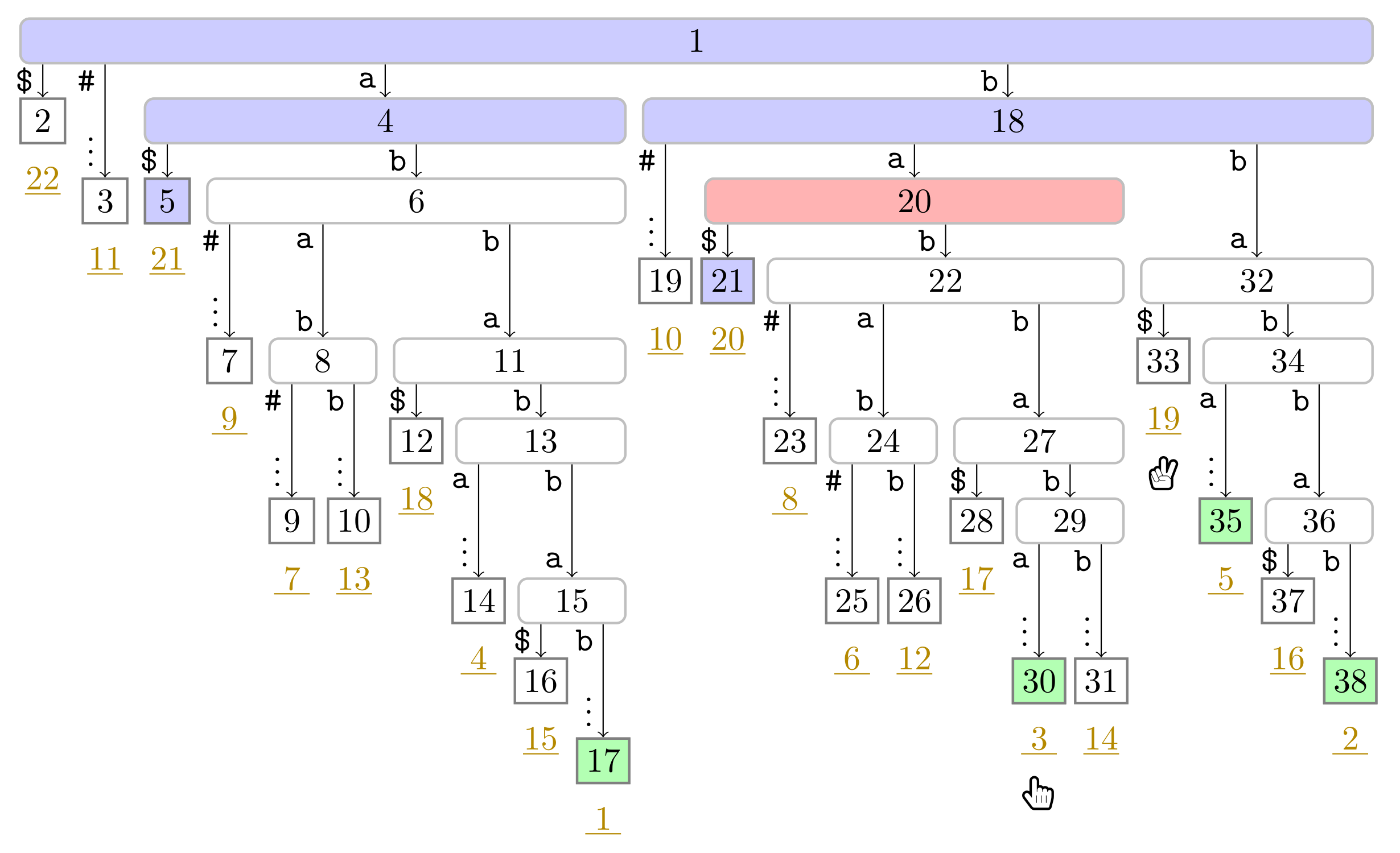
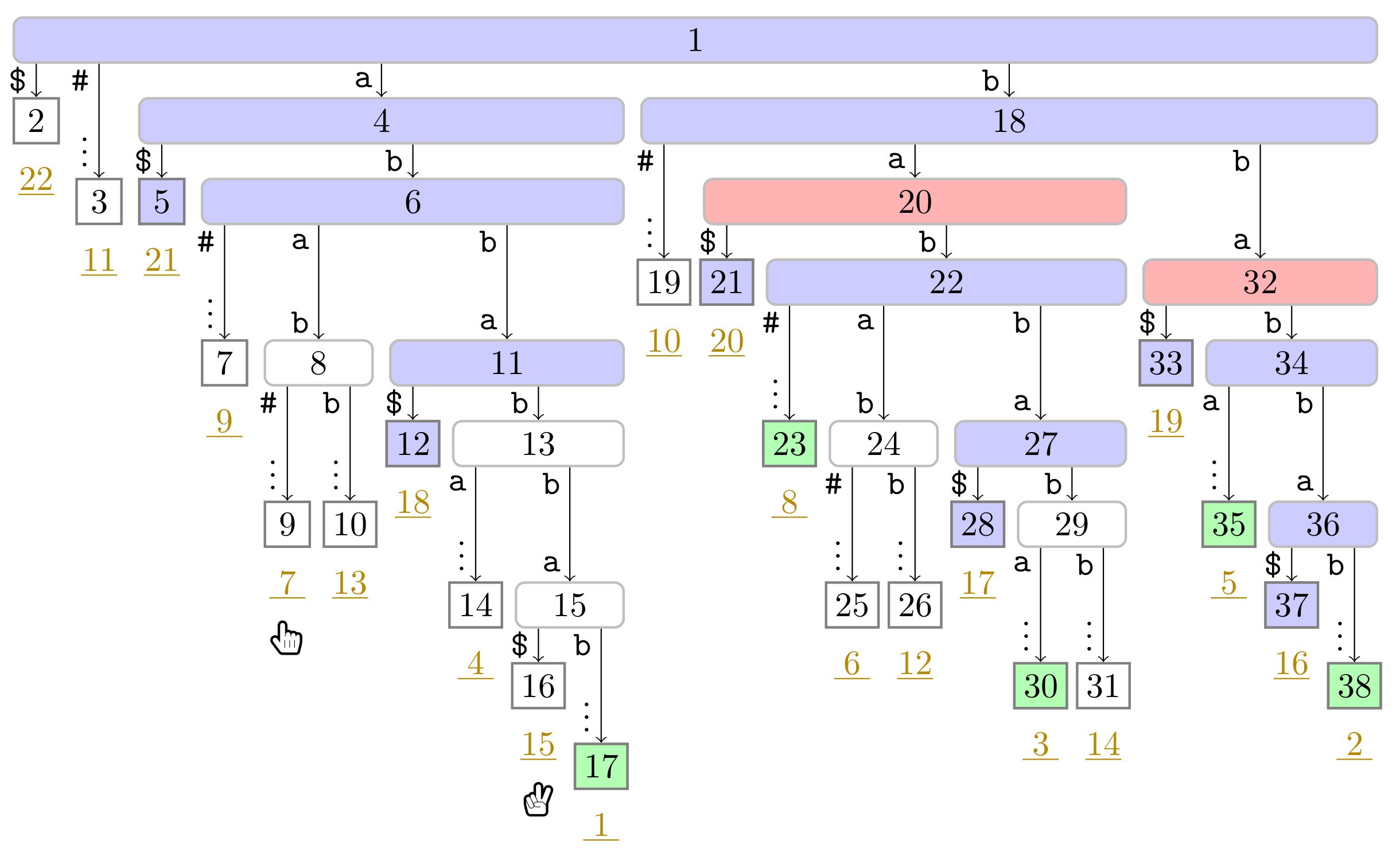
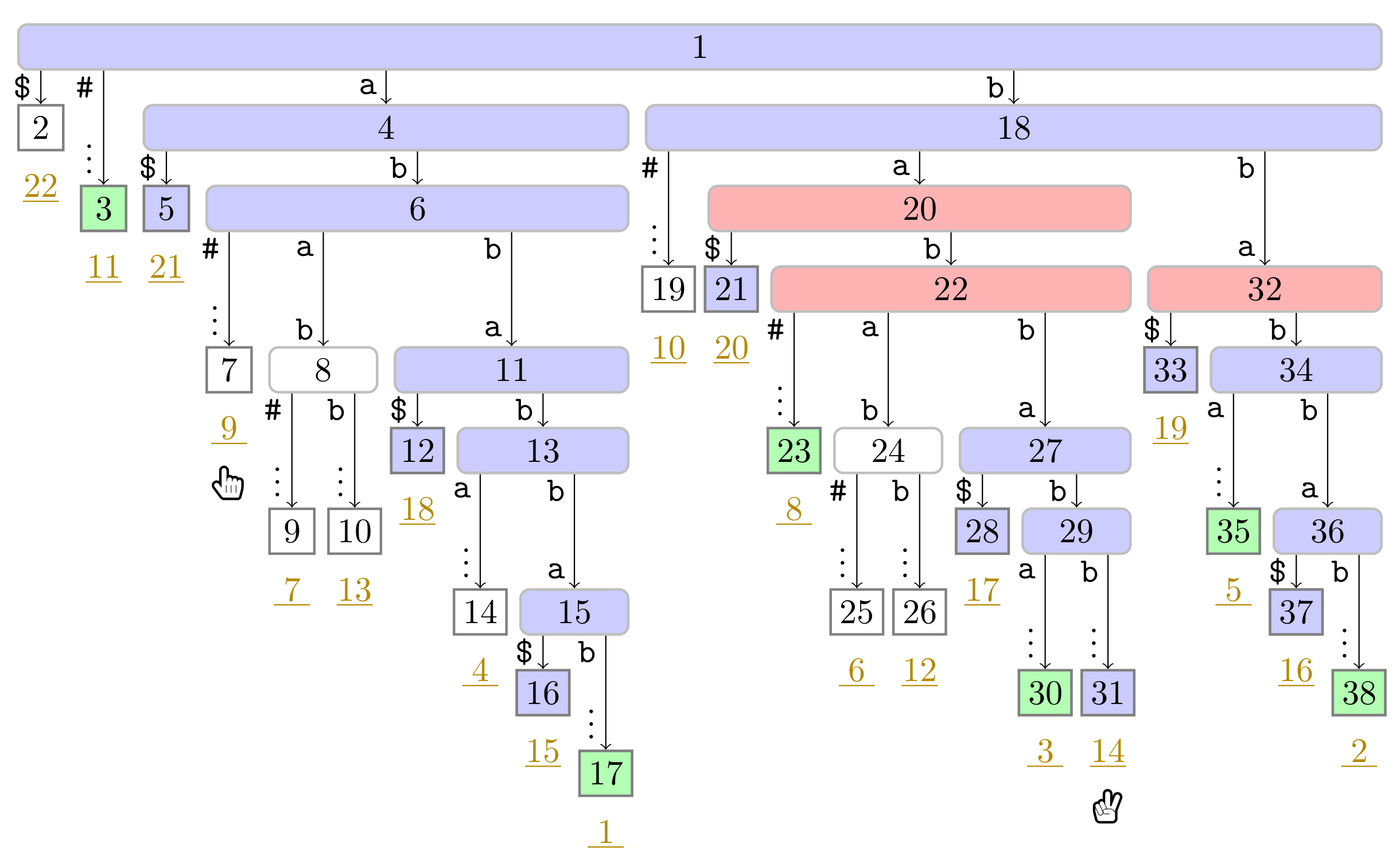
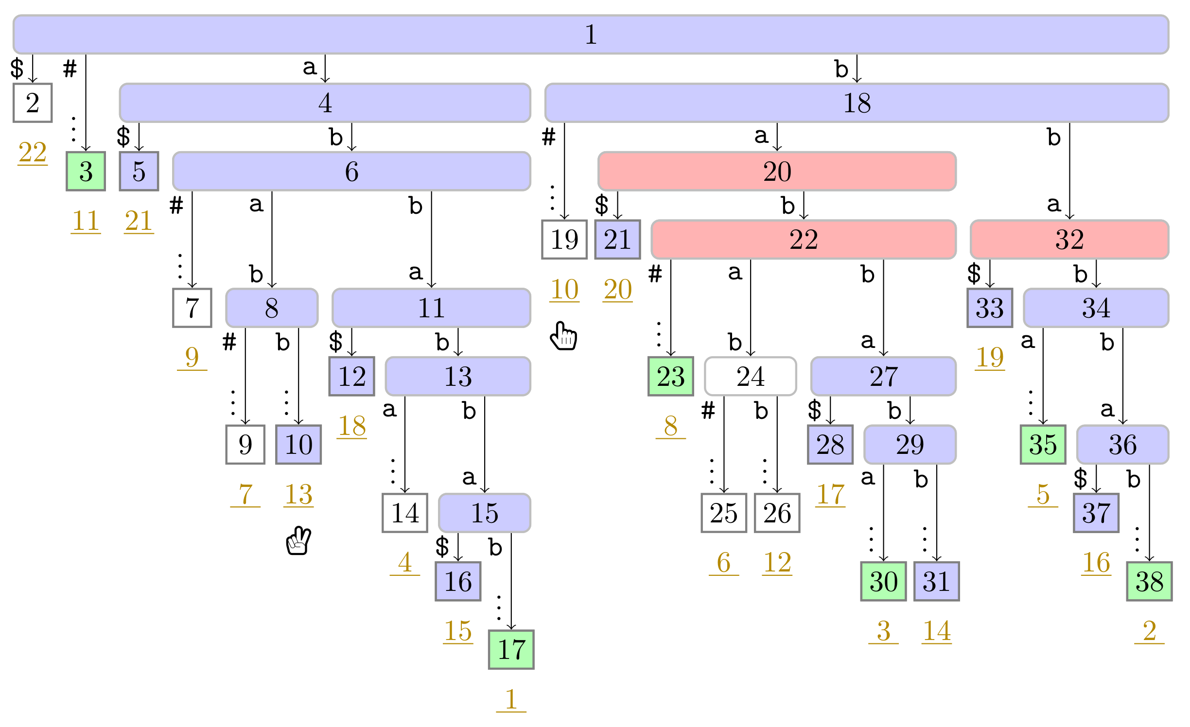
In this appendix, we provide a detailed execution of the algorithm sketched in Figure 4, Figure 5 and Figure 6 by showing the state per turn and per player in Figure A1, Figure A2, Figure A3, Figure A4, Figure A5, Figure A6, Figure A7, Figure A8, Figure A9, Figure A10, Figure A11, Figure A12, Figure A13, Figure A14, Figure A15, Figure A16, Figure A17, Figure A18, Figure A19, Figure A20 and Figure A21. In our running example, each player has 10 turns.
Figure A1. Flip Book: Initial State.
Algorithms 14 00161 g0a1
Figure A2. Flip Book: End of Turn 1 of Player 1.
Algorithms 14 00161 g0a2
Figure A3. Flip Book: End of Turn 1 of Player 2.
Algorithms 14 00161 g0a3
Figure A4. Flip Book: End of Turn 2 of Player 1.
Algorithms 14 00161 g0a4
Figure A5. Flip Book: End of Turn 2 of Player 2.
Algorithms 14 00161 g0a5
Figure A6. Flip Book: End of Turn 3 of Player 1.
Algorithms 14 00161 g0a6
Figure A7. Flip Book: End of Turn 3 of Player 2.
Algorithms 14 00161 g0a7
Figure A8. Flip Book: End of Turn 4 of Player 1.
Algorithms 14 00161 g0a8
Figure A9. Flip Book: End of Turn 4 of Player 2.
Algorithms 14 00161 g0a9
Figure A10. Flip Book: End of Turn 5 of Player 1.
Algorithms 14 00161 g0a10
Figure A11. Flip Book: End of Turn 5 of Player 2.
Algorithms 14 00161 g0a11
Figure A12. Flip Book: End of Turn 6 of Player 1.
Algorithms 14 00161 g0a12
Figure A13. Flip Book: End of Turn 6 of Player 2.
Algorithms 14 00161 g0a13
Figure A14. Flip Book: End of Turn 7 of Player 1.
Algorithms 14 00161 g0a14
Figure A15. Flip Book: End of Turn 7 of Player 2.
Algorithms 14 00161 g0a15
Figure A16. Flip Book: End of Turn 8 of Player 1.
Algorithms 14 00161 g0a16
Figure A17. Flip Book: End of Turn 8 of Player 2.
Algorithms 14 00161 g0a17
Figure A18. Flip Book: End of Turn 9 of Player 1.
Algorithms 14 00161 g0a18
Figure A19. Flip Book: End of Turn 9 of Player 2.
Algorithms 14 00161 g0a19
Figure A20. Flip Book: End of Turn 10 of Player 1.
Algorithms 14 00161 g0a20
Figure A21. Flip Book: End of Turn 10 of Player 2.
Algorithms 14 00161 g0a21

References

  1. Kolpakov, R.; Kucherov, G. Searching for gapped palindromes. Theor. Comput. Sci. 2009, 410, 5365–5373. [Google Scholar] [CrossRef] [Green Version]
  2. Storer, J.A.; Szymanski, T.G. Data compression via textural substitution. J. ACM 1982, 29, 928–951. [Google Scholar] [CrossRef]
  3. Crochemore, M.; Langiu, A.; Mignosi, F. Note on the greedy parsing optimality for dictionary-based text compression. Theor. Comput. Sci. 2014, 525, 55–59. [Google Scholar] [CrossRef]
  4. Weiner, P. Linear Pattern Matching Algorithms. In Proceedings of the 14th Annual Symposium on Switching and Automata Theory (swat 1973) SWAT, Iowa City, IA, USA, 15–17 October 1973; pp. 1–11. [Google Scholar]
  5. Sugimoto, S.; Tomohiro, I.; Inenaga, S.; Bannai, H.; Takeda, M. Computing Reversed Lempel–Ziv Factorization Online. Available online: http://stringology.org/papers/PSC2013.pdf#page=115 (accessed on 15 April 2021).
  6. Chairungsee, S.; Crochemore, M. Efficient Computing of Longest Previous Reverse Factors. In Proceedings of the Computer Science and Information Technologies, Yerevan, Armenia, 28 September–2 October 2009; pp. 27–30. [Google Scholar]
  7. Badkobeh, G.; Chairungsee, S.; Crochemore, M. Hunting Redundancies in Strings. In International Conference on Developments in Language Theory; LNCS; Springer: Berlin/Heidelberg, Germany, 2011; Volume 6795, pp. 1–14. [Google Scholar]
  8. Chairungsee, S. Searching for Gapped Palindrome. Available online: https://www.sciencedirect.com/science/article/pii/S0304397509006409 (accessed on 15 April 2021).
  9. Charoenrak, S.; Chairungsee, S. Palindrome Detection Using On-Line Position. In Proceedings of the 2017 International Conference on Information Technology, Singapore, 27–29 December 2017; pp. 62–65. [Google Scholar]
  10. Charoenrak, S.; Chairungsee, S. Algorithm for Palindrome Detection by Suffix Heap. In Proceedings of the 2019 7th International Conference on Information Technology: IoT and Smart City, Shanghai China, 20–23 December 2019; pp. 85–88. [Google Scholar]
  11. Blumer, A.; Blumer, J.; Ehrenfeucht, A.; Haussler, D.; McConnell, R.M. Building the Minimal DFA for the Set of all Subwords of a Word On-line in Linear Time. In International Colloquium on Automata, Languages, and Programming; LNCS; Springer: Berlin/Heidelberg, Germany, 1984; Volume 172, pp. 109–118. [Google Scholar]
  12. Ehrenfeucht, A.; McConnell, R.M.; Osheim, N.; Woo, S. Position heaps: A simple and dynamic text indexing data structure. J. Discret. Algorithms 2011, 9, 100–121. [Google Scholar] [CrossRef] [Green Version]
  13. Gagie, T.; Hon, W.; Ku, T. New Algorithms for Position Heaps. In Annual Symposium on Combinatorial Pattern Matching; LNCS; Springer: Berlin/Heidelberg, Germany, 2013; Volume 7922, pp. 95–106. [Google Scholar]
  14. Crochemore, M.; Iliopoulos, C.S.; Kubica, M.; Rytter, W.; Walen, T. Efficient algorithms for three variants of the LPF table. J. Discret. Algorithms 2012, 11, 51–61. [Google Scholar] [CrossRef] [Green Version]
  15. Manber, U.; Myers, E.W. Suffix Arrays: A New Method for On-Line String Searches. SIAM J. Comput. 1993, 22, 935–948. [Google Scholar] [CrossRef]
  16. Dumitran, M.; Gawrychowski, P.; Manea, F. Longest Gapped Repeats and Palindromes. Discret. Math. Theor. Comput. Sci. 2017, 19, 205–217. [Google Scholar]
  17. Gusfield, D. Algorithms on Strings, Trees, and Sequences: Computer Science and Computational Biology; Cambridge University Press: Cambridge, UK, 1997. [Google Scholar]
  18. Nakashima, Y.; Tomohiro, I.; Inenaga, S.; Bannai, H.; Takeda, M. Constructing LZ78 tries and position heaps in linear time for large alphabets. Inf. Process. Lett. 2015, 115, 655–659. [Google Scholar] [CrossRef] [Green Version]
  19. Ziv, J.; Lempel, A. A universal algorithm for sequential data compression. IEEE Trans. Inf. Theory 1977, 23, 337–343. [Google Scholar] [CrossRef] [Green Version]
  20. Ziv, J.; Lempel, A. Compression of individual sequences via variable-rate coding. IEEE Trans. Inf. Theory 1978, 24, 530–536. [Google Scholar] [CrossRef] [Green Version]
  21. Fischer, J.; Tomohiro, I; Köppl, D.; Sadakane, K. Lempel–Ziv Factorization Powered by Space Efficient Suffix Trees. Algorithmica 2018, 80, 2048–2081. [Google Scholar] [CrossRef]
  22. Köppl, D. Non-Overlapping LZ77 Factorization and LZ78 Substring Compression Queries with Suffix Trees. Algorithms 2021, 14, 44. [Google Scholar] [CrossRef]
  23. Sadakane, K. Compressed Suffix Trees with Full Functionality. Theory Comput. Syst. 2007, 41, 589–607. [Google Scholar] [CrossRef] [Green Version]
  24. Belazzougui, D.; Cunial, F. Indexed Matching Statistics and Shortest Unique Substrings. In International Symposium on String Processing and Information Retrieval; LNCS; Springer: Cham, Switzerland, 2014; Volume 8799, pp. 179–190. [Google Scholar]
  25. Franek, F.; Holub, J.; Smyth, W.F.; Xiao, X. Computing Quasi Suffix Arrays. J. Autom. Lang. Comb. 2003, 8, 593–606. [Google Scholar]
  26. Crochemore, M.; Ilie, L. Computing Longest Previous Factor in linear time and applications. Inf. Process. Lett. 2008, 106, 75–80. [Google Scholar] [CrossRef] [Green Version]
  27. Belazzougui, D.; Cunial, F.; Kärkkäinen, J.; Mäkinen, V. Linear-time String Indexing and Analysis in Small Space. ACM Trans. Algorithms 2020, 16, 17:1–17:54. [Google Scholar] [CrossRef]
  28. Goto, K.; Bannai, H. Space Efficient Linear Time Lempel–Ziv Factorization for Small Alphabets. In Proceedings of the 2014 Data Compression Conference, Snowbird, UT, USA, 26–28 March 2014; pp. 163–172. [Google Scholar]
  29. Kärkkäinen, J.; Kempa, D.; Puglisi, S.J. Lightweight Lempel–Ziv Parsing. In International Symposium on Experimental Algorithms; LNCS; Springer: Berlin/Heidelberg, Germany, 2013; Volume 7933, pp. 139–150. [Google Scholar]
  30. Kosolobov, D. Faster Lightweight Lempel–Ziv Parsing. In International Symposium on Mathematical Foundations of Computer Science; LNCS; Springer: Berlin/Heidelberg, Germany, 2015; Volume 9235, pp. 432–444. [Google Scholar]
  31. Belazzougui, D.; Puglisi, S.J. Range Predecessor and Lempel–Ziv Parsing. In Proceedings of the Twenty-Seventh Annual ACM-SIAM Symposium on Discrete Algorithms, Arlington, VA, USA, 10–12 January 2016; pp. 2053–2071. [Google Scholar]
  32. Okanohara, D.; Sadakane, K. An Online Algorithm for Finding the Longest Previous Factors. In European Symposium on Algorithms; LNCS; Springer: Berlin/Heidelberg, Germany, 2008; Volume 5193, pp. 696–707. [Google Scholar]
  33. Prezza, N.; Rosone, G. Faster Online Computation of the Succinct Longest Previous Factor Array. In Conference on Computability in Europe; LNCS; Springer: Cham, Switzerland, 2020; Volume 12098, pp. 339–352. [Google Scholar]
  34. Bannai, H.; Inenaga, S.; Köppl, D. Computing All Distinct Squares in Linear Time for Integer Alphabets. In Proceedings of the 28th Annual Symposium on Combinatorial Pattern Matching (CPM 2017), Warsaw, Poland, 4–6July 2017; Volume 78, LIPIcs. pp. 22:1–22:18. Available online: https://link.springer.com/chapter/10.1007/978-3-662-48057-1_16 (accessed on 16 April 2021).
  35. Jacobson, G. Space-efficient Static Trees and Graphs. In Proceedings of the 30th Annual Symposium on Foundations of Computer Science Research, Triangle Park, NC, USA, 30 October–1 November 1989; pp. 549–554. [Google Scholar]
  36. Clark, D.R. Compact Pat Trees. Ph.D. Thesis, University of Waterloo, Waterloo, ON, Canada, 1996. [Google Scholar]
  37. Baumann, T.; Hagerup, T. Rank-Select Indices Without Tears. In Proceedings of the Algorithms and Data Structures—16th International Symposium, WADS 2019, Edmonton, AB, Canada, 5–7 August 2019; LNCS. Volume 11646, pp. 85–98. [Google Scholar]
  38. Munro, J.I.; Navarro, G.; Nekrich, Y. Space-Efficient Construction of Compressed Indexes in Deterministic Linear Time. In Proceedings of the Twenty-Eighth Annual ACM-SIAM Symposium on Discrete Algorithms, Barcelona, Spain, 16–19 January 2017; pp. 408–424. [Google Scholar]
  39. Burrows, M.; Wheeler, D.J. A Block Sorting Lossless Data Compression Algorithm; Technical Report 124; Digital Equipment Corporation: Palo Alto, CA, USA, 1994. [Google Scholar]
  40. Lempel, A.; Ziv, J. On the Complexity of Finite Sequences. IEEE Trans. Inf. Theory 1976, 22, 75–81. [Google Scholar] [CrossRef]
  41. Fischer, J.; Mäkinen, V.; Navarro, G. Faster entropy-bounded compressed suffix trees. Theor. Comput. Sci. 2009, 410, 5354–5364. [Google Scholar] [CrossRef] [Green Version]
  42. Manacher, G.K. A New Linear-Time “On-Line” Algorithm for Finding the Smallest Initial Palindrome of a String. J. ACM 1975, 22, 346–351. [Google Scholar] [CrossRef]
  43. Apostolico, A.; Breslauer, D.; Galil, Z. Parallel Detection of all Palindromes in a String. Theor. Comput. Sci. 1995, 141, 163–173. [Google Scholar] [CrossRef] [Green Version]
  44. Köppl, D. Exploring Regular Structures in Strings. Ph.D. Thesis, TU Dortmund, Dortmund, Germany, 2018. [Google Scholar]
  45. Grossi, R.; Vitter, J.S. Compressed Suffix Arrays and Suffix Trees with Applications to Text Indexing and String Matching. SIAM J. Comput. 2005, 35, 378–407. [Google Scholar] [CrossRef]
  46. Fleischer, L.; Shallit, J.O. Words Avoiding Reversed Factors, Revisited. arXiv 2019, arXiv:1911.11704. [Google Scholar]
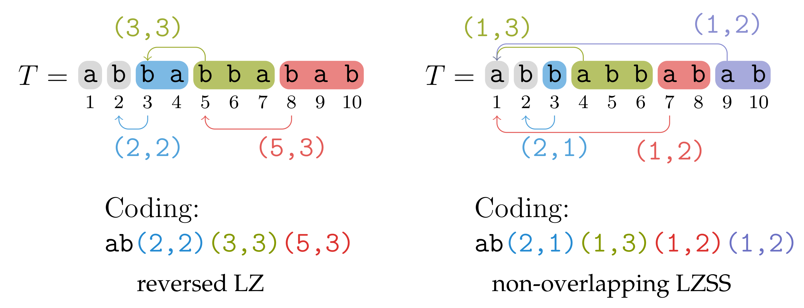
Figure 1. The reversed LZ and the non-overlapping LZSS factorization of the string T = abbabbabab . A factor F is visualized by a rounded rectangle. Its coding consists of a mere character if it has no reference; otherwise, its coding consists of its referred position p and its length such that F = T [ p + 1 . . p ] R for the reversed LZ factorization, and F = T [ p . . p + 1 ] for the non-overlapping LZSS factorization.
Algorithms 14 00161 g001
Figure 2. Witness node w of a referencing factor F starting at text position i. Given j is the referred position of F, the witness w of F is the node in the suffix tree having (a) F as a prefix of its string label and (b) the leaves with suffix numbers 2 n j and i in its subtree. lemWitness shows that w is uniquely defined to be the node whose string label is F.
Algorithms 14 00161 g002
Figure 3. A reversed-LZ factor F starting at position i in R with a referred position j | F | + 1 . If a = a ¯ with a , a ¯ Σ , then we could extend F by one character, contradicting its definition to be the longest prefix of T [ i . . ] whose reverse occurs in T [ 1 . . i 1 ] . Hence, a a ¯ and F is a right-maximal repeat.
Algorithms 14 00161 g003
Figure 4. Suffix tree of T # · T R · $ used in Section 3.2, where T = abbabbabab is our running example. The nodes are labeled by their preorder numbers. The suffix number of each leaf λ is the underlined number drawn in dark yellow below λ . We trimmed the label of each edge to a leaf having more than two characters and display only the first character and the vertical dots ‘⋮’ as a sign of omission. The tree shows the state of Algorithm 1 after the first turn of both players. The nodes visited by Player 2 are colored in blue ( Algorithms 14 00161 i003), the phrase leaves are colored in green ( Algorithms 14 00161 i004). Player 1 and 2 are represented by the hands Algorithms 14 00161 i005 and Algorithms 14 00161 i006, respectively, pointing to the respective leaves they visited during the first turn.
Algorithms 14 00161 g004
Figure 5. Continuation of Figure 4 with the state at the fifth turn of Player 1. Additionally to the coloring used in Figure 4, witnesses are colored in red ( Algorithms 14 00161 i007). In this figure, Player 1 just finished her turn on making the node with preorder number 32 the witness w of the leaf with suffix number 5. With w we know that the factor starting at text position 5 has the length str _ depth ( w ) and that the next phrase leaf has suffix number 8. For visualization purposes, we left the hand ( Algorithms 14 00161 i006) of Player 2 below the leaf of her last turn.
Algorithms 14 00161 g005
Figure 6. State of our running example at termination of Algorithm 1. We have computed the bit vector B L of length n = 11 storing a one at the entries 1 , 2 , 3 , 5 , and 8, i.e., the suffix numbers of the phrase leaves, which are marked in green ( Algorithms 14 00161 i004), and the bit vector B W of length 38 (the maximum preorder number of an ST node) storing a one at the entries 20 , 22 , and 32, i.e., the preorder numbers of the witnesses, which are colored red ( Algorithms 14 00161 i007). During the second pass described in Section 3.3, we compute W storing the referred positions in the order of the witness ranks (left table).
Algorithms 14 00161 g006
Figure 7. Setting of Section 4.1. Nodes marked in B V are colored in blue ( Algorithms 14 00161 i003). Curly arcs symbolize paths that can visit multiple nodes (which are not visualized). When visiting the lowest ancestor of λ marked in B V for computing LPnrF [ i 1 ] , Player 1 determines w ˜ = suffixlink ( w ) such that she can skip the nodes on the path from the root to the leaf λ ˜ for computing LPnrF [ i ] (these nodes are symbolized by the curly arc highlighted in yellow ( Algorithms 14 00161 i008) on the right). There are leaves λ R and λ ˜ R with suffix numbers of at least 2 n i + 2 and 2 n i + 3 , respectively, since otherwise w would not have been marked in B V by Player 2.
Algorithms 14 00161 g007
Figure 8. Computing LPnrF with [14] ([Algorithm 2]) as explained in Section 4.2. Starting at the leaf λ R , we jump to the leftmost leaf λ with lca ( λ , λ ) = lca ( λ R , λ ) . Then, we use the operation max _ sufnum ( I ) returning the leaf-rank of the leaf λ R having the largest suffix number among the query interval I = [ leaf _ rank ( λ ) + 1 . . leaf _ rank ( λ ) 1 ] . If sufnum ( λ R ) > 2 n i , we recurse by setting λ R λ R . The LCA of λ R and λ is at least as deep as the child v of u on the path towards λ (the figure shows the case that v = lca ( λ R , λ ) ), and hence R [ i ] is at least str _ depth ( v ) if we recurse.
Algorithms 14 00161 g008
Table 1. Complexity bounds of related approaches described in Section 1.2 for a selectable parameter ϵ ( 0 , 1 ] .
( 1 + ϵ ) n lg n + O ( n ) Bits of Working Space (Excluding the Read-Only Text T)
ReferenceTypeTime
[21] ([Corollary 3.7])overlapping LZSS O ( ϵ 1 n )
[34] ([Lemma 6]) LPF O ( ϵ 1 n )
[22] ([Theorem 1])non-overlapping LZSS O ( ϵ 1 n )
[22] ([Theorem 3]) LPnF O ( ϵ 1 n )
O ( ϵ 1 n lg σ ) Bits of Working Space
ReferenceTypeTime
[21] ([Corollary 3.4])overlapping LZSS O ( ϵ 1 n )
[34] ([Lemma 6]) LPF O ( ϵ 1 n log σ ϵ n )
[22] ([Theorem 1])non-overlapping LZSS O ( ϵ 1 n log σ ϵ n )
[22] ([Theorem 3]) LPnF O ( ϵ 1 n log σ ϵ n )
Table 2. Construction time and needed space in bits for the succinct suffix tree (SST) and compressed suffix tree (CST) representations, cf. [21] ([Section 2.2]).
SSTCST
Time O ( n / ϵ ) O ( ϵ 1 n )
Space ( 2 + ϵ ) n lg n + O ( n ) O ( ϵ 1 n lg σ )
Table 3. Time bounds for certain operations needed by our LZ factorization algorithms. Although not explicitly mentioned in [21], the time for prev _ leaf is obtained with the Burrows–Wheeler transform [39] stored in the CST [38] ([A.1]) by constant-time partial rank queries, see [27] ([Section 3.4]) or [38] ([A.4]).
OperationSST TimeCST Time
sufnum ( λ ) O ( 1 / ϵ ) O ( n )
str _ depth ( v ) O ( 1 / ϵ ) O ( str _ depth ( v ) )
suffixlink ( v ) O ( 1 / ϵ ) O ( 1 )
prev _ leaf O ( 1 / ϵ ) O ( 1 )
Table 4. LPnrF and LPnF of our running example. Both arrays are defined in Section 4. See Section 5 for the definition of LPrF .
i1234567891011
T # abbabbabab#
LPnrF 00213323210
LPnF 00133323210
LPrF 06554323210
Publisher’s Note: MDPI stays neutral with regard to jurisdictional claims in published maps and institutional affiliations.