Identification of Intrinsically Disordered Protein Regions Based on Deep Neural Network-VGG16

Abstract

The accurate of i identificationntrinsically disordered proteins or protein regions is of great importance, as they are involved in critical biological process and related to various human diseases. In this paper, we develop a deep neural network that is based on the well-known VGG16. Our deep neural network is then trained through using 1450 proteins from the dataset DIS1616 and the trained neural network is tested on the remaining 166 proteins. Our trained neural network is also tested on the blind test set R80 and MXD494 to further demonstrate the performance of our model. The $MCC$ value of our trained deep neural network is $0.5132$ on the test set DIS166, $0.5270$ on the blind test set R80 and $0.4577$ on the blind test set MXD494. All of these $MCC$ values of our trained deep neural network exceed the corresponding values of existing prediction methods.

1. Introduction

The intrinsically disordered proteins (IDPs) have at least one region that do not have stable three-dimensional structure [1,2,3], and they are widespread in nature [4]. IDPs are involved in key biological processes, such as the folding of nucleic acids, transcription and translation, protein–protein interactions, protein–RNA interactions, etc. [5,6,7]. Besides, IDPs are related to many human diseases, such as cancer, Alzheimer’s disease, cardiovascular disease, and various genetic diseases [8,9]. Therefore, the accurate identification of IDPs is crucial for the study of protein structure, function, and drug design. In the past few decades, various experimental methods have been proposed to identify IDPs, such as nuclear magnetic resonance (NMR), X-ray crystallography, and circular dichroism (CD) [10,11]. However, it is expensive and time-consuming to identify disordered proteins through experiments, so numerous computational methods have been proposed to predict disordered proteins.

The available computational methods can be broadly classified into three categories: (1) scoring function-based methods. Methods in this category use a function to predict the propensity for disorder. Furthermore, they commonly employ the physiochemical properties of individual amino acids in the protein chain as its input. Example methods include IsUnstruct [12], GlobPlot [13], FoldUnfold [14], and IUPred [15], etc. (2) Machine learning-based methods. In this category, predictive models that are generated by machine learning algorithms (such as neural networks and support vector machines) are used to calculate the disorder tendencies. Typically, these predictive models use physiochemical properties of amino acid, evolutionary information, and solvent accessibility as inputs. These include RFPR-IDP [16], IDP-Seq2Seq [17], SPOT-Disorder [18], SPOT-Disorder2 [19], DISOPRED3 [20], SPINE-D [21], and ESpritz [22]. (3) Meta methods. They include MFDp [23], MetaDisorder [24], and MetaPrDOS [25]. These methods combine the results of multiple predictors to obtain the optimal prediction of IDPs.

Because traditional machine learning-based methods do not efficiently capture local patterns between amino-acids, we chose to use CNN as our network structure, which is known to be relatively lighter than other neural networks (e.g., recurrent neural networks), and it is effective in capturing local patterns [26,27]. In this paper, to capture the patterns of features in more detail, we develop a deep neural network that is comprised of ten identical deep neural structures, with each of them being derived from the original VGG16 model [28] and a MLP network, as shown in Figure 1. Each of these ten identical deep neural architectures is identical to the VGG16 model with no the fully-connected (FC) layer. The outputs of these structures are then used as the inputs of our MLP network for classification, where our MLP consists of two hidden layers with 512 perceptrons in each layer and uses cross entropy as its loss function. Subsequently, we randomly subdivide the dataset DIS1616 [29] into two disjoint subsets with one containing 1450 proteins for training and the other DIS166 having the remaining 166 proteins for testing. The ten-fold cross validation is performed on the training dataset DIS1450. On the test set DIS166 and blind test sets R80 [30] and MXD494 [31], the performance of our trained deep neural network is compared to two recent prediction methods that claim to have the best performances, i.e., RFPR-IDP and SPOT-Disorder 2. The $MCC$ value of our trained deep neural network is $0.5132$ on the test set DIS166, $0.5270$ on the blind test set R80 and $0.4577$ on the blind test set MXD494. All of these $MCC$ values from our trained deep neural network exceed the corresponding values of RFPR-IDP and SPOT-Disorder2.

2. Materials and Methods

In this section, we utilize the neural structure VGG16 and develop a deep neural network for identifying IDPs. Our deep neural structure comprises ten variant VGG16 and a MLP network.

2.1. Datasets

The first dataset we use through out this paper is DIS1616 of the DisProt database [29], which contains 182,316 disordered amino-acids and 706,362 ordered amino-acids. Here, we randomly split the set DIS1616 of 1616 proteins into two disjoint subsets with one (referred to DIS1450) containing 1450 proteins for training and the other (referred to DIS166) having the remaining 166 proteins for testing. Subsequently the ten-fold cross validation is performed on the training dataset DIS1450. To further demonstrate the performance of our trained deep neural network, we use the datasets R80 and MXD494 as blind test sets, where R80 consists of 3566 disordered amino-acids and 29,243 ordered amino-acids, and MXD494 consists of 44,087 disordered amino-acids and 152,414 ordered amino-acids.

2.2. Pre-Processing the Features of Proteins for the Input of Our Model

The input features of our deep neural network can be classified into three types, i.e., the physicochemical properties, evolutionary information, and amino acid propensities. The physicochemical parameters [32] we use are steric parameter, polarizability, volume, hydrophobicity, isoelectric point, helix, and sheet probability. The evolutionary information is a 20-dimensional position-specific substitution matrix (PSSM) [33] derived from the Position-Specific Iterative Basic Local Alignment Search Tool (PSI-BLAST) [34]. Three propensities of amino-acids are from GlobPlot NAR paper.

The procedure of pre-processing proceeds, as follows:

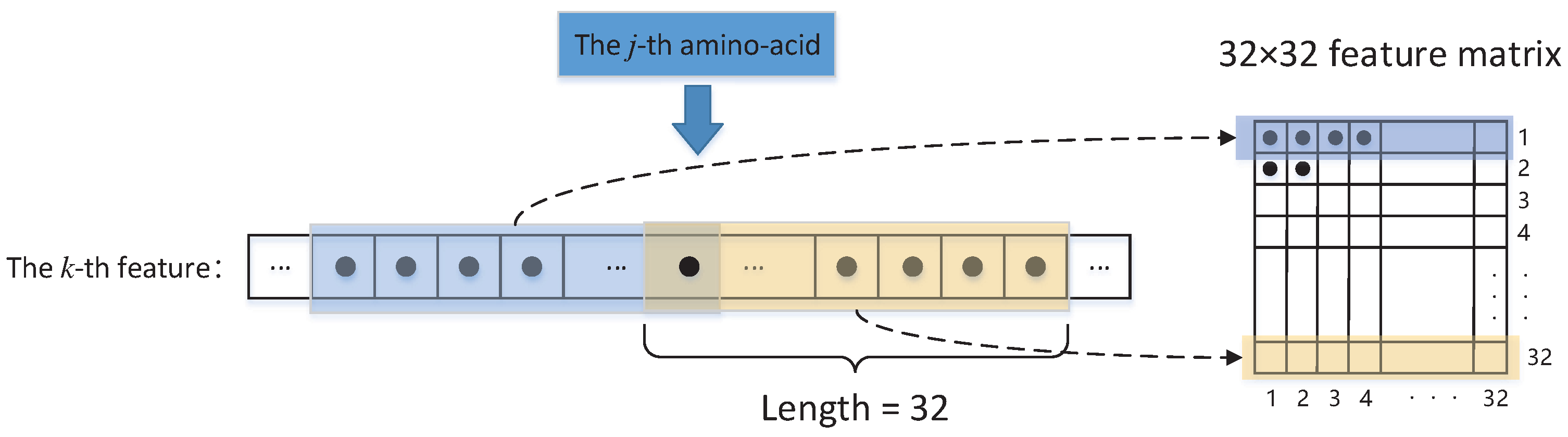
• Given an amino-acid sequence of a protein of size L, we use a sliding window of size 21 and, for each amino-acid in the sliding window, compute the physicochemical properties, evolutionary information, and amino-acid propensities that are defined in the above paragraph. These computed feature values of amino-acids are then averaged over our sliding window and used to represent the feature value of the amino-acid in the center of our sliding window. For two terminal amino-acids of a protein, we append 10 zeros on the left and right side of the amino-acid sequence of a protein, respectively. Thus, for each amino-acid sequence of a protein, we can associate it with a $30\times L$ feature matrix

  $$\mathbf{F}=[{\mathbf{x}}_1{\mathbf{x}}_2\cdots {\mathbf{x}}_L],$$

  (1)

  where the entries of vector ${\mathbf{x}}_j(1\le j\le L)$ represents the feature values (seven physicochemical properties, twenty entries of a column in the PSSM matrix, and 3 amino-acid propensities) associated with the j-th amino-acid. Assume that a $30\times 1$ vector ${\mathbf{x}}_j(1\le j\le L)$ can be denoted by

  $${\mathbf{x}}_j={[m_{1,j}{m}_{2,j}\cdots m_{30,j}]}^{\mathrm{T}},$$

  (2)

  where $m_{k,j}$ is the k-th feature value $(1\le k\le 30)$ that is associated with the j-th amino-acid $(1\le j\le L)$ averaged over the sliding window of size 21.
• Because the minimum input size of the VGG16 is required to be $32\times 32\times 3$, we transfer the $30\times L$ feature matrix to three matrices of size $32\times 32$, as Figure 2 depicts. That is, for each feature vector $m_{k,j}$$1\le k\le 30$ and $1\le j\le L$ defined in (2), we introduce an associated $32\times 32$ matrix ${\mathbf{w}}_{k,j}$, which is

  $$\begin{array}{cc}\hfill {\mathbf{w}}_{k,j}& =\left[\begin{array}{c}\mathbf{F}(k,j-31:j)\\ \mathbf{F}(k,j-30:j+1)\\ ⋮\\ \mathbf{F}(k,j:j+31)\end{array}\right]=\left[\begin{array}{cccc}{m}_{k,(j-31)}& m_{k,(j-30)}& \cdots & m_{k,j}\\ m_{k,(j-30)}& m_{k,(j-29)}& \cdots & m_{k,(j+1)}\\ ⋮& ⋮& \ddots & ⋮\\ m_{k,j}& m_{k,(j+1)}& \cdots & m_{k,(j+31)}\end{array}\right],\hfill \end{array}$$

  (3)

  where $m_{k,j}=0$ with $j<1$ or $j>L$.
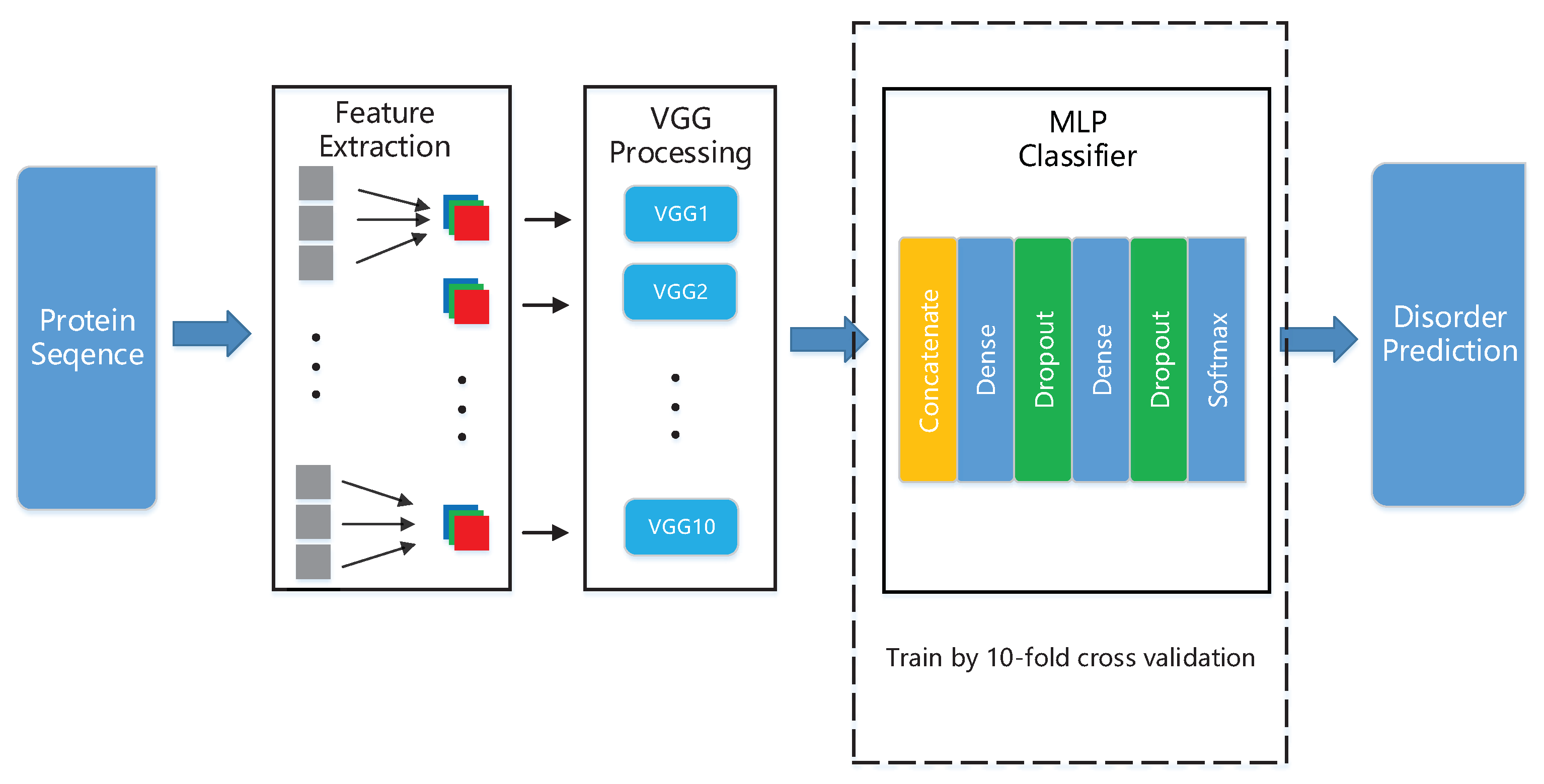
• Thus, for the j-th amino-acid, its thirty input features yield a sequence of $32\times 32$ matrices ${\mathbf{w}}_{1,j},{\mathbf{w}}_{2,j}\cdots {\mathbf{w}}_{30,j}$. Therefore, at each step, we choose three consecutive from the sequence of matrices ${\mathbf{w}}_{1,j},{\mathbf{w}}_{2,j}\cdots {\mathbf{w}}_{30,j}$ as the input of VGG16 network.

2.3. Designing and Training Our Deep Neural Network

The overall architecture of our deep neural network is comprised of ten identical deep neural structures, with each of them being derived from the original VGG16 model and a MLP network. Each of these ten identical deep neural architectures shown in Figure 3 only utilizes the convolutional blocks of the original VGG16 model, i.e., erasing the fully-connected (FC) layer of VGG16, but preserving the remaining VGG16 model as well as its associated weights and bias. The outputs of these ten identical deep neural structures are then used as the inputs of our constructed MLP network for classification.

The MLP network that we construct is a fully-connected MLP network with two layers, which employs the loss function defined as

$$Loss=\frac{1}{m}\sum _{i=1}^m[-({\alpha }_1{y}^{\left(i\right)}log\left({\widehat{y}}^{\left(i\right)}\right)+{\alpha }_2(1-y^{\left(i\right)})log(1-{\widehat{y}}^{\left(i\right)}))],$$

(4)

where m represents the batch size, i.e., the number of amino-acids used in each iteration during the training. $y^{\left(i\right)}$ is a binary indicator (0 or 1) with 1, which suggests that the i-th amino-acid is disordered and 0 indicating that it is ordered. ${\widehat{y}}^{\left(i\right)}$ is the predicted probability of the output $y^{\left(i\right)}=1$. Similarly, $1-{\widehat{y}}^{\left(i\right)}$ denotes the predicted probability of $y^{\left(i\right)}=0$. Parameter ${\alpha }_1$ and ${\alpha }_2$ are the weights computed through

$${\alpha }_1=\frac{N_{ord}}{N_{ord}+N_{dis}},$$

(5)

$${\alpha }_2=\frac{N_{dis}}{N_{ord}+N_{dis}},$$

(6)

where $N_{ord}$ and $N_{dis}$ correspond to the number of the ordered and disordered amino-acids in the training dataset, respectively.

Because we obtain a $1\times 1\times 512$ matrix from each our VGG16 output, ten $1\times 1\times 512$ matrices are obtained from our deep neural network. Each of these $1\times 1\times 512$ matrices are first flattened into a $1\times 512$ vector using the flattening layer. Subsequently, the concatenation function from Keras framework [35] is utilized to concatenate these ten $1\times 512$ vectors into a $1\times 5120$ vector as the input to our MLP network. Each of two hidden layers of our MLP network contains 512 perceptrons and the activation functions for these two hidden layers are chosen to be the rectified linear unit (ReLU). Moreover, we employ the dropout algorithm [36], with a dropout percentage of $50\%$ in each hidden layer of our MLP, to reduce overfitting. The output layer of our MLP network contains 2 perceptrons and it employs softmax as the activation function. The softmax activation function is defined as

$$f\left(s_p^{\left(i\right)}\right)=\frac{e^{s_p^{\left(i\right)}}}{e^{s_1^{\left(i\right)}}+e^{s_2^{\left(i\right)}}}(p=1,2),$$

(7)

where $s_p^{\left(i\right)}$ represents the p-th perceptron output value of the i-th amino-acid. The predicted probability of the output $y^{\left(i\right)}=1$ is defined as

$$f\left(s_1^{\left(i\right)}\right)=\frac{e^{s_1^{\left(i\right)}}}{e^{s_1^{\left(i\right)}}+e^{s_2^{\left(i\right)}}}={\widehat{y}}^{\left(i\right)}.$$

(8)

Similarly, the predicted probability of the output $y^{\left(i\right)}=0$ is defined as

$$f\left(s_2^{\left(i\right)}\right)=\frac{e^{s_2^{\left(i\right)}}}{e^{s_1^{\left(i\right)}}+e^{s_2^{\left(i\right)}}}=1-{\widehat{y}}^{\left(i\right)}.$$

(9)

We randomly subdivide the amino-acids of our training dataset DIS1450 into disjoint batches with each containing 128 amino-acids. The training process proceeds, as follows: for each amino-acid in a given batch, we use our deep neural network to compute the predicted probabilities that are defined in (8) and (9). Once we compute all of the predicted probabilities in this given batch, we then utilize Equation (4) to estimate the average loss of this batch. This computed average loss of the batch is employed to update the weights and bias of our MLP network through the Adam algorithm [37], where the initial learning rate of $0.0005$ is chosen to perform the back propagation and updating. The above process is repeated for each batch until all of the batches have been exhausted, which is referred as an epoch. Subsequently, we randomly subdivide the amino-acids of our training dataset DIS1450 again into disjoint batches with each containing 128 amino-acids and then repeat the above procedure until the loss function stops convergence or the maximum number of epochs is reached. Figure 4 shows the learning curve of the model.

The predicted probabilities defined in (8) and (9) we obtain after completing the training are used for determining whether i-th amino-acid is ordered or disordered where the majority-voting principle is employed.

2.4. Performance Evaluation

The performance of the IDPs prediction is evaluated through sensitivity ($Sens$), specificity ($Spec$), binary accuracy ($BACC$), and Matthews correlation coefficient ($MCC$). The formulae for computing $Sens$, $Spec$, $BACC$, and $MCC$ are

$$Sens=\frac{TP}{TP+FN},$$

(10)

$$Spec=\frac{TN}{TN+FP},$$

(11)

$$BACC=\frac{1}{2}(\frac{TP}{TP+FN}+\frac{TN}{TN+FP}),$$

(12)

$$MCC=\frac{(TP\times TN)-(FP\times FN)}{\sqrt{(TP+FP)(TP+FN)(TN+FP)(TN+FN)}}.$$

(13)

In these equations, $TP$, $FP$, $TN$, and $FN$, respectively, represent true positives (correctly predicted disordered residues), false positives (ordered residues that are incorrectly identified as disordered residues), true negatives (correctly predicted ordered residues), and false negatives (disordered residues that are incorrectly identified as ordered residues), respectively. The values of $MCC$ fall in $-1$ and $+1$, where 0 indicates a lack of correlation. The higher the $MCC$ values, the better the prediction.

3. Results and Discussion

Throughout the rest of this paper, DISvgg is used as the abbreviation of our deep neural network. Our DISvgg is compared with two recent prediction methods that claim to have the best performances, i.e., RFPR-IDP (available at http://bliulab.net/RFPR-IDP/server (accessed on 26 March 2021)) and SPOT-Disorder2 (available at https://sparks-lab.org/server/spot-disorder2/ (accessed on 26 March 2021)). The ten-fold cross validation is performed on the training dataset DIS1450. On the test set DIS166 and blind test set R80 and MXD494, the performance of our trained deep neural network is compared to two recent prediction methods that claim to have the best performances, i.e., RFPR-IDP and SPOT-Disorder2. The $MCC$ value of our trained deep neural network is $0.5132$ on the test set DIS166, $0.5270$ on the blind test set R80 and $0.4577$ on the blind test set MXD494. All of these $MCC$ values from our trained deep neural network exceed the corresponding values of RFPR-IDP and SPOT-Disorder2.

Table 1. Performance Parameters on Test Dataset DIS166.

Methods	Sens	Spec	BACC	MCC
DISvgg	0.6713	0.8828	0.7771	0.5132
RFPR-IDP	0.7557	0.7817	0.7687	0.4406
SPOT-Disorder2	0.7103	0.8084	0.7594	0.4952

,

Table 2. Performance Parameters on Blind Test Dataset R80.

Methods	Sens	Spec	BACC	MCC
DISvgg	0.5993	0.9429	0.7711	0.5270
RFPR-IDP	0.5464	0.9546	0.7505	0.5139
SPOT-Disorder2	0.4941	0.9439	0.7190	0.4486

and

Table 3. Performance Parameters on Blind Test Dataset MXD494.

Methods	Sens	Spec	BACC	MCC
DISvgg	0.7160	0.7956	0.7558	0.4577
RFPR-IDP	0.7490	0.7580	0.7540	0.4420
SPOT-Disorder2	0.6380	0.8200	0.7290	0.4482

list all of the related values for evaluating the performance on the test set DIS166 and blind test set R80 and MXD494.

The Performance Comparison on the Test Dataset DIS166 and Blind Test Datasets

In this section, we present the simulation results that were obtained from applying our trained DISvgg as well as some existing prediction methods, such as RFPR-IDP and SPOT-Disorder2, on the independent dataset DIS166 as well as blind test datasets R80 and MXD494. Table 1, Table 2 and Table 3 summarize all of the values used for evaluating the performance of prediction methods.

4. Conclusions

The accurate identification of intrinsically disordered proteins or protein regions is of great importance, as they are involved in critical biological processes and related to various human diseases. In this paper, we develop a deep neural network that is based on the well-known VGG16. Our deep neural network is then trained through using 1450 proteins from the dataset DIS1616 and the trained neural network is tested on the remaining 166 proteins. Our trained neural network is also tested on the blind test sets R80 and MXD494 to further demonstrate the performance of our model. The $MCC$ value of our trained deep neural network is $0.5132$ on the test set DIS166, $0.5270$ on the blind test set R80, and $0.4577$ on the blind test set MXD494. All of these $MCC$ values of our trained deep neural network exceed the corresponding values of existing prediction methods.

References

1. Uversky, V.N. The mysterious unfoldome: Structureless, underappreciated, yet vital part of any given proteome. J. Biomed. Biotechnol. 2010, 2010, 568068. [Google Scholar] [CrossRef] [PubMed]
2. Lieutaud, P.; Ferron, F.; Uversky, A.V.; Kurgan, L.; Uversky, V.N.; Longhi, S. How disordered is my protein and what is its disorder for? A guide through the “dark side” of the protein universe. Intrinsically Disord. Proteins 2016, 4, e1259708. [Google Scholar] [CrossRef] [Green Version]
3. Liu, Y.; Wang, X.; Liu, B. A comprehensive review and comparison of existing computational methods for intrinsically disordered protein and region prediction. Brief. Bioinform. 2019, 20, 330–346. [Google Scholar] [CrossRef] [PubMed]
4. Meng, F.; Uversky, V.; Kurgan, L. Computational prediction of intrinsic disorder in proteins. Curr. Protoc. Protein Sci. 2017, 88, 2–16. [Google Scholar] [CrossRef]
5. Uversky, V.N. Functional roles of transiently and intrinsically disordered regions within proteins. FEBS J. 2015, 282, 1182–1189. [Google Scholar] [CrossRef]
6. Holmstrom, E.D.; Liu, Z.; Nettels, D.; Best, R.B.; Schuler, B. Disordered RNA chaperones can enhance nucleic acid folding via local charge screening. Nat. Commun. 2019, 10, 1–11. [Google Scholar] [CrossRef] [PubMed]
7. Wright, P.E.; Dyson, H.J. Intrinsically disordered proteins in cellular signalling and regulation. Nat. Rev. Mol. Cell Biol. 2015, 16, 18–29. [Google Scholar] [CrossRef] [PubMed]
8. Kulkarni, V.; Kulkarni, P. Intrinsically disordered proteins and phenotypic switching: Implications in cancer. Prog. Mol. Biol. Transl. Sci. 2019, 166, 63–84. [Google Scholar] [PubMed]
9. Buljan, M.; Chalancon, G.; Dunker, A.K.; Bateman, A.; Balaji, S.; Fuxreiter, M.; Babu, M.M. Alternative splicing of intrinsically disordered regions and rewiring of protein interactions. Curr. Opin. Struct. Biol. 2013, 23, 443–450. [Google Scholar] [CrossRef] [PubMed]
10. Konrat, R. NMR contributions to structural dynamics studies of intrinsically disordered proteins. J. Magn. Reson. 2014, 241, 74–85. [Google Scholar] [CrossRef] [Green Version]
11. Oldfield, C.J.; Ulrich, E.L.; Cheng, Y.; Dunker, A.K.; Markley, J.L. Addressing the intrinsic disorder bottleneck in structural proteomics. Proteins: Struct. Funct. Bioinform. 2005, 59, 444–453. [Google Scholar] [CrossRef]
12. Lobanov, M.Y.; Galzitskaya, O.V. The Ising model for prediction of disordered residues from protein sequence alone. Phys. Biol. 2011, 8, 035004. [Google Scholar] [CrossRef] [PubMed]
13. Linding, R.; Russell, R.B.; Neduva, V.; Gibson, T.J. GlobPlot: Exploring protein sequences for globularity and disorder. Nucleic Acids Res. 2003, 31, 3701–3708. [Google Scholar] [CrossRef] [PubMed] [Green Version]
14. Galzitskaya, O.V.; Garbuzynskiy, S.O.; Lobanov, M.Y. FoldUnfold: Web server for the prediction of disordered regions in protein chain. Bioinformatics 2006, 22, 2948–2949. [Google Scholar] [CrossRef] [PubMed] [Green Version]
15. Dosztányi, Z.; Csizmok, V.; Tompa, P.; Simon, I. IUPred: Web server for the prediction of intrinsically unstructured regions of proteins based on estimated energy content. Bioinformatics 2005, 21, 3433–3434. [Google Scholar] [CrossRef] [PubMed] [Green Version]
16. Liu, Y.; Wang, X.; Liu, B. RFPR-IDP: Reduce the false positive rates for intrinsically disordered protein and region prediction by incorporating both fully ordered proteins and disordered proteins. Brief. Bioinform. 2020, 22, 2000–2011. [Google Scholar] [CrossRef] [PubMed] [Green Version]
17. Tang, Y.J.; Pang, Y.H.; Liu, B. IDP-Seq2Seq: Identification of intrinsically disordered regions based on sequence to sequence learning. Bioinformatics 2020, 36, 5177–5186. [Google Scholar] [CrossRef]
18. Hanson, J.; Yang, Y.; Paliwal, K.; Zhou, Y. Improving protein disorder prediction by deep bidirectional long short-term memory recurrent neural networks. Bioinformatics 2017, 33, 685–692. [Google Scholar] [CrossRef] [PubMed] [Green Version]
19. Hanson, J.; Paliwal, K.K.; Litfin, T.; Zhou, Y. SPOT-Disorder2: Improved Protein Intrinsic Disorder Prediction by Ensembled Deep Learning. Genom. Proteom. Bioinform. 2019, 17, 645–656. [Google Scholar] [CrossRef]
20. Jones, D.T.; Cozzetto, D. DISOPRED3: Precise disordered region predictions with annotated protein-binding activity. Bioinformatics 2015, 31, 857–863. [Google Scholar] [CrossRef] [PubMed]
21. Zhang, T.; Faraggi, E.; Xue, B.; Dunker, A.K.; Uversky, V.N.; Zhou, Y. SPINE-D: Accurate prediction of short and long disordered regions by a single neural-network based method. J. Biomol. Struct. Dyn. 2012, 29, 799–813. [Google Scholar] [CrossRef] [Green Version]
22. Walsh, I.; Martin, A.J.; Di Domenico, T.; Tosatto, S.C. ESpritz: Accurate and fast prediction of protein disorder. Bioinformatics 2012, 28, 503–509. [Google Scholar] [CrossRef] [PubMed] [Green Version]
23. Mizianty, M.J.; Stach, W.; Chen, K.; Kedarisetti, K.D.; Disfani, F.M.; Kurgan, L. Improved sequence-based prediction of disordered regions with multilayer fusion of multiple information sources. Bioinformatics 2010, 26, i489–i496. [Google Scholar] [CrossRef] [PubMed] [Green Version]
24. Kozlowski, L.P.; Bujnicki, J.M. MetaDisorder: A meta-server for the prediction of intrinsic disorder in proteins. BMC Bioinform. 2012, 13, 1–11. [Google Scholar] [CrossRef] [Green Version]
25. Schlessinger, A.; Punta, M.; Yachdav, G.; Kajan, L.; Rost, B. Improved disorder prediction by combination of orthogonal approaches. PLoS ONE 2009, 4, e4433. [Google Scholar] [CrossRef] [PubMed] [Green Version]
26. Jeong, Y.S.; Woo, J.; Lee, S.; Kang, A.R. Malware Detection of Hangul Word Processor Files Using Spatial Pyramid Average Pooling. Sensors 2020, 20, 5265. [Google Scholar] [CrossRef] [PubMed]
27. Anwer, R.M.; Khan, F.S.; van de Weijer, J.; Molinier, M.; Laaksonen, J. Binary patterns encoded convolutional neural networks for texture recognition and remote sensing scene classification. ISPRS J. Photogramm. Remote Sens. 2018, 138, 74–85. [Google Scholar] [CrossRef] [Green Version]
28. Simonyan, K.; Zisserman, A. Very deep convolutional networks for large-scale image recognition. arXiv 2014, arXiv:1409.1556. [Google Scholar]
29. Hatos, A.; Hajdu-Soltész, B.; Monzon, A.M.; Palopoli, N.; Álvarez, L.; Aykac-Fas, B.; Bassot, C.; Benítez, G.I.; Bevilacqua, M.; Chasapi, A.; et al. DisProt: Intrinsic protein disorder annotation in 2020. Nucleic Acids Res. 2020, 48, D269–D276. [Google Scholar] [CrossRef] [PubMed] [Green Version]
30. Yang, Z.R.; Thomson, R.; Mcneil, P.; Esnouf, R.M. RONN: The bio-basis function neural network technique applied to the detection of natively disordered regions in proteins. Bioinformatics 2005, 21, 3369–3376. [Google Scholar] [CrossRef] [PubMed] [Green Version]
31. Peng, Z.L.; Kurgan, L. Comprehensive comparative assessment of in-silico predictors of disordered regions. Curr. Protein Pept. Sci. 2012, 13, 6–18. [Google Scholar] [CrossRef] [Green Version]
32. Meiler, J.; Müller, M.; Zeidler, A.; Schmäschke, F. Generation and evaluation of dimension-reduced amino acid parameter representations by artificial neural networks. Mol. Model. Annu. 2001, 7, 360–369. [Google Scholar] [CrossRef]
33. Jones, D.T.; Ward, J.J. Prediction of disordered regions in proteins from position specific score matrices. Proteins Struct. Funct. Bioinform. 2003, 53, 573–578. [Google Scholar] [CrossRef]
34. Pruitt, K.D.; Tatusova, T.; Klimke, W.; Maglott, D.R. NCBI Reference Sequences: Current status, policy and new initiatives. Nucleic Acids Res. 2009, 37, D32–D36. [Google Scholar] [CrossRef] [PubMed] [Green Version]
35. Ketkar, N. Introduction to keras. In Deep Learning with Python; Springer: Berlin/Heidelberg, Germany, 2017; pp. 97–111. [Google Scholar]
36. Srivastava, N.; Hinton, G.; Krizhevsky, A.; Sutskever, I.; Salakhutdinov, R. Dropout: A simple way to prevent neural networks from overfitting. J. Mach. Learn. Res. 2014, 15, 1929–1958. [Google Scholar]
37. Kingma, D.P.; Ba, J. Adam: A method for stochastic optimization. arXiv 2014, arXiv:1412.6980. [Google Scholar]
Figure 1. The overall framework of the architecture.
Algorithms 14 00107 g001
Figure 2. The conversion flow.
Algorithms 14 00107 g002
Figure 3. The core part of the VGG 16 model.
Algorithms 14 00107 g003
Figure 4. The learning curve of the model.
Algorithms 14 00107 g004