Subspace Detours Meet Gromov–Wasserstein

Abstract

In the context of optimal transport (OT) methods, the subspace detour approach was recently proposed by Muzellec and Cuturi. It consists of first finding an optimal plan between the measures projected on a wisely chosen subspace and then completing it in a nearly optimal transport plan on the whole space. The contribution of this paper is to extend this category of methods to the Gromov–Wasserstein problem, which is a particular type of OT distance involving the specific geometry of each distribution. After deriving the associated formalism and properties, we give an experimental illustration on a shape matching problem. We also discuss a specific cost for which we can show connections with the Knothe–Rosenblatt rearrangement.

1. Introduction

Classical optimal transport (OT) has received lots of attention recently, in particular in Machine Learning for tasks such as generative networks [1] or domain adaptation [2] to name a few. It generally relies on the Wasserstein distance, which builds an optimal coupling between distributions given a notion of distance between their samples. Yet, this metric cannot be used directly whenever the distributions lie in different metric spaces and lacks from potentially important properties, such as translation or rotation invariance of the supports of the distributions, which can be useful when comparing shapes or meshes [3,4]. In order to alleviate those problems, custom solutions have been proposed, such as [5], in which invariances are enforced by optimizing over some class of transformations, or [6], in which distributions lying in different spaces are compared by optimizing over the Stiefel manifold to project or embed one of the measures.

Apart from these works, another meaningful OT distance to tackle these problems is the Gromov–Wasserstein (GW) distance, originally proposed in [3,7,8]. It is a distance between metric spaces and has several appealing properties such as geodesics or invariances [8]. Yet, the price to be paid lies in its computational complexity, which requires solving a nonconvex quadratic optimization problem with linear constraints. A recent line of work tends to compute approximations or relaxations of the original problem in order to spread its use in more data-intensive machine learning applications. For example, Peyré et al. [9] rely on entropic regularization and Sinkhorn iterations [10], while recent methods impose coupling with low-rank constraints [11] or rely on a sliced approach [12] or on mini-batch estimators [13] to approximate the Gromov–Wasserstein distance. In Chowdhury et al. [4], the authors propose to partition the space and to solve the optimal transport problem between a subset of points before finding a coupling between all the points.

In this work, we study the subspace detour approach for Gromov–Wasserstein. This class of method was first proposed for the Wasserstein setting in Muzellec and Cuturi [14] and consists of (1) projecting the measures onto a wisely chosen subspace and finding an optimal coupling between them (2) and then constructing a nearly optimal plan of the measures on the whole space using disintegration (see Section 2.2). Our main contribution is to generalize the subspace detours approach on different subspaces and to apply it for the GW distance. We derive some useful properties as well as closed-form solutions of this transport plan between Gaussians distributions. From a practical side, we provide a novel closed-form expression of the one-dimensional GW problem that allows us to efficiently compute the subspace detours transport plan when the subspaces are one-dimensional. Illustrations of the method are given on a shape matching problem where we show good results with a cheaper computational cost compared to other GW-based methods. Interestingly enough, we also propose a separable quadratic cost for the GW problem that can be related with a triangular coupling [15], hence bridging the gap with Knothe–Rosenblatt (KR) rearrangements [16,17].

2. Background

In this section, we introduce all the necessary material to describe the subspace detours approach for classical optimal transport and relate it to the Knothe–Rosenblatt rearrangement. We show how to find couplings via the gluing lemma and measure disintegration. Then, we introduce the Gromov–Wasserstein problem for which we will derive the subspace detour in the next sections.

2.1. Classical Optimal Transport

Let $\mu ,\nu \in \mathcal{P}\left({\mathbb{R}}^d\right)$ be two probability measures. The set of couplings between $\mu$ and $\nu$ is defined as:

$$\mathsf{\Pi }(\mu ,\nu )=\{\gamma \in \mathcal{P}({\mathbb{R}}^d\times {\mathbb{R}}^d)|{\pi }_{\#}^1\gamma =\mu ,{\pi }_{\#}^2\gamma =\nu \}$$

where ${\pi }^1$ and ${\pi }^2$ are the projections on the first and second coordinate (i.e., ${\pi }^1(x,y)=x$), respectively, and # is the push forward operator, defined such that:

$$\forall A\in \mathcal{B}\left({\mathbb{R}}^d\right),T_{\#}\mu \left(A\right)=\mu \left(T^{-1}\left(A\right)\right).$$

2.1.1. Kantorovitch Problem

There exists several types of coupling between probability measures for which a non-exhaustive list can be found in [18] (Chapter 1). Among them, the so called optimal coupling is the minimizer of the following Kantorovitch problem:

$$\underset{\gamma \in \mathsf{\Pi }(\mu ,\nu )}{inf}\int c(x,y)\mathrm{d}\gamma (x,y)$$

(1)

with c being some cost function. The Kantorovitch problem (1) is known to admit a solution when c is non-negative and lower semi-continuous [19] (Theorem 1.7). When $c(x,y)={\parallel x-y\parallel }_2^2$, it defines the so-called Wasserstein distance:

$$W_2^2(\mu ,\nu )=\underset{\gamma \in \mathsf{\Pi }(\mu ,\nu )}{inf}\int {\parallel x-y\parallel }_2^2\mathrm{d}\gamma (x,y).$$

(2)

When the optimal coupling is of the form $\gamma ={(Id,T)}_{\#}\mu$ with T, some deterministic map such that $T_{\#}\mu =\nu$, T is called the Monge map.

In one dimension, with $\mu$ atomless, the solution to (2) is a deterministic coupling of the form [19] (Theorem 2.5):

$$T=F_{\nu }^{-1}\circ F_{\mu }$$

(3)

where $F_{\mu }$ is the cumulative distribution function of $\mu$, and $F_{\nu }^{-1}$ is the quantile function of $\nu$. This map is also known as the increasing rearrangement map.

2.1.2. Knothe–Rosenblatt Rearrangement

Another interesting coupling is the Knothe–Rosenblatt (KR) rearrangement, which takes advantage of the increasing rearrangement in one dimension by iterating over the dimension and using the disintegration of the measures. Concatenating all the increasing rearrangements between the conditional probabilities, the KR rearrangement produces a nondecreasing triangular map (i.e., $T:{\mathbb{R}}^d\to {\mathbb{R}}^d$, for all $x\in {\mathbb{R}}^d$, $T\left(x\right)=(T_1\left(x_1\right),\cdots ,T_j(x_1,\cdots ,x_j),\cdots ,T_d\left(x\right))$, and for all j, $T_j$ is nondecreasing with respect to $x_j$), and a deterministic coupling (i.e., $T_{\#}\mu =\nu$) [18,19,20].

Carlier et al. [21] made a connection between this coupling and optimal transport by showing that it can be obtained as the limit of optimal transport plans for a degenerated cost:

$$c_t(x,y)=\sum _{i=1}^d{\lambda }_i\left(t\right){(x_i-y_i)}^2,$$

where for all $i\in \{1,\cdots ,d\}$, $t>0$, ${\lambda }_i\left(t\right)>0$, and for all $i\ge 2$, $\frac{{\lambda }_i\left(t\right)}{{\lambda }_{i-1}\left(t\right)}\underset{t\to 0}{\to }0$. This cost can be recast as in [22] as $c_t(x,y)={(x-y)}^T{A}_t(x-y)$, where $A_t=\mathrm{diag}({\lambda }_1\left(t\right),\cdots ,{\lambda }_d\left(t\right))$. This formalizes into the following Theorem:

Theorem 1

([19,21]). Let μ and ν be two absolutely continuous measures on ${\mathbb{R}}^d$, with compact supports. Let ${\gamma }_t$ be an optimal transport plan for the cost $c_t$, let $T_K$ be the Knothe–Rosenblatt map between μ and ν, and ${\gamma }_K={(Id\times T_K)}_{\#}\mu$ the associated transport plan. Then, we have ${\gamma }_t\underset{t\to 0}{\overset{\mathcal{D}}{\to }}{\gamma }_K$. Moreover, if ${\gamma }_t$ are induced by transport maps $T_t$, then $T_t$ converges in $L^2\left(\mu \right)$ when t tends to zero to the Knothe–Rosenblatt rearrangement.

2.2. Subspace Detours and Disintegration

Muzellec and Cuturi [14] proposed another OT problem by optimizing over the couplings which share a measure on a subspace. More precisely, they defined subspace-optimal plans for which the shared measure is the OT plan between projected measures.

Definition 1

(Subspace-Optimal Plans [14] Definition 1). Let $\mu ,\nu \in {\mathcal{P}}_2\left({\mathbb{R}}^d\right)$ and let $E\subset {\mathbb{R}}^d$ be a k-dimensional subspace. Let ${\gamma }_E^{*}$ be an OT plan for the Wasserstein distance between ${\mu }_E={\pi }_{\#}^E\mu$ and ${\nu }_E={\pi }_{\#}^E\nu$ (with ${\pi }^E$ as the orthogonal projection on E). Then, the set of E-optimal plans between μ and ν is defined as ${\mathsf{\Pi }}_E(\mu ,\nu )=\{\gamma \in \mathsf{\Pi }(\mu ,\nu )|{({\pi }^E,{\pi }^E)}_{\#}\gamma ={\gamma }_E^{*}\}$.

In other words, the subspace OT plans are the transport plans of $\mu ,\nu$ that agree on the subspace E with the optimal transport plan ${\gamma }_E^{*}$ on this subspace. To construct such coupling $\gamma \in \mathsf{\Pi }(\mu ,\nu )$, one can rely on the Gluing lemma [18] or use the disintegration of the measure as described in the following section.

2.2.1. Disintegration

Let $(Y,\mathcal{Y})$ and $(Z,\mathcal{Z})$ be measurable spaces, and $(X,\mathcal{X})=(Y\times Z,\mathcal{Y}\otimes \mathcal{Z})$ the product measurable space. Then, for $\mu \in \mathcal{P}\left(X\right)$, we denote ${\mu }_Y={\pi }_{\#}^Y\mu$ and ${\mu }_Z={\pi }_{\#}^Z\mu$ as the marginals, where ${\pi }^Y$ (respectively ${\pi }^Z$) is the projection on Y (respectively Z). Then, a family ${\left(K(y,·)\right)}_{y\in \mathcal{Y}}$ is a disintegration of $\mu$ if for all $y\in Y$, $K(y,·)$ is a measure on Z, for all $A\in \mathcal{Z}$, $K(·,A)$ is measurable and:

$$\forall \varphi \in C\left(X\right),{\int }_{Y\times Z}\varphi (y,z)\mathrm{d}\mu (y,z)={\int }_Y{\int }_Z\varphi (y,z)K(y,\mathrm{d}z)\mathrm{d}{\mu }_Y\left(y\right),$$

where $C\left(X\right)$ is the set of continuous functions on X. We can note $\mu ={\mu }_Y\otimes K$. K is a probability kernel if for all $y\in Y$, $K(y,Z)=1$. The disintegration of a measure actually corresponds to conditional laws in the context of probabilities. This concept will allow us to obtain measures on the whole space from marginals on subspaces.

In the case where $X={\mathbb{R}}^d$, which is our setting of interest, we have existence and uniqueness of the disintegration (see Box 2.2 of [19] or Chapter 5 of [23] for the more general case).

2.2.2. Coupling on the Whole Space

Let us note ${\mu }_{E^{\perp }|E}$ and ${\nu }_{E^{\perp }|E}$ as the disintegrated measures on the orthogonal spaces (i.e., such that $\mu ={\mu }_E\otimes {\mu }_{E^{\perp }|E}$ and $\nu ={\nu }_E\otimes {\nu }_{E^{\perp }|E}$ (if we have densities, $p(x_E,x_{E^{\perp }})=p_E\left(x_E\right)p_{E^{\perp }|E}\left(x_{E^{\perp }}\right|x_E)$.)). Then, to obtain a transport plan between the two originals measures on the whole space, we can look for another coupling between disintegrated measures ${\mu }_{E^{\perp }|E}$ and ${\nu }_{E^{\perp }|E}$. In particular, two such couplings are proposed in [14], the Monge-Independent (MI) plan:

$${\pi }_{\mathrm{MI}}={\gamma }_E^{*}\otimes ({\mu }_{E^{\perp }|E}\otimes {\nu }_{E^{\perp }|E})$$

where we take the independent coupling between ${\mu }_{E^{\perp }|E}(x_E,·)$ and ${\nu }_{E^{\perp }|E}(y_E,·)$ for ${\gamma }_E^{*}$ almost every $(x_E,y_E)$, and the Monge-Knothe (MK) plan:

$${\pi }_{\mathrm{MK}}={\gamma }_E^{*}\otimes {\gamma }_{E^{\perp }|E}^{*}$$

where ${\gamma }_{E^{\perp }|E}^{*}\left((x_E,y_E),·\right)$ is an optimal plan between ${\mu }_{E^{\perp }|E}(x_E,·)$ and ${\nu }_{E^{\perp }|E}(y_E,·)$ for ${\gamma }_E^{*}$ almost every $(x_E,y_E)$. Muzellec and Cuturi [14] observed that MI is more adapted to noisy environments since it only computes the OT plan of the subspace. MK is more suited for applications where we want to prioritize some subspace but where all the directions still contain relevant information [14].

This subspace detour approach can be of much interest following the popular assumption that two distributions on ${\mathbb{R}}^d$ differ only in a low-dimensional subspace as in the Spiked transport model [24]. However, it is still required to find the adequate subspace. Muzellec and Cuturi [14] propose to either rely on a priori knowledge to select the subspace (by using, e.g., a reference dataset and a principal component analysis) or to optimize over the Stiefel manifold.

2.3. Gromov–Wasserstein

Formally, the Gromov–Wasserstein distance allows us to compare metric measure spaces (mm-space), triplets $(X,d_X,{\mu }_X)$ and $(Y,d_Y,{\mu }_Y)$, where $(X,d_X)$ and $(Y,d_Y)$ are complete separable metric spaces and ${\mu }_X$ and ${\mu }_Y$ are Borel probability measures on X and Y [8], respectively, by computing:

$$GW(X,Y)=\underset{\gamma \in \mathsf{\Pi }({\mu }_X,{\mu }_Y)}{inf}\int \int L(d_X(x,x^{\prime }),d_Y(y,y^{\prime }))\mathrm{d}\gamma (x,y)\mathrm{d}\gamma (x^{\prime },y^{\prime })$$

where L is some loss on $\mathbb{R}$. It has actually been extended to other spaces by replacing the distances by cost functions $c_X$ and $c_Y$, as, e.g., in [25]. Furthermore, it has many appealing properties such as having invariances (which depend on the costs).

Vayer [26] notably studied this problem in the setting where X and Y are Euclidean spaces, with $L(x,y)={(x-y)}^2$ and $c(x,x^{\prime })=\langle x,x^{\prime }\rangle$ or $c(x,x^{\prime })={\parallel x-x^{\prime }\parallel }_2^2$. In particular, let $\mu \in \mathcal{P}\left({\mathbb{R}}^p\right)$ and $\nu \in \mathcal{P}\left({\mathbb{R}}^q\right)$, and the inner-GW problem is defined as:

$$\mathrm{InnerGW}(\mu ,\nu )=\underset{\gamma \in \mathsf{\Pi }(\mu ,\nu )}{inf}\int \int {({\langle x,x^{\prime }\rangle }_p-{\langle y,y^{\prime }\rangle }_q)}^2\mathrm{d}\gamma (x,y)\mathrm{d}\gamma (x^{\prime },y^{\prime }).$$

(4)

For this problem, a closed form in one dimension can be found when one of the distributions admits a density w.r.t. the Lebesgue measure:

Theorem 2

([26] Theorem 4.2.4). Let $\mu ,\nu \in \mathcal{P}\left(\mathbb{R}\right)$, with μ being absolutely continuous with respect to the Lebesgue measure. Let $F_{\mu }^{\nearrow }\left(x\right):=F_{\mu }\left(x\right)=\mu \left(\right]-\infty ,x\left]\right)$ be the cumulative distribution function and $F_{\mu }^{\searrow }\left(x\right)=\mu \left(\right]-x,+\infty \left[\right)$ the anti-cumulative distribution function. Let $T_{asc}\left(x\right)=F_{\nu }^{-1}\left(F_{\mu }^{\nearrow }\left(x\right)\right)$ and $T_{desc}\left(x\right)=F_{\nu }^{-1}\left(F_{\mu }^{\searrow }(-x)\right)$. Then, an optimal solution of (4) is achieved either by $\gamma ={(Id\times T_{asc})}_{\#}\mu$ or by $\gamma ={(Id\times T_{desc})}_{\#}\mu$.

3. Subspace Detours for GW

In this section, we propose to extend subspace detours from Muzellec and Cuturi [14] with Gromov–Wasserstein costs. We show that we can even take subspaces of different dimensions and still obtain a coupling on the whole space using the Independent or the Monge–Knothe coupling. Then, we derive some properties analogously to Muzellec and Cuturi [14], as well as some closed-form solutions between Gaussians. We also provide a new closed-form expression of the inner-GW problem between one-dimensional discrete distributions and provide an illustration on a shape-matching problem.

3.1. Motivations

First, we adapt the definition of subspace optimal plans for different subspaces. Indeed, since the GW distance is adapted to distributions that have their own geometry, we argue that if we project on the same subspace, then it is likely that the resulting coupling would not be coherent with that of GW. To illustrate this point, we use as a source distribution $\mu$ one moon of the two moons dataset and obtain a target $\nu$ by rotating $\mu$ by an angle of $\frac{\pi }{2}$ (see Figure 1). As the GW with $c(x,x^{\prime })={\parallel x-x^{\prime }\parallel }_2^2$ is invariant with respect to isometries, the optimal coupling is diagonal, as recovered on the left side of the figure. However, when choosing one subspace to project both the source and target distributions, we completely lose the optimal coupling between them. Nonetheless, by choosing one subspace for each measure more wisely (using here the first component of the principal component analysis (PCA) decomposition), we recover the diagonal coupling. This simple illustration underlines that the choice of both subspaces is important. A way of choosing the subspaces could be to project on the subspace containing the more information for each dataset using, e.g., PCA independently on each distribution. Muzellec and Cuturi [14] proposed to optimize the optimal transport cost with respect to an orthonormal matrix with a projected gradient descent, which could be extended to an optimization over two orthonormal matrices in our context.

By allowing for different subspaces, we obtain the following definition of subspace optimal plans:

Definition 2.

Let $\mu \in {\mathcal{P}}_2\left({\mathbb{R}}^p\right)$, $\nu \in {\mathcal{P}}_2\left({\mathbb{R}}^q\right)$, E be a k-dimensional subspace of ${\mathbb{R}}^p$ and F a $k^{\prime }$-dimensional subspace of ${\mathbb{R}}^q$. Let ${\gamma }_{E\times F}^{*}$ be an optimal transport plan for $GW$ between ${\mu }_E={\pi }_{\#}^E\mu$ and ${\nu }_F={\pi }_{\#}^F\nu$ (with ${\pi }^E$ (resp. ${\pi }^F$) the orthogonal projection on E (resp. F)). Then, the set of $(E,F)$-optimal plans between μ and ν is defined as ${\mathsf{\Pi }}_{E,F}(\mu ,\nu )=\{\gamma \in \mathsf{\Pi }(\mu ,\nu )|{({\pi }^E,{\pi }^F)}_{\#}\gamma ={\gamma }_{E\times F}^{*}\}$.

Analogously to Muzellec and Cuturi [14] (Section 2.2), we can obtain from ${\gamma }_{E\times F}^{*}$ a coupling on the whole space by either defining the Monge–Independent plan ${\pi }_{\mathrm{MI}}={\gamma }_{E\times F}^{*}\otimes ({\mu }_{E^{\perp }|E}\otimes {\nu }_{F^{\perp }|F})$ or the Monge–Knothe plan ${\pi }_{\mathrm{MK}}={\gamma }_{E\times F}^{*}\otimes {\gamma }_{E^{\perp }\times F^{\perp }|E\times F}^{*}$ where OT plans are taken with some OT cost, e.g., $GW$.

3.2. Properties

Let $E\subset {\mathbb{R}}^p$ and $F\subset {\mathbb{R}}^q$ and denote:

$$G{W}_{E,F}(\mu ,\nu )=\underset{\gamma \in {\mathsf{\Pi }}_{E,F}(\mu ,\nu )}{inf}\int \int L(x,x^{\prime },y,y^{\prime })\mathrm{d}\gamma (x,y)\mathrm{d}\gamma (x^{\prime },y^{\prime })$$

(5)

the Gromov–Wasserstein problem restricted to subspace optimal plans (2). In the following, we show that Monge–Knothe couplings are optimal plans of this problem, which is a direct transposition of Proposition 1 in [14].

Proposition 1.

Let $\mu \in \mathcal{P}\left({\mathbb{R}}^p\right)$ and $\nu \in \mathcal{P}\left({\mathbb{R}}^q\right)$, $E\subset {\mathbb{R}}^p$, $F\subset {\mathbb{R}}^q$, ${\pi }_{\mathrm{MK}}={\gamma }_{E\times F}^{*}\otimes {\gamma }_{E^{\perp }\times F^{\perp }|E\times F}^{*}$, where ${\gamma }_{E\times F}^{*}$ is an optimal coupling between ${\mu }_E$ and ${\nu }_F$, and for ${\gamma }_{E\times F}^{*}$, almost every $(x_E,y_F)$, ${\gamma }_{E^{\perp }\times F^{\perp }|E\times F}^{*}\left((x_E,y_F),·\right)$ is an optimal coupling between ${\mu }_{E^{\perp }|E}(x_E,·)$ and ${\nu }_{F^{\perp }|F}(y_F,·)$. Then we have:

$${\pi }_{\mathrm{MK}}\in \underset{\gamma \in {\mathsf{\Pi }}_{E,F}(\mu ,\nu )}{argmin}\int \int L(x,x^{\prime },y,y^{\prime })\mathrm{d}\gamma (x,y)\mathrm{d}\gamma (x^{\prime },y^{\prime }).$$

Proof. 

Let $\gamma \in {\mathsf{\Pi }}_{E,F}(\mu ,\nu )$, then:

$$\begin{array}{cc}\hfill & \int \int L(x,x^{\prime },y,y^{\prime })\mathrm{d}\gamma (x,y)\mathrm{d}\gamma (x^{\prime },y^{\prime })\hfill \\ \hfill & =\int \int (\int \int L(x,x^{\prime },y,y^{\prime }){\gamma }_{E^{\perp }\times F^{\perp }|E\times F}\left((x_E,y_F),(\mathrm{d}{x}_{E^{\perp }},\mathrm{d}{y}_{F^{\perp }})\right)\hfill \\ & {\gamma }_{E^{\perp }\times F^{\perp }|E\times F}\left((x_E^{\prime },y_F^{\prime }),(\mathrm{d}{x}_{E^{\perp }}^{\prime },\mathrm{d}{y}_{F^{\perp }}^{\prime })\right))\mathrm{d}{\gamma }_{E\times F}^{*}(x_E,y_F)\mathrm{d}{\gamma }_{E\times F}^{*}(x_E^{\prime },y_F^{\prime }).\hfill \end{array}$$

However, for ${\gamma }_{E\times F}^{*}$ a.e. $(x_E,y_F),(x_E^{\prime },y_F^{\prime })$,

$$\begin{array}{cc}\hfill & \int \int L(x,x^{\prime },y,y^{\prime }){\gamma }_{E^{\perp }\times F^{\perp }|E\times F}\left((x_E,y_F),(\mathrm{d}{x}_{E^{\perp }},\mathrm{d}{y}_{F^{\perp }})\right){\gamma }_{E^{\perp }\times F^{\perp }|E\times F}\left((x_E^{\prime },y_F^{\prime }),(\mathrm{d}{x}_{E^{\perp }}^{\prime },\mathrm{d}{y}_{F^{\perp }}^{\prime })\right)\hfill \\ \hfill & \ge \int \int L(x,x^{\prime },y,y^{\prime }){\gamma }_{E^{\perp }\times F^{\perp }|E\times F}^{*}\left((x_E,y_F),(\mathrm{d}{x}_{E^{\perp }},\mathrm{d}{y}_{F^{\perp }})\right){\gamma }_{E^{\perp }\times F^{\perp }|E\times F}^{*}\left((x_E^{\prime },y_F^{\prime }),(\mathrm{d}{x}_{E^{\perp }}^{\prime },\mathrm{d}{y}_{F^{\perp }}^{\prime })\right)\hfill \end{array}$$

by definition of the Monge–Knothe coupling. By integrating with respect to ${\gamma }_{E\times F}^{*}$, we obtain:

$$\int \int L(x,x^{\prime },y,y^{\prime })\mathrm{d}\gamma (x,y)\mathrm{d}\gamma (x^{\prime },y^{\prime })\ge \int \int L(x,x^{\prime },y,y^{\prime })\mathrm{d}{\pi }_{\mathrm{MK}}(x,y)\mathrm{d}{\pi }_{\mathrm{MK}}(x^{\prime },y^{\prime }).$$

Therefore, ${\pi }_{\mathrm{MK}}$ is optimal for subspace optimal plans.    □

The key properties of $GW$ that we would like to keep are its invariances. We show in two particular cases that we conserve them on the orthogonal spaces (since the measure on $E\times F$ is fixed).

Proposition 2.

Let $\mu \in \mathcal{P}\left({\mathbb{R}}^p\right)$, $\nu \in \mathcal{P}\left({\mathbb{R}}^q\right)$, $E\subset {\mathbb{R}}^p$, $F\subset {\mathbb{R}}^q$.

For $L(x,x^{\prime },y,y^{\prime })={\left(\parallel x-x^{\prime }{\parallel }_2^2-{\parallel y-y^{\prime }\parallel }_2^2\right)}^2$ or $L(x,x^{\prime },y,y^{\prime })={\left({\langle x,x^{\prime }\rangle }_p-{\langle y,y^{\prime }\rangle }_q\right)}^2$, $G{W}_{E,F}$ (5) is invariant with respect to isometries of the form $f=(I{d}_E,f_{E^{\perp }})$ (resp. $g=(I{d}_F,g_{F^{\perp }})$) with $f_{E^{\perp }}$ an isometry on $E^{\perp }$ (resp. $g_{F^{\perp }}$ an isometry on $F^{\perp }$) with respect to the corresponding cost ($c(x,x^{\prime })={\parallel x-x^{\prime }\parallel }_2^2$ or $c(x,x^{\prime })={\langle x,x^{\prime }\rangle }_p$).

Proof. 

We propose a sketch of the proof. The full proof can be found in Appendix A.1. Let $L(x,x^{\prime },y,y^{\prime })={\left(\parallel x-x^{\prime }{\parallel }_2^2-{\parallel y-y^{\prime }\parallel }_2^2\right)}^2$, let $f_{E^{\perp }}$ be an isometry w.r.t $c(x_{E^{\perp }},x_{E^{\perp }}^{\prime })={\parallel x_{E^{\perp }}-x_{E^{\perp }}^{\prime }\parallel }_2^2$, and let $f:{\mathbb{R}}^p\to {\mathbb{R}}^p$ be defined as such for all $x\in {\mathbb{R}}^p$, $f\left(x\right)=(x_E,f_{E^{\perp }}\left(x_{E^{\perp }}\right))$.

By using Lemma 6 of [27], we show that ${\mathsf{\Pi }}_{E,F}(f_{\#}\mu ,\nu )=\left\{{(f,Id)}_{\#}\gamma \right|\gamma \in {\mathsf{\Pi }}_{E,F}(\mu ,\nu )\}$. Hence, for all $\gamma \in {\mathsf{\Pi }}_{E,F}(f_{\#}\mu ,\nu )$, there exists $\tilde{\gamma }\in {\mathsf{\Pi }}_{E,F}(\mu ,\nu )$ such that $\gamma ={(f,Id)}_{\#}\tilde{\gamma }$. By disintegrating $\tilde{\gamma }$ with respect to ${\gamma }_{E\times F}^{*}$ and using the properties of the pushforward, we can show that:

$$\begin{array}{cc}\hfill & \int \int {\left(\parallel x-x^{\prime }{\parallel }_2^2-{\parallel y-y^{\prime }\parallel }_2^2\right)}^2\mathrm{d}{(f,Id)}_{\#}\tilde{\gamma }(x,y)\mathrm{d}{(f,Id)}_{\#}\tilde{\gamma }(x^{\prime },y^{\prime })\hfill \\ \hfill & =\int \int {\left(\parallel x-x^{\prime }{\parallel }_2^2-{\parallel y-y^{\prime }\parallel }_2^2\right)}^2\mathrm{d}\tilde{\gamma }(x,y)\mathrm{d}\tilde{\gamma }(x^{\prime },y^{\prime }).\hfill \end{array}$$

Finally, by taking the infimum with respect to $\tilde{\gamma }\in {\mathsf{\Pi }}_{E,F}(\mu ,\nu )$, we find:

$$G{W}_{E,F}(f_{\#}\mu ,\nu )=G{W}_{E,F}(\mu ,\nu ).$$

   □

3.3. Closed-Form between Gaussians

We can also derive explicit formulas between Gaussians in particular cases. Let $q\le p$, $\mu =\mathcal{N}(m_{\mu },\Sigma )\in \mathcal{P}\left({\mathbb{R}}^p\right)$, $\nu =\mathcal{N}(m_{\nu },\Lambda )\in \mathcal{P}\left({\mathbb{R}}^q\right)$ two Gaussian measures with $\Sigma =P_{\mu }{D}_{\mu }{P}_{\mu }^T$ and $\Lambda =P_{\nu }{D}_{\nu }{P}_{\nu }^T$. As previously, let $E\subset {\mathbb{R}}^p$ and $F\subset {\mathbb{R}}^q$ be k and $k^{\prime }$ dimensional subspaces, respectively. Following Muzellec and Cuturi [14], we represent $\Sigma$ in an orthonormal basis of $E\oplus E^{\perp }$ and $\Lambda$ in an orthonormal basis of $F\oplus F^{\perp }$, i.e., $\Sigma =\left(\begin{array}{cc}{\Sigma }_E& {\Sigma }_{E{E}^{\perp }}\\ {\Sigma }_{E^{\perp }E}& {\Sigma }_{E^{\perp }}\end{array}\right)$. Now, let us denote the following:

$$\Sigma /{\Sigma }_E={\Sigma }_{E^{\perp }}-{\Sigma }_{E{E}^{\perp }}^T{\Sigma }_E^{-1}{\Sigma }_{E{E}^{\perp }}$$

as the Schur complement of $\Sigma$ with respect to ${\Sigma }_E$. We know that the conditionals of Gaussians are Gaussians and that their covariances are the Schur complements (see, e.g., [28,29]).

For $L(x,x^{\prime },y,y^{\prime })={\left(\parallel x-x^{\prime }{\parallel }_2^2-{\parallel y-y^{\prime }\parallel }_2^2\right)}^2$, we have for now no certainty that the optimal transport plan is Gaussian. Let ${\mathcal{N}}_{p+q}$ denote the set of Gaussians in ${\mathbb{R}}^{p+q}$. By restricting the minimization problem to Gaussian couplings, i.e., by solving:

$$\mathrm{GGW}(\mu ,\nu )=\underset{\gamma \in \mathsf{\Pi }(\mu ,\nu )\cap {\mathcal{N}}_{p+q}}{inf}\int \int {\left(\parallel x-x^{\prime }{\parallel }_2^2-{\parallel y-y^{\prime }\parallel }_2^2\right)}^2\mathrm{d}\gamma (x,y)\mathrm{d}\gamma (x^{\prime },y^{\prime }),$$

(6)

Salmona et al. [30] showed that there is a solution ${\gamma }^{*}={(Id,T)}_{\#}\mu \in \mathsf{\Pi }(\mu ,\nu )$ with $\mu =\mathcal{N}(m_{\mu },\Sigma )$, $\nu =\mathcal{N}(m_{\nu },\Lambda )$ and

$$\forall x\in {\mathbb{R}}^d,T\left(x\right)=m_{\nu }+P_{\nu }A{P}_{\mu }^T(x-m_{\mu })$$

(7)

where $A=\left(\begin{array}{cc}{\tilde{I}}_q{D}_{\nu }^{\frac{1}{2}}{\left(D_{\mu }^{\left(q\right)}\right)}^{-\frac{1}{2}}& 0_{q,p-q}\end{array}\right)\in {\mathbb{R}}^{q\times p}$, and ${\tilde{I}}_q$ is of the form $\mathrm{diag}\left({(\pm 1)}_{i\le q}\right)$.

By combining the results of Muzellec and Cuturi [14] and Salmona et al. [30], we obtain the following closed-form for Monge–Knothe couplings:

Proposition 3.

Suppose $p\ge q$ and $k=k^{\prime }$. For the Gaussian-restricted GW problem (6), a Monge–Knothe transport map between $\mu =\mathcal{N}(m_{\mu },\Sigma )\in \mathcal{P}\left({\mathbb{R}}^p\right)$ and $\nu =\mathcal{N}(m_{\nu },\Lambda )\in \mathcal{P}\left({\mathbb{R}}^q\right)$ is, for all $x\in {\mathbb{R}}^p$, $T_{\mathrm{MK}}\left(x\right)=m_{\nu }+B(x-m_{\mu })$ where:

$$B=\left(\begin{array}{cc}{T}_{E,F}& 0\\ C& T_{E^{\perp },F^{\perp }|E,F}\end{array}\right)$$

with $T_{E,F}$ being an optimal transport map between $\mathcal{N}(0_E,{\Sigma }_E)$ and $\mathcal{N}(0_F,{\Lambda }_F)$ (of the form (7)), $T_{E^{\perp },F^{\perp }|E,F}$ an optimal transport map between $\mathcal{N}(0_{E^{\perp }},\Sigma /{\Sigma }_E)$ and $\mathcal{N}(0_{F^{\perp }},\Lambda /{\Lambda }_F)$, and C satisfies:

$$C=({\Lambda }_{F^{\perp }F}{(T_{E,F}^T)}^{-1}-T_{E^{\perp },F^{\perp }|E,F}{\Sigma }_{E^{\perp }E}){\Sigma }_E^{-1}.$$

Proof. 

See Appendix A.2.1.    □

Suppose that $k\ge k^{\prime }$, $m_{\mu }=0$, and $m_{\nu }=0$ and let $T_{E,F}$ be an optimal transport map between ${\mu }_E$ and ${\nu }_F$ (of the form (7)). We can derive a formula for the Monge–Independent coupling for the inner-GW problem and the Gaussian restricted GW problem.

Proposition 4.

${\pi }_{\mathrm{MI}}=\mathcal{N}(0_{p+q},\Gamma )$ where $\Gamma =\left(\begin{array}{cc}\Sigma & C\\ C^T& \Lambda \end{array}\right)$ with

$$C=(V_E{\Sigma }_E+V_{E^{\perp }}{\Sigma }_{E^{\perp }E})T_{E,F}^T(V_F^T+{\Lambda }_F^{-1}{\Lambda }_{F^{\perp }F}^T{V}_{F^{\perp }}^T)$$

where $T_{E,F}$ is an optimal transport map, either for the inner-GW problem or the Gaussian restricted problem.

Proof. 

See Appendix A.2.2.    □

3.4. Computation of Inner-GW between One-Dimensional Empirical Measures

In practice, computing the Gromov–Wasserstein distance from samples of the distributions is costly. From a computational point of view, the subspace detour approach provides an interesting method with better computational complexity when choosing 1D subspaces. Moreover, we have the intuition than the GW problem between measures lying on smaller dimensional subspaces has a better sample complexity than between the original measures, as it is the case for the Wasserstein distance [31,32].

Below, we show that when both E and F are one-dimensional subspaces, then the resulting GW problem between the projected measures can be solved in linear time. This will rely on a new closed-form expression of the GW problem in 1D. Vayer et al. [12] provided a closed-form for GW with $c(x,x^{\prime })={\parallel x-x^{\prime }\parallel }_2^2$ in one dimension between discrete measures containing the same number of points and with uniform weights. However, in our framework, the 1D projection of $E,F$ may not have uniform weights, and we also would like to be able to compare distributions with different numbers of points. We provide in the next proposition a closed-form expression for the inner-GW problem between any unidimensional discrete probability distributions:

Proposition 5.

Consider ${\Sigma }_n=\{a\in {\mathbb{R}}_{+}^n,{\sum }_{i=1}^n{a}_i=1\}$ the n probability simplex. For a vector $a\in {\mathbb{R}}^n$, we denote $a^{-}$ as the vector with values sorted decreasingly, i.e., $a_1^{-}\ge \cdots \ge a_n^{-}$. Let $\mu ={\sum }_{i=1}^n{a}_i{\delta }_{x_i},\nu ={\sum }_{j=1}^m{b}_j{\delta }_{y_j}\in \mathcal{P}\left(\mathbb{R}\right)\times \mathcal{P}\left(\mathbb{R}\right)$ with $a,b\in {\Sigma }_n\times {\Sigma }_m$. Suppose that $x_1\le \cdots \le x_n$ and $y_1\le \cdots \le y_m$. Consider the problem:

$$\underset{\gamma \in \mathsf{\Pi }(a,b)}{min}\sum _{ijkl}{(x_i{x}_k-y_j{y}_l)}^2{\gamma }_{ij}{\gamma }_{kl}$$

(8)

Then, there exists $\gamma \in \{NW(a,b),NW(a^{-},b)\}$ such that γ is an optimal solution of (8) where $NW$ is the North-West corner rule defined in Algorithm 1. As a corollary, an optimal solution of (8) can be found in $O(n+m)$.

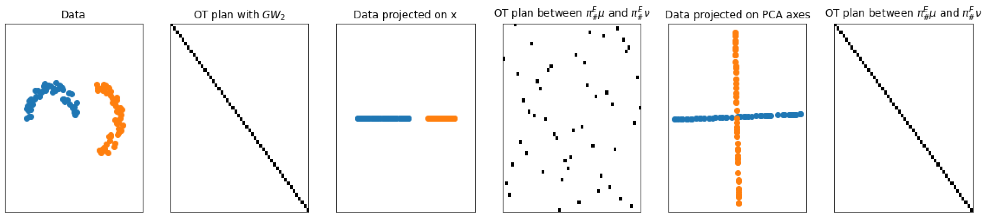
Algorithm 1 North-West corner rule $NW(a,b)$

$a\in {\Sigma }_n,b\in {\Sigma }_m$ while$i<=n$, $j<=m$do    ${\gamma }_{ij}=min\{a_i,b_j\}$    $a_i=a_i-{\gamma }_{ij}$    $b_j=b_j-{\gamma }_{ij}$    If $a_i=0$, $i=i+1$, if $b_j=0$, $j=j+1$ end while return$\gamma \in \mathsf{\Pi }(a,b)$

Proof. 

Let $\gamma \in \mathsf{\Pi }(a,b)$. Then:

$$\begin{array}{c}\hfill \sum _{ijkl}{(x_i{x}_k-y_j{y}_l)}^2{\gamma }_{ij}{\gamma }_{kl}=\sum _{ijkl}{\left(x_i{x}_k\right)}^2{\gamma }_{ij}{\gamma }_{kl}+\sum _{ijkl}{\left(y_j{y}_l\right)}^2{\gamma }_{ij}{\gamma }_{kl}-2\sum _{ijkl}{x}_i{x}_k{y}_j{y}_l{\gamma }_{ij}{\gamma }_{kl}\end{array}$$

However, ${\sum }_{ijkl}{\left(x_i{x}_k\right)}^2{\gamma }_{ij}{\gamma }_{kl}={\sum }_{ik}{\left(x_i{x}_k\right)}^2{a}_i{a}_k$, and ${\sum }_{ijkl}{\left(y_j{y}_l\right)}^2{\gamma }_{ij}{\gamma }_{kl}={\sum }_{jl}{\left(y_j{y}_l\right)}^2{b}_j{b}_l$, so this does not depend on $\gamma$. Moreover $2{\sum }_{ijkl}{x}_i{x}_k{y}_j{y}_l{\gamma }_{ij}{\gamma }_{kl}=2{\left({\sum }_{ij}{x}_i{y}_j{\gamma }_{ij}\right)}^2$. Hence, the problem (8) is equivalent to ${max}_{\gamma \in \mathsf{\Pi }(a,b)}{\left({\sum }_{ij}{x}_i{y}_j{\gamma }_{ij}\right)}^2$ (in terms of the OT plan), which is also equivalent to solving ${max}_{\gamma \in \mathsf{\Pi }(a,b)}\left|{\sum }_{ij}{x}_i{y}_j{\gamma }_{ij}\right|$ or equivalently:

$$\underset{\gamma \in \mathsf{\Pi }(a,b)}{max}\pm 1\sum _{ij}{x}_i{y}_j{\gamma }_{ij}$$

(9)

We have two cases to consider: If $\pm 1=1$, we have to solve $-{min}_{\gamma \in \mathsf{\Pi }(a,b)}{\sum }_{ij}(-x_i)y_j{\gamma }_{ij}$. Since the points are sorted, the matrix $c_{ij}=-x_i{y}_j$ satisfies the Monge property [33]:

$$\forall (i,j)\in \{1,\cdots ,n-1\}\times \{1,\cdots ,m-1\},c_{i,j}+c_{i+1,j+1}\le c_{i+1,j}+c_{i,j+1}$$

(10)

To see this, check that:

$$\begin{array}{cc}\hfill & (-x_i)y_j+(-x_{i+1})y_{j+1}-(-x_{i+1})y_j-(-x_i)y_{j+1}\hfill \\ \hfill & =(-x_i)(y_j-y_{j+1})+(-x_{i+1})(y_{j+1}-y_j)=(y_j-y_{j+1})(x_{i+1}-x_i)\le 0\hfill \end{array}$$

(11)

In this case, the North-West corner rule $NW(a,b)$ defined in Algorithm 1 is known to produce an optimal solution to the linear problem (9) [33]. If $\pm =-1$, then changing $x_i$ to $-x_i$ concludes. □

We emphasize that this result is novel and generalizes [12] in the sense that the distributions do not need to have uniform weights and the same number of points. I addition, Theorem 2 is not directly applicable to this setting since it requires having absolutely regular distributions, which is not the case here. Both results are, however, related, as the solution obtained by using the NW corner rule on the sorted samples is the same as that obtained by considering the coupling obtained from the quantile functions. The previous result could also be used to define tractable alternatives to GW in the same manner as the Sliced Gromov–Wasserstein [12].

3.5. Illustrations

We use the Python Optimal Transport (POT) library [34] to compute the different optimal transport problems involved in this illustration. We are interested here in solving a 3D mesh registration problem, which is a natural application of Gromov–Wasserstein [3] since it enjoys invariances with respect to isometries such as permutations and can also naturally exploit the topology of the meshes. For this purpose, we selected two base meshes from the Faust dataset [35], which provides ground truth correspondences between shapes. The information available from those meshes are geometrical (6890 vertices positions) and topological (mesh connectivity). These two meshes are represented, along with the visual results of the registration, in Figure 2. In order to visually depict the quality of the assignment induced by the transport map, we propagate through it a color code of the source vertices toward their associated counterpart vertices in the target mesh. Both the original color-coded source and the associated target ground truth are available on the first line of the illustration. To compute our method, we simply use as a natural subspace for both meshes the algebraic connectivity of the mesh’s topological information, also known as the Fiedler vector [36] (eigenvector associated to the second smallest eigenvalue of the un-normalized Laplacian matrix). Fiedler vectors are computed in practice using NetworkX [37] but could also be obtained by using power methods [38]. Reduced to a 1D optimal transport problem (8), we used the Proposition 5 to compute the optimal coupling in $O(n+m)$. Consequently, the computation time is very low ($\sim 5$ secs. on a standard laptop), and the associated matching is very good, with more than $98\%$ of correct assignments. We qualitatively compare this result to Gromov–Wasserstein mappings induced by different cost functions, in the second line of Figure 2: adjacency [39], weighted adjacency (weights are given by distances between vertices), heat kernel (derived from the un-normalized Laplacian) [40], and, finally, geodesic distances over the meshes. On average, computing the Gromov–Wasserstein mapping using POT took around 10 min of time. Both methods based on adjacency fail to recover a meaningful mapping. Heat kernel allows us to map continuous areas of the source mesh but fails in recovering a global structure. Finally, the geodesic distance gives a much more coherent mapping but has inverted left and right of the human figure. Notably, a significant extra computation time was induced by the computation of the geodesic distances ($\sim 1$ h/mesh using the NetworkX [37] shortest path procedure). As a conclusion, and despite the simplification of the original problem, our method performs best with a speed-up of two-orders of magnitude.

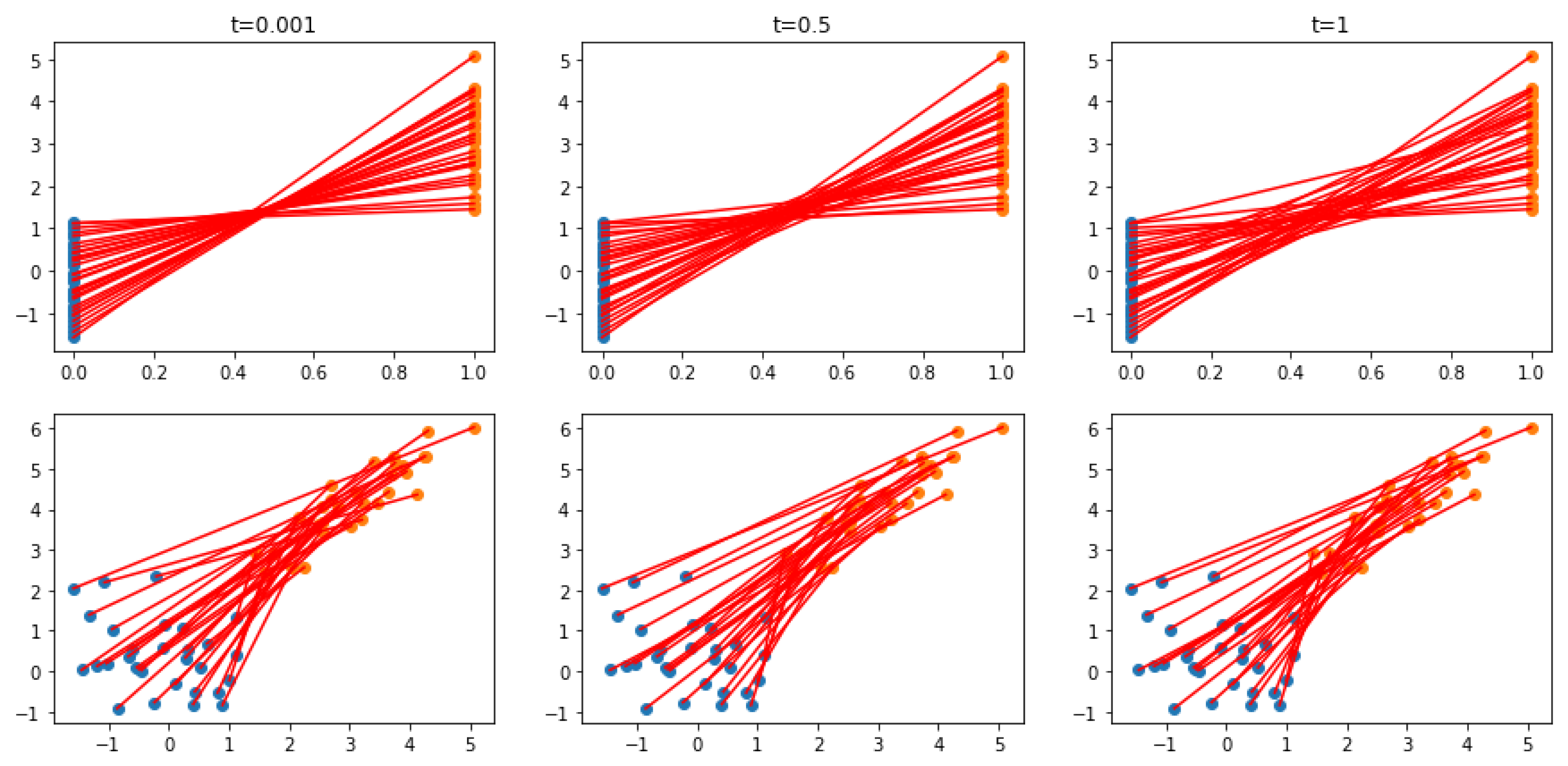
4. Triangular Coupling as Limit of Optimal Transport Plans for Quadratic Cost

Another interesting property derived in Muzellec and Cuturi [14] of the Monge–Knothe coupling is that it can be obtained as the limit of classic optimal transport plans, similar to Theorem 1, using a separable cost of the form:

$$c_t(x,y)={(x-y)}^T{P}_t(x-y)$$

with $P_t=V_E{V}_E^T+t{V}_{E^{\perp }}{V}_{E^{\perp }}^T$ and $(V_E,V_{E^{\perp }})$ as an orthonormal basis of ${\mathbb{R}}^p$.

However, this property is not valid for the classical Gromov–Wasserstein cost (e.g., $L(x,x^{\prime },y,y^{\prime })={(d_X{(x,x^{\prime })}^2-d_Y{(y,y^{\prime })}^2)}^2$ or $L(x,x^{\prime },y,y^{\prime })={({\langle x,x^{\prime }\rangle }_p-{\langle y,y^{\prime }\rangle }_q)}^2$) as the cost is not separable. Motivated by this question, we ask ourselves in the following if we can derive a quadratic optimal transport cost for which we would have this property.

Formally, we derive a new quadratic optimal transport problem using the Hadamard product. We show that this problem is well-defined and that it has interesting properties such as invariance with respect to axis. We also show that it can be related to a triangular coupling in a similar fashion than the classical optimal transport problem with the Knothe–Rosenblatt rearrangement.

4.1. Construction of the Hadamard–Wasserstein Problem

In this part, we define the “Hadamard–Wasserstein” problem between $\mu \in \mathcal{P}\left({\mathbb{R}}^d\right)$ and $\nu \in \mathcal{P}\left({\mathbb{R}}^d\right)$ as:

$${\mathcal{HW}}^2(\mu ,\nu )=\underset{\gamma \in \mathsf{\Pi }(\mu ,\nu )}{inf}\int \int {\parallel x\odot x^{\prime }-y\odot y^{\prime }\parallel }_2^2\mathrm{d}\gamma (x,y)\mathrm{d}\gamma (x^{\prime },y^{\prime }),$$

(12)

where ⊙ is the Hadamard product (element-wise product). This problem is different than the Gromov–Wasserstein problem in the sense that we do not compare intradistance anymore bur rather the Hadamard products between vectors of the two spaces (in the same fashion as the classical Wasserstein distance). Hence, we need the two measures to belong in the same Euclidean space. Let us note L as the cost defined as:

$$\forall x,x^{\prime },y,y^{\prime }\in {\mathbb{R}}^d,L(x,x^{\prime },y,y^{\prime })=\sum _{k=1}^d{(x_k{x}_k^{\prime }-y_k{y}_k^{\prime })}^2={\parallel x\odot x^{\prime }-y\odot y^{\prime }\parallel }_2^2.$$

(13)

We observe that it coincides with the inner-GW (4) loss in one dimension. Therefore, by Theorem 2, we know that we have a closed-form solution in 1D.

4.2. Properties

First, we derive some useful properties of (12) which are usual for the regular Gromov–Wasserstein problem. Formally, we show that the problem is well defined and that it is a pseudometric with invariances with respect to axes.

Proposition 6.

Let $\mu ,\nu \in \mathcal{P}\left({\mathbb{R}}^d\right)$.

• The problem (12) always admits a minimizer.
• $\mathcal{HW}$ is a pseudometric (i.e., it is symmetric, non-negative, $\mathcal{HW}(\mu ,\mu )=0$, and it satisfies the triangle inequality).
• $\mathcal{HW}$ is invariant to reflection with respect to axes.

Proof. 

Let $\mu ,\nu \in \mathcal{P}\left({\mathbb{R}}^d\right)$,

• $(x,x^{\prime })\mapsto x\odot x^{\prime }$ is a continuous map, therefore, L is less semi-continuous. Hence, by applying Lemma 2.2.1 of [26], we observe that $\gamma \mapsto \int \int L(x,x^{\prime },y,y^{\prime })\mathrm{d}\gamma (x,y)\mathrm{d}\gamma (x^{\prime },y^{\prime })$ is less semi-continuous for the weak convergence of measures.
  Now, as $\mathsf{\Pi }(\mu ,\nu )$ is a compact set (see the proof of Theorem 1.7 in [19] for the Polish space case and of Theorem 1.4 for the compact metric space) and $\gamma \mapsto \int \int L\mathrm{d}\gamma \mathrm{d}\gamma$ is less semi-continuous for the weak convergence, we can apply the Weierstrass theorem (Memo 2.2.1 in [26]), which states that (12) always admits a minimizer.
• See Theorem 16 in [25].
• For invariances, we first look at the properties that must be satisfied by T in order to have: $\forall x,x^{\prime },f(x,x^{\prime })=f(T\left(x\right),T\left(x^{\prime }\right))$ where $f:(x,x^{\prime })\mapsto x\odot x^{\prime }$.
  We find that $\forall x\in {\mathbb{R}}^d{,\forall 1\le i\le d,|\left[T\left(x\right)\right]}_i|=|x_i|$ because, denoting ${\left(e_i\right)}_{i=1}^d$ as the canonical basis, we have:

  $$x\odot e_i=T\left(x\right)\odot T\left(e_i\right),$$

  which implies that:

  $$x_i={\left[T\left(x\right)\right]}_i{\left[T\left(e_i\right)\right]}_i.$$
  However, $f(e_i,e_i)=f(T\left(e_i\right),T\left(e_i\right))$ implies ${\left[T\left(e_i\right)\right]}_i^2=1$, and therefore:

  $${|\left[T\left(x\right)\right]}_i|=|x_i|.$$
  If we take for T the reflection with respect to axis, then it satisfies $f(x,x^{\prime })=f(T\left(x\right),T\left(x^{\prime }\right))$ well. Moreover, it is a good equivalence relation, and therefore, we have a distance on the quotient space.

□

$\mathcal{HW}$ loses some properties compared to $GW$. Indeed, it is only invariant with respect to axes, and it can only compare measures lying in the same Euclidean space in order for the distance to be well defined. Nonetheless, we show in the following that we can derive some links with triangular couplings in the same way as the Wasserstein distance with KR.

Indeed, the cost L (13) is separable and reduces to the inner-GW loss in 1D, for which we have a closed-form solution. We can therefore define a degenerated version of it:

$$\begin{array}{cc}\hfill \forall x,x^{\prime },y,y^{\prime }\in {\mathbb{R}}^d,L_t(x,x^{\prime },y,y^{\prime })& =\sum _{k=1}^d\left(\prod _{i=1}^{k-1}{\lambda }_t^{\left(i\right)}\right){(x_k{x}_k^{\prime }-y_k{y}_k^{\prime })}^2\hfill \\ \hfill & ={(x\odot x^{\prime }-y\odot y^{\prime })}^T{A}_t(x\odot x^{\prime }-y\odot y^{\prime })\hfill \end{array}$$

(14)

with $A_t=\mathrm{diag}(1,{\lambda }_t^{\left(1\right)},{\lambda }_t^{\left(1\right)}{\lambda }_t^{\left(2\right)},\cdots ,{\prod }_{i=1}^{d-1}{\lambda }_t^{\left(i\right)})$, such as for all $t>0$, and for all $i\in \{1,\cdots ,d-1\}$, ${\lambda }_t^{\left(i\right)}>0$, and ${\lambda }_t^{\left(i\right)}\underset{t\to 0}{\to }0$. We denote ${\mathcal{HW}}_t$ the problem (12) with the degenerated cost (14). Therefore, we will be able to decompose the objective as:

$$\begin{array}{cc}\hfill & \int \int L_t(x,x^{\prime },y,y^{\prime })\mathrm{d}\gamma (x,y)\mathrm{d}\gamma (x^{\prime },y^{\prime })\hfill \\ & =\int \int {(x_1{x}_1^{\prime }-y_1{y}_1^{\prime })}^2\mathrm{d}\gamma (x,y)\mathrm{d}\gamma (x^{\prime },y^{\prime })\hfill \\ & +\int \int \sum _{k=2}^d\left(\prod _{i=1}^{k-1}{\lambda }_t^{\left(i\right)}\right){(x_k{x}_k^{\prime }-y_k{y}_k^{\prime })}^2\mathrm{d}\gamma (x,y)\mathrm{d}\gamma (x^{\prime },y^{\prime })\hfill \end{array}$$

and to use the same induction reasoning as [21].

Then, we can define a triangular coupling different from the Knothe–Rosenblatt rearrangement in the sense that each map will not be nondecreasing. Indeed, following Theorem 2, the solution of each 1D problem:

$$\underset{\gamma \in \mathsf{\Pi }(\mu ,\nu )}{argmin}\int \int {(x{x}^{\prime }-y{y}^{\prime })}^2\mathrm{d}\gamma (x,y)\mathrm{d}\gamma (x^{\prime },y^{\prime })$$

is either ${(Id\times T_{\mathrm{asc}})}_{\#}\mu$ or ${(Id\times T_{\mathrm{desc}})}_{\#}\mu$. Hence, at each step $k\ge 1$, if we disintegrate the joint law of the k first variables as ${\mu }^{1:k}={\mu }^{1:k-1}\otimes {\mu }^{k|1:k-1}$, the optimal transport map $T(·|x_1,\cdots ,x_{k-1})$ will be the solution of:

$$\underset{T\in \{T_{\mathrm{asc}},T_{\mathrm{desc}}\}}{argmin}\int \int {\left(x_k{x}_k^{\prime }-T\left(x_k\right)T\left(x_k^{\prime }\right)\right)}^2{\mu }^{k\mid 1:k-1}(\mathrm{d}{x}_k\mid x_{1:k-1}){\mu }^{k\mid 1:k-1}(\mathrm{d}{x}_k^{\prime }\mid x_{1:k-1}^{\prime }).$$

We now state the main theorem, where we show that the limit of the OT plans obtained with the degenerated cost will be the triangular coupling we just defined.

Theorem 3.

Let μ and ν be two absolutely continuous measures on ${\mathbb{R}}^d$ such that ${\int \parallel x\parallel }_2^4\mu \left(\mathrm{d}x\right)<+\infty$, ${\int \parallel y\parallel }_2^4\nu \left(\mathrm{d}y\right)<+\infty$ and with compact support. Let ${\gamma }_t$ be an optimal transport plan for ${\mathcal{HW}}_t$, let $T_K$ be the alternate Knothe–Rosenblatt map between μ and ν as defined in the last paragraph, and let ${\gamma }_K={(Id\times T_K)}_{\#}\mu$ be the associated transport plan. Then, we have ${\gamma }_t\underset{t\to 0}{\overset{\mathcal{D}}{\to }}{\gamma }_K$. Moreover, if ${\gamma }_t$ are induced by transport maps $T_t$, then $T_t\underset{t\to 0}{\overset{L^2\left(\mu \right)}{\to }}{T}_K$.

Proof. 

See Appendix B.2. □

However, we cannot extend this Theorem to the subspace detour approach. Indeed, by choosing $A_t=V_E{V}_E^T+t{V}_{E^{\perp }}{V}_{E^{\perp }}^T$ with $(V_E,V_{E^{\perp }})$ an orthonormal basis of ${\mathbb{R}}^d$, then we project $x\odot x^{\prime }-y\odot y^{\prime }$ on E (respectively on $E^{\perp }$), which is generally different from $x_E\odot x_E^{\prime }-y_E\odot y_E^{\prime }$ (respectively $x_{E^{\perp }}\odot x_{E^{\perp }}^{\prime }-y_{E^{\perp }}\odot y_{E^{\perp }}^{\prime }$).

4.3. Solving Hadamard–Wasserstein in the Discrete Setting

In this part, we derive formulas to solve numerically $\mathcal{HW}$ (12). Let $x_1,\cdots ,x_n\in {\mathbb{R}}^d$, $y_1,\cdots ,y_m\in {\mathbb{R}}^d$, $\alpha \in {\Sigma }_n$, $\beta \in {\Sigma }_m$, $p={\sum }_{i=1}^n{\alpha }_i{\delta }_{x_i}$ and $q={\sum }_{j=1}^m{\beta }_j{\delta }_{y_j}$ two discrete measures in ${\mathbb{R}}^d$. The Hadamard Wasserstein problem (12) becomes in the discrete setting:

$$\begin{array}{cc}\hfill {\mathcal{HW}}^2(p,q)& =\underset{\gamma \in \mathsf{\Pi }(p,q)}{inf}\sum _{i,j}\sum _{k,\ell }{\parallel x_i\odot x_k-y_j\odot y_{\ell }\parallel }_2^2{\gamma }_{i,j}{\gamma }_{k,\ell }\hfill \\ \hfill & =\underset{\gamma \in \mathsf{\Pi }(p,q)}{inf}\mathcal{E}\left(\gamma \right)\hfill \end{array}$$

with $\mathcal{E}\left(\gamma \right)={\sum }_{i,j}{\sum }_{k,\ell }{\parallel x_i\odot x_k-y_j\odot y_{\ell }\parallel }_2^2{\gamma }_{i,j}{\gamma }_{k,\ell }$. As denoted in [9], if we note:

$${\mathcal{L}}_{i,j,k,\ell }={\parallel x_i\odot x_k-y_j\odot y_{\ell }\parallel }_2^2,$$

then we have:

$$\mathcal{E}\left(\gamma \right)=\langle \mathcal{L}\otimes \gamma ,\gamma \rangle ,$$

where ⊗ is defined as:

$$\mathcal{L}\otimes \gamma ={\left(\sum _{k,\ell }{\mathcal{L}}_{i,j,k,\ell }{\gamma }_{k,\ell }\right)}_{i,j}\in {\mathbb{R}}^{n\times m}.$$

We show in the next proposition a decomposition of $\mathcal{L}\otimes \gamma$, which allows us to compute this tensor product more efficiently.

Proposition 7.

Let $\gamma \in \mathsf{\Pi }(p,q)=\{M\in {\left({\mathbb{R}}_{+}\right)}^{n\times m},M{𝟙}_m=p,M^T{𝟙}_n=q\}$, where ${𝟙}_n={(1,\cdots ,1)}^T\in {\mathbb{R}}^n$. Let us note $X={(x_i\odot x_k)}_{i,k}\in {\mathbb{R}}^{n\times n\times d}$, $Y={(y_j\odot y_{\ell })}_{j,\ell }\in {\mathbb{R}}^{m\times m\times d}$, $X^{\left(2\right)}=(\parallel X_{i,k}{{\parallel }_2^2)}_{i,k}\in {\mathbb{R}}^{n\times n}$, $Y^{\left(2\right)}=(\parallel Y_{j,l}{{\parallel }_2^2)}_{j,l}\in {\mathbb{R}}^{m\times m}$, and $\forall t\in \{1,\cdots ,d\},X_t={\left(X_{i,k,t}\right)}_{i,k}\in {\mathbb{R}}^{n\times n}$ and $Y_t={\left(Y_{j,\ell ,t}\right)}_{j,\ell }\in {\mathbb{R}}^{m\times m}$. Then:

$$\mathcal{L}\otimes \gamma =X^{\left(2\right)}p{𝟙}_m^T+{𝟙}_n{q}^T{\left(Y^{\left(2\right)}\right)}^T-2\sum _{t=1}^d{X}_t\gamma Y_t^T.$$

Proof. 

First, we can start by writing:

$$\begin{array}{cc}\hfill {\mathcal{L}}_{i,j,k,\ell }& =\parallel x_i\odot x_k-y_j\odot y_{\ell }{\parallel }_2^2\hfill \\ \hfill & =\parallel X_{i,k}-Y_{j,\ell }{\parallel }_2^2\hfill \\ \hfill & =\parallel X_{i,k}{\parallel }_2^2+{\parallel Y_{j,\ell }\parallel }_2^2-2\langle X_{i,k},Y_{j,\ell }\rangle \hfill \\ \hfill & ={[X^{\left(2\right)}]}_{i,k}+{[Y^{\left(2\right)}]}_{j,\ell }-2\langle X_{i,k},Y_{j,\ell }\rangle .\hfill \end{array}$$

We cannot directly apply proposition 1 from [9] (as the third term is a scalar product), but by performing the same type of computation, we obtain:

$$\mathcal{L}\otimes \gamma =A+B+C$$

with

$$A_{i,j}=\sum _{k,\ell }{[X^{\left(2\right)}]}_{i,k}{\gamma }_{k,\ell }=\sum _k{[X^{\left(2\right)}]}_{i,k}\sum _{\ell }{\gamma }_{k,\ell }=\sum _k{[X^{\left(2\right)}]}_{i,k}{\left[\gamma {𝟙}_m\right]}_{k,1}={[X^{\left(2\right)}\gamma {𝟙}_m]}_{i,1}={[X^{\left(2\right)}p]}_{i,1}$$

$$B_{i,j}=\sum _{k,\ell }{[Y^{\left(2\right)}]}_{j,\ell }{\gamma }_{k,\ell }=\sum _{\ell }{[Y^{\left(2\right)}]}_{j,\ell }\sum _k{\gamma }_{k,\ell }=\sum _{\ell }{[Y^{\left(2\right)}]}_{j,\ell }{\left[{\gamma }^T{𝟙}_n\right]}_{\ell ,1}={[Y^{\left(2\right)}{\gamma }^T{𝟙}_n]}_{j,1}={[Y^{\left(2\right)}q]}_{j,1}$$

and

$$\begin{array}{cc}\hfill C_{i,j}=-2\sum _{k,\ell }\langle X_{i,k},Y_{j,\ell }\rangle {\gamma }_{k,\ell }& =-2\sum _{k,\ell }\sum _{t=1}^d{X}_{i,k,t}{Y}_{j,\ell ,t}{\gamma }_{k,\ell }\hfill \\ \hfill & =-2\sum _{t=1}^d\sum _k{\left[X_t\right]}_{i,k}\sum _{\ell }{\left[Y_t\right]}_{j,\ell }{\gamma }_{\ell ,k}^T\hfill \\ \hfill & =-2\sum _{t=1}^d\sum _k{\left[X_t\right]}_{i,k}{\left[Y_t{\gamma }^T\right]}_{j,k}\hfill \\ \hfill & =-2\sum _{t=1}^d{\left[X_t{\left(Y_t{\gamma }^T\right)}^T\right]}_{i,j}.\hfill \end{array}$$

Finally, we have:

$$\mathcal{L}\otimes \gamma =X^{\left(2\right)}p{𝟙}_m^T+{𝟙}_n{q}^T{\left(Y^{\left(2\right)}\right)}^T-2\sum _{t=1}^d{X}_t\gamma Y_t^T.$$

□

From this decomposition, we can compute the tensor product $\mathcal{L}\otimes \gamma$ with a complexity of $O\left(d(n^{2}m+m^{2}n)\right)$ using only multiplications of matrices (instead of $O\left(d{n}^2{m}^2\right)$ for a naive computation).

Remark 1.

For the degenerated cost function (14), we just need to replace X and Y by $\widetilde{X_t}=A_t^{\frac{1}{2}}X$ and $\widetilde{Y_t}=A_t^{\frac{1}{2}}Y$ in the previous proposition.

To solve this problem numerically, we can use the conditional gradient algorithm (Algorithm 2 in [41]). This algorithm only requires to compute the gradient:

$$\nabla \mathcal{E}\left(\gamma \right)=2(A+B+C)=2(\mathcal{L}\otimes \gamma )$$

at each step and a classical OT problem. This algorithm is more efficient than solving the quadratic problem directly. Moreover, while it is a non-convex problem, it actually converges to a local stationary point [42].

On Figure 3, we generated 30 points of 2 Gaussian distributions, and computed the optimal coupling of ${\mathcal{HW}}_t$ for several t. These points have the same uniform weight. We plot the couplings between the points on the second row, and between the projected points on their first coordinate on the first row. Note that for discrete points, the Knothe–Rosenblatt coupling amounts to sorting the points with respect to the first coordinate if there is no ambiguity (i.e., $x_1^{\left(1\right)}<\cdots <x_n^{\left(1\right)}$) as it comes back to perform the optimal transport in one dimension [43] (Remark 2.28). For our cost, the optimal coupling in 1D can either be the increasing or the decreasing rearrangement. We observe on the first row of Figure 3 that the optimal coupling when t is close to 0 corresponds to the decreasing rearrangement, which corresponds well to the alternate Knothe–Rosenblatt map we defined in Section 4.2. It underlines the results provided in Theorem 3.

5. Discussion

We proposed in this work to extend the subspace detour approach to different subspaces, and to other optimal transport costs such as Gromov–Wasserstein. Being able to project on different subspaces can be useful when the data are not aligned and do not share the same axes of interest, as well as when we are working between different metric spaces as it is the case, for example, with graphs. However, a question that arises is how to choose these subspaces. Since the method is mostly interesting when we choose one-dimensional subspaces, we proposed to use a PCA and to project on the first directions for data embedded in Euclidean spaces. For more complicated data such as graphs, we projected onto the Fiedler vector and obtained good results in an efficient way on a 3D mesh registration problem. More generally, Muzellec and Cuturi [14] proposed to perform a gradient descent on the loss with respect to orthonormal matrices. This approach is non-convex and is only guaranteed to converge to a local minimum. Designing such an algorithm, which would minimize alternatively between two transformations in the Stiefel manifold, is left for future works.

The subspace detour approach for transport problem is meaningful whenever one can identify subspaces that gather most of the information from the original distributions, while making the estimate more robust and with a better sample complexity as far as dimensions are lower. On the computational complexity side, and when we have only access to discrete data, the subspace detour approach brings better computational complexity solely when the subspaces are chosen as one dimensional. Indeed, otherwise, we have the same complexity for solving the subspace detour and solving the OT problem directly (since the complexity only depends on the number of samples). In this case, the 1D projection often gives distinct values for all the samples (for continuous valued data) and hence the Monge–Knothe coupling is exactly the coupling in 1D. As such, information is lost on the orthogonal spaces. It can be artificially recovered by quantizing the 1D values (as experimented in practice in [14]), but the added value is not clear and deserves broader studies. If given absolutely continuous distributions wrt. the Lebesgue measure, however, this limit does not exist but comes with the extra cost of being able to compute efficiently the projected measure onto the subspace, which might require discretization of the space and is therefore not practical in high dimensions.

We also proposed a new quadratic cost $\mathcal{HW}$ that we call Hadamard–Wasserstein, which allows us to define a degenerated cost for which the optimal transport plan converges to a triangular coupling. However, this cost loses many properties compared to $W_2$ or $GW$, for which we are inclined to use these problems. Indeed, while $\mathcal{HW}$ is a quadratic cost, it uses a Euclidean norm between the Hadamard product of vectors and requires the two spaces to be the same (in order to have the distance well defined). A work around in the case $X={\mathbb{R}}^p$ and $Y={\mathbb{R}}^q$ with $p\le q$ would be to “lift” the vectors in ${\mathbb{R}}^p$ into vectors in ${\mathbb{R}}^q$ with padding as it is proposed in [12] or to project the vectors in ${\mathbb{R}}^q$ on ${\mathbb{R}}^p$ as in [6]. Yet, for some applications where only the distance/similarity matrices are available, a different strategy still needs to be found. Another concern is the limited invariance properties (only with respect to axial symmetry symmetry in our case). Nevertheless, we expect that such a cost can be of interest in cases where invariance to symmetry is a desired property, such as in [44].

References

1. Arjovsky, M.; Chintala, S.; Bottou, L. Wasserstein generative adversarial networks. In Proceedings of the International Conference on Machine Learning, PMLR, Sydney, Australia, 6–11 August 2017; pp. 214–223. [Google Scholar]
2. Courty, N.; Flamary, R.; Tuia, D.; Rakotomamonjy, A. Optimal transport for domain adaptation. IEEE Trans. Pattern Anal. Mach. Intell. 2016, 39, 1853–1865. [Google Scholar] [CrossRef] [PubMed]
3. Mémoli, F. Gromov–Wasserstein distances and the metric approach to object matching. Found. Comput. Math. 2011, 11, 417–487. [Google Scholar] [CrossRef]
4. Chowdhury, S.; Miller, D.; Needham, T. Quantized Gromov–Wasserstein. In Proceedings of the Machine Learning and Knowledge Discovery in Databases, Research Track—European Conference, ECML PKDD 2021, Bilbao, Spain, 13–17 September 2021; Proceedings, Part III. Oliver, N., Pérez-Cruz, F., Kramer, S., Read, J., Lozano, J.A., Eds.; Springer: Berlin/Heidelberg, Germany, 2021; Volume 12977, pp. 811–827. [Google Scholar] [CrossRef]
5. Alvarez-Melis, D.; Jegelka, S.; Jaakkola, T.S. Towards optimal transport with global invariances. In Proceedings of the The 22nd International Conference on Artificial Intelligence and Statistics, PMLR, Naha, Japan, 16–18 April 2019; pp. 1870–1879. [Google Scholar]
6. Cai, Y.; Lim, L.H. Distances between probability distributions of different dimensions. arXiv 2020, arXiv:2011.00629. [Google Scholar]
7. Mémoli, F. On the use of Gromov-Hausdorff Distances for Shape Comparison. In Proceedings of the 4th Symposium on Point Based Graphics, PBG@Eurographics 2007, Prague, Czech Republic, 2–3 September 2007; Botsch, M., Pajarola, R., Chen, B., Zwicker, M., Eds.; Eurographics Association: Switzerland, Geneve, 2007; pp. 81–90. [Google Scholar] [CrossRef]
8. Sturm, K.T. The space of spaces: Curvature bounds and gradient flows on the space of metric measure spaces. arXiv 2012, arXiv:1208.0434. [Google Scholar]
9. Peyré, G.; Cuturi, M.; Solomon, J. Gromov–Wasserstein averaging of kernel and distance matrices. In Proceedings of the International Conference on Machine Learning, PMLR, New York, NY, USA, 19–24 June 2016; pp. 2664–2672. [Google Scholar]
10. Cuturi, M. Sinkhorn distances: Lightspeed computation of optimal transport. Adv. Neural Inf. Process. Syst. 2013, 26, 2292–2300. [Google Scholar]
11. Scetbon, M.; Peyré, G.; Cuturi, M. Linear-Time Gromov Wasserstein Distances using Low Rank Couplings and Costs. arXiv 2021, arXiv:2106.01128. [Google Scholar]
12. Vayer, T.; Flamary, R.; Courty, N.; Tavenard, R.; Chapel, L. Sliced Gromov–Wasserstein. Adv. Neural Inf. Process. Syst. 2019, 32, 14753–14763. [Google Scholar]
13. Fatras, K.; Zine, Y.; Majewski, S.; Flamary, R.; Gribonval, R.; Courty, N. Minibatch optimal transport distances; analysis and applications. arXiv 2021, arXiv:2101.01792. [Google Scholar]
14. Muzellec, B.; Cuturi, M. Subspace Detours: Building Transport Plans that are Optimal on Subspace Projections. In Proceedings of the Advances in Neural Information Processing Systems 32: Annual Conference on Neural Information Processing Systems 2019, NeurIPS 2019, Vancouver, BC, Canada, 8–14 December 2019; Wallach, H.M., Larochelle, H., Beygelzimer, A., d’Alché-Buc, F., Fox, E.B., Garnett, R., Eds.; 2019; pp. 6914–6925. [Google Scholar]
15. Bogachev, V.I.; Kolesnikov, A.V.; Medvedev, K.V. Triangular transformations of measures. Sb. Math. 2005, 196, 309. [Google Scholar] [CrossRef] [Green Version]
16. Knothe, H. Contributions to the theory of convex bodies. Mich. Math. J. 1957, 4, 39–52. [Google Scholar] [CrossRef]
17. Rosenblatt, M. Remarks on a multivariate transformation. Ann. Math. Stat. 1952, 23, 470–472. [Google Scholar] [CrossRef]
18. Villani, C. Optimal Transport: Old and New; Springer Science & Business Media: Berlin/Heidelberg, Germany, 2008; Volume 338. [Google Scholar]
19. Santambrogio, F. Optimal transport for applied mathematicians. Birkäuser NY 2015, 55, 94. [Google Scholar]
20. Jaini, P.; Selby, K.A.; Yu, Y. Sum-of-Squares Polynomial Flow. In Proceedings of the 36th International Conference on Machine Learning, PMLR, Long Beach, CA, USA, 9–15 June 2019; pp. 3009–3018. [Google Scholar]
21. Carlier, G.; Galichon, A.; Santambrogio, F. From Knothe’s transport to Brenier’s map and a continuation method for optimal transport. SIAM J. Math. Anal. 2010, 41, 2554–2576. [Google Scholar] [CrossRef] [Green Version]
22. Bonnotte, N. Unidimensional and Evolution Methods for Optimal Transportation. Ph.D. Thesis, Université Paris-Sud, Paris, France, 2013. [Google Scholar]
23. Ambrosio, L.; Gigli, N.; Savaré, G. Gradient Flows: In Metric Spaces and in the Space of Probability Measures; Springer Science & Business Media: Berlin/Heidelberg, Germany, 2008. [Google Scholar]
24. Niles-Weed, J.; Rigollet, P. Estimation of wasserstein distances in the spiked transport model. arXiv 2019, arXiv:1909.07513. [Google Scholar]
25. Chowdhury, S.; Mémoli, F. The gromov–wasserstein distance between networks and stable network invariants. Inf. Inference A J. IMA 2019, 8, 757–787. [Google Scholar] [CrossRef] [Green Version]
26. Vayer, T. A Contribution to Optimal Transport on Incomparable Spaces. Ph.D. Thesis, Université de Bretagne Sud, Vannes, France, 2020. [Google Scholar]
27. Paty, F.P.; Cuturi, M. Subspace robust wasserstein distances. In Proceedings of the 36th International Conference on Machine Learning, PMLR, Long Beach, CA, USA, 9–15 June 2019; pp. 5072–5081. [Google Scholar]
28. Rasmussen, C.E. Gaussian processes in machine learning. In Summer School on Machine Learning; Springer: Berlin/Heidelberg, Germany, 2003; pp. 63–71. [Google Scholar]
29. Von Mises, R. Mathematical Theory of Probability and Statistics; Academic Press: Cambridge, MA, USA, 1964. [Google Scholar]
30. Salmona, A.; Delon, J.; Desolneux, A. Gromov–Wasserstein Distances between Gaussian Distributions. arXiv 2021, arXiv:2104.07970. [Google Scholar]
31. Weed, J.; Bach, F. Sharp asymptotic and finite-sample rates of convergence of empirical measures in Wasserstein distance. Bernoulli 2019, 25, 2620–2648. [Google Scholar] [CrossRef] [Green Version]
32. Lin, T.; Zheng, Z.; Chen, E.; Cuturi, M.; Jordan, M. On projection robust optimal transport: Sample complexity and model misspecification. In Proceedings of the International Conference on Artificial Intelligence and Statistics, PMLR, Virtual, 13–15 April 2021; pp. 262–270. [Google Scholar]
33. Burkard, R.E.; Klinz, B.; Rudolf, R. Perspectives of Monge Properties in Optimization. Discret. Appl. Math. 1996, 70, 95–161. [Google Scholar] [CrossRef] [Green Version]
34. Flamary, R.; Courty, N.; Gramfort, A.; Alaya, M.Z.; Boisbunon, A.; Chambon, S.; Chapel, L.; Corenflos, A.; Fatras, K.; Fournier, N.; et al. POT: Python Optimal Transport. J. Mach. Learn. Res. 2021, 22, 1–8. [Google Scholar]
35. Bogo, F.; Romero, J.; Loper, M.; Black, M.J. FAUST: Dataset and evaluation for 3D mesh registration. In Proceedings of the IEEE Conference on Computer Vision and Pattern Recognition, Columbus, OH, USA, 23–28 June 2014; pp. 3794–3801. [Google Scholar]
36. Fiedler, M. Algebraic connectivity of graphs. Czechoslov. Math. J. 1973, 23, 298–305. [Google Scholar] [CrossRef]
37. Hagberg, A.; Swart, P.; Chult, D.S. Exploring Network Structure, Dynamics, and Function Using NetworkX; Technical Report; Los Alamos National Lab. (LANL): Los Alamos, NM, USA, 2008.
38. Wu, J.P.; Song, J.Q.; Zhang, W.M. An efficient and accurate method to compute the Fiedler vector based on Householder deflation and inverse power iteration. J. Comput. Appl. Math. 2014, 269, 101–108. [Google Scholar] [CrossRef]
39. Xu, H.; Luo, D.; Carin, L. Scalable Gromov–Wasserstein learning for graph partitioning and matching. Adv. Neural Inf. Process. Syst. 2019, 32, 3052–3062. [Google Scholar]
40. Chowdhury, S.; Needham, T. Generalized spectral clustering via Gromov–Wasserstein learning. In Proceedings of the International Conference on Artificial Intelligence and Statistics, PMLR, Virtual, 13–15 April 2021; pp. 712–720. [Google Scholar]
41. Vayer, T.; Courty, N.; Tavenard, R.; Flamary, R. Optimal transport for structured data with application on graphs. In Proceedings of the 36th International Conference on Machine Learning, PMLR, Long Beach, CA, USA, 9–15 June 2019; pp. 6275–6284. [Google Scholar]
42. Lacoste-Julien, S. Convergence rate of frank-wolfe for non-convex objectives. arXiv 2016, arXiv:1607.00345. [Google Scholar]
43. Peyré, G.; Cuturi, M. Computational optimal transport: With applications to data science. Found. Trends® Mach. Learn. 2019, 11, 355–607. [Google Scholar] [CrossRef]
44. Nagar, R.; Raman, S. Detecting approximate reflection symmetry in a point set using optimization on manifold. IEEE Trans. Signal Process. 2019, 67, 1582–1595. [Google Scholar] [CrossRef] [Green Version]
45. Billingsley, P. Convergence of Probability Measures; John Wiley & Sons: Hoboken, NJ, USA, 2013. [Google Scholar]
Figure 1. From left to right: Data (moons); OT plan obtained with GW for c ( x , x ) = x x 2 2 ; Data projected on the first axis; OT plan obtained between the projected measures; Data projected on their first PCA component; OT plan obtained between the the projected measures.
Algorithms 14 00366 g001
Figure 2. Three-dimensional mesh registration. (First row) source and target meshes, color code of the source, ground truth color code on the target, result of subspace detour using Fiedler vectors as subspace. (Second row) After recalling the expected ground truth for ease of comparison, we present results of different Gromov–Wasserstein mappings obtained with metrics based on adjacency, heat kernel, and geodesic distances.
Algorithms 14 00366 g002
Figure 3. Degenerated coupling. On the first row, the points are projected on their first coordinate and we plot the optimal coupling. On the second row, we plot the optimal coupling between the original points.
Algorithms 14 00366 g003
Publisher’s Note: MDPI stays neutral with regard to jurisdictional claims in published maps and institutional affiliations.