
Selection of Key Frames for 3D Reconstruction in Real Time

Abstract
:1. Introduction
2. Related Work
3. Materials and Methods
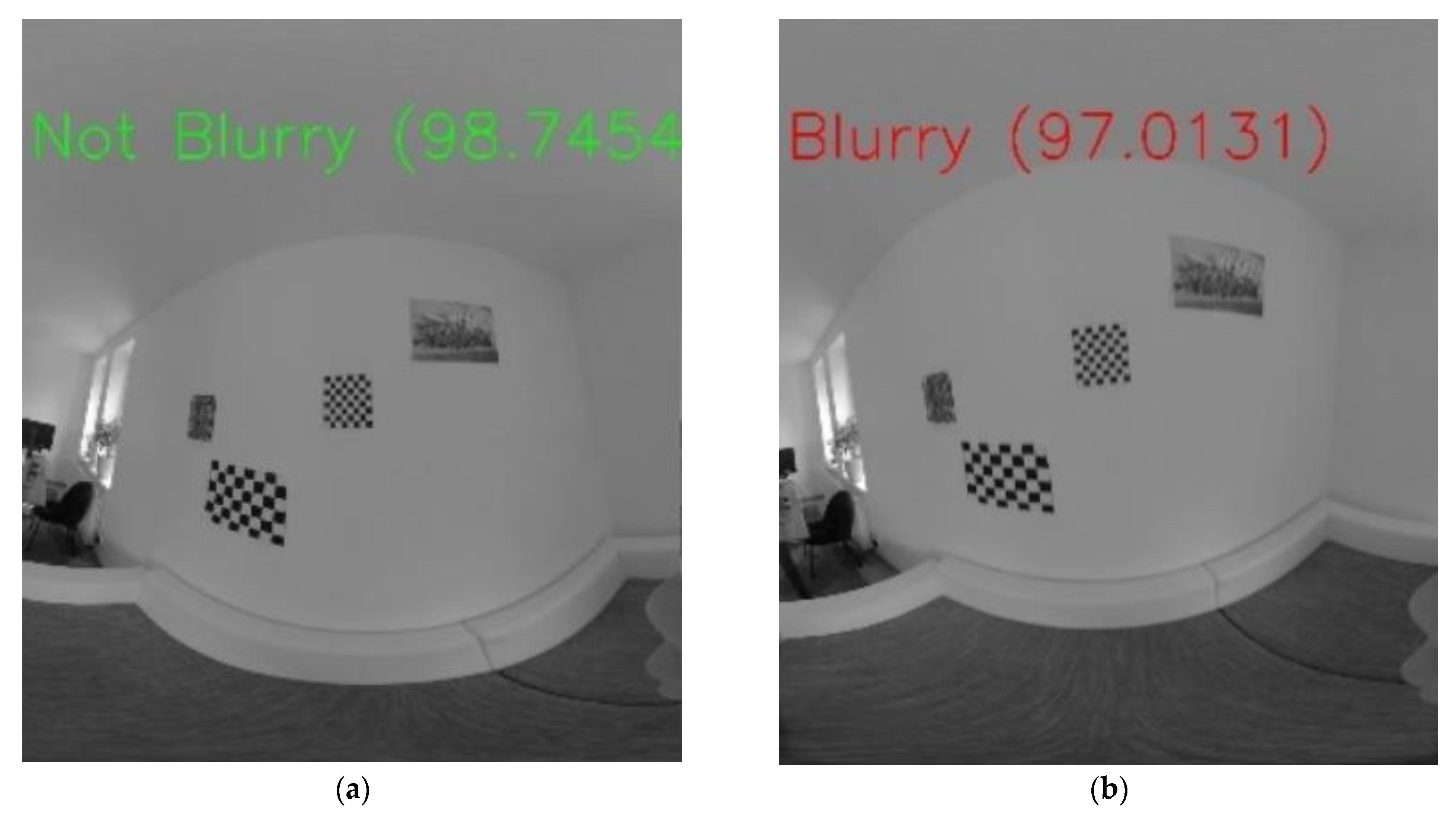
3.1. Quality Requirements
Quality Threshold
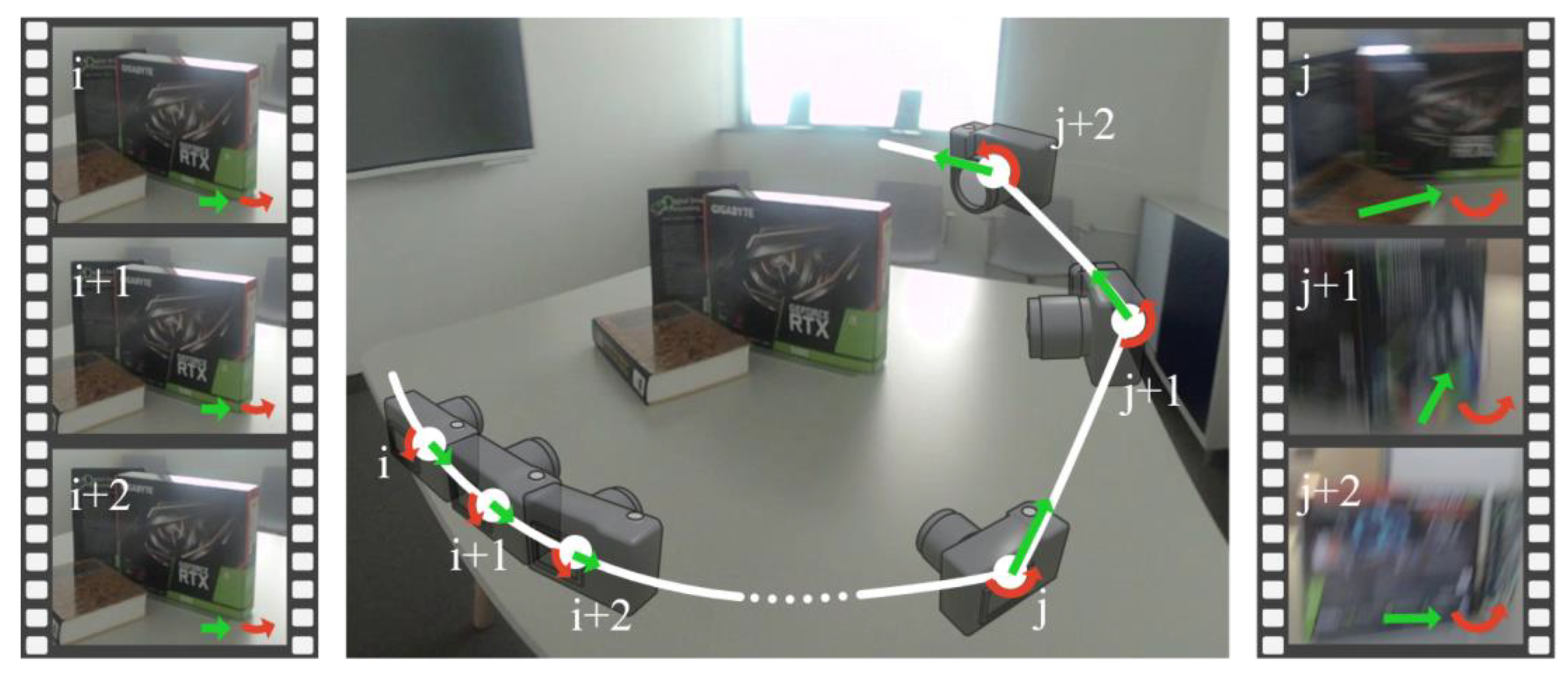
3.2. Motion Requirements
Motion Threshold
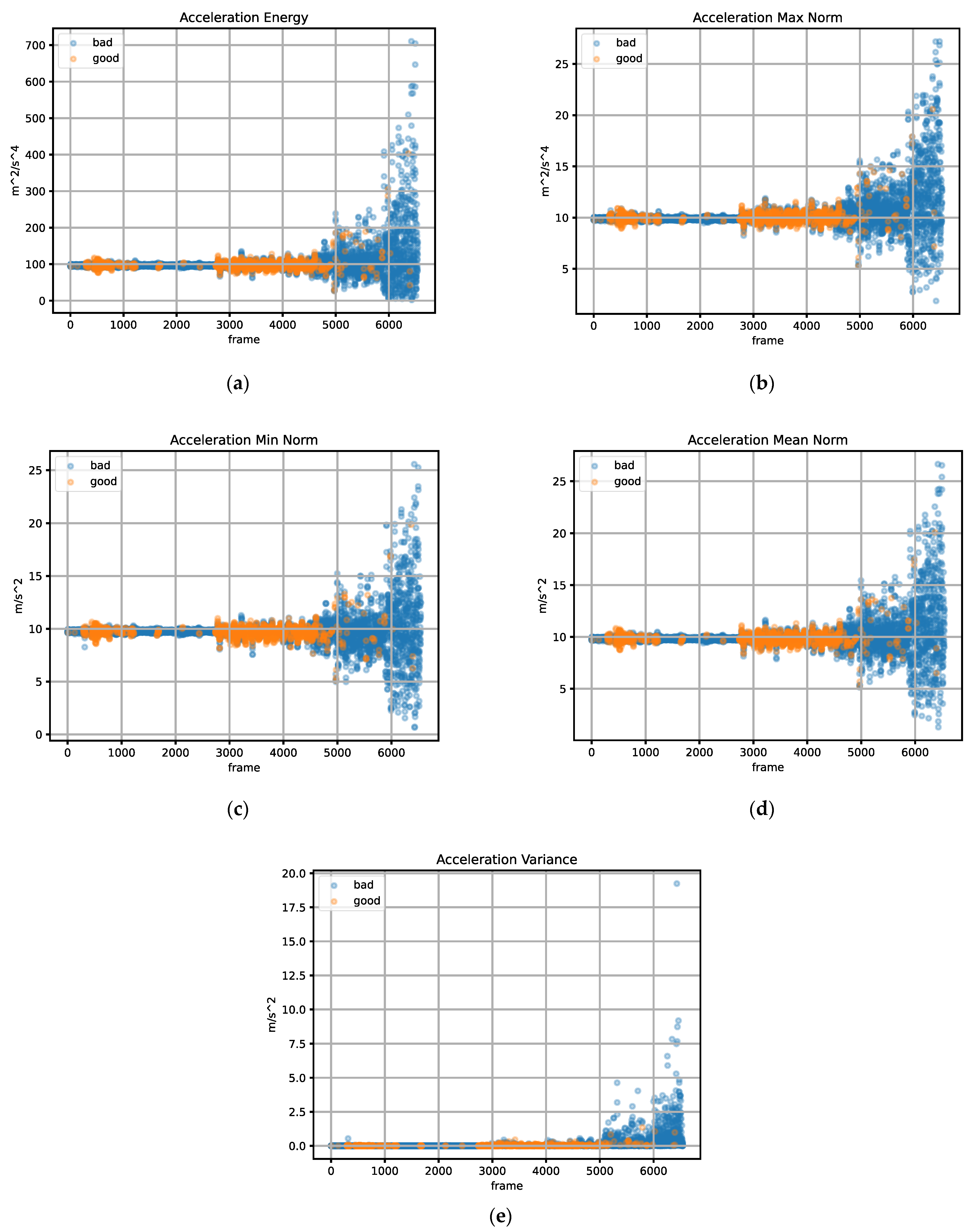
3.3. Feature Selection
- Signal Energy.
- 2.
- Mean Signal Norm.
- 3.
- Min Signal Norm.
- 4.
- Max Signal Norm.
- 5.
- Signal Variance.
4. Results and Discussion
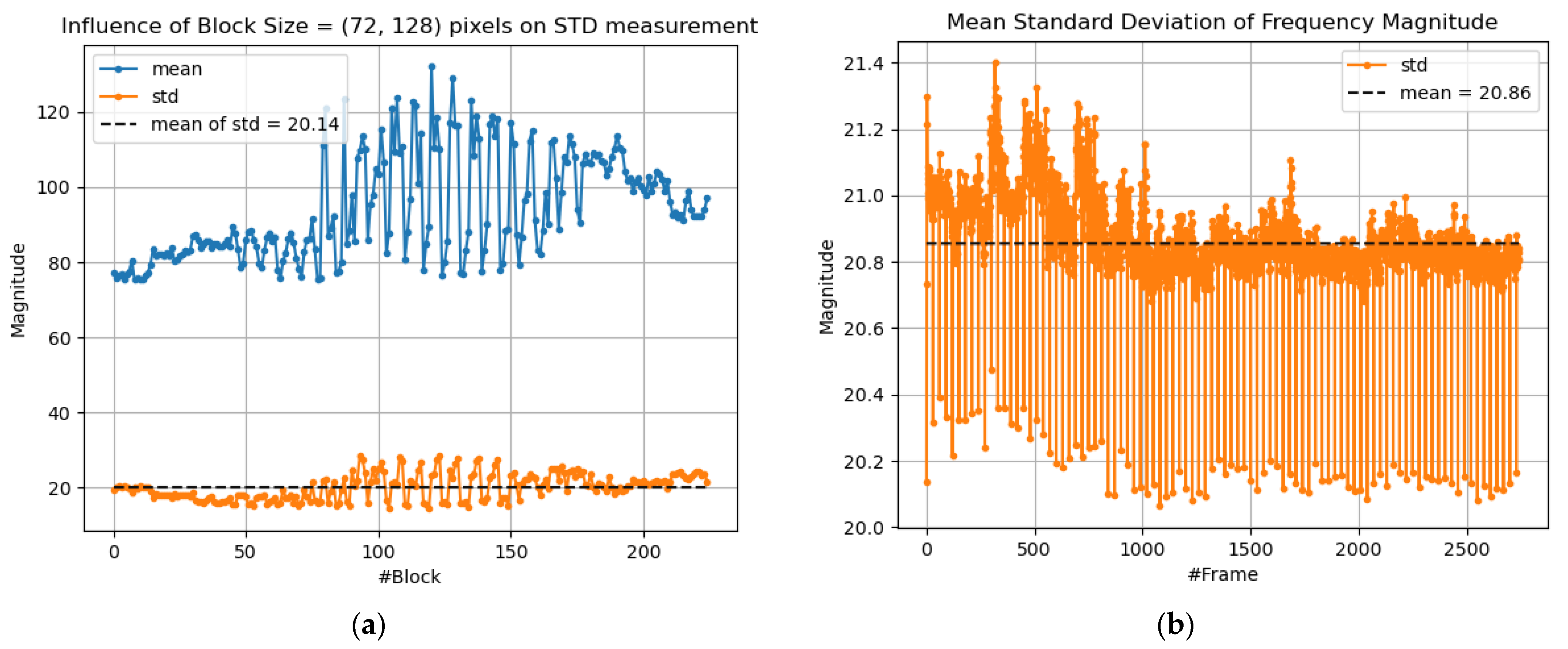
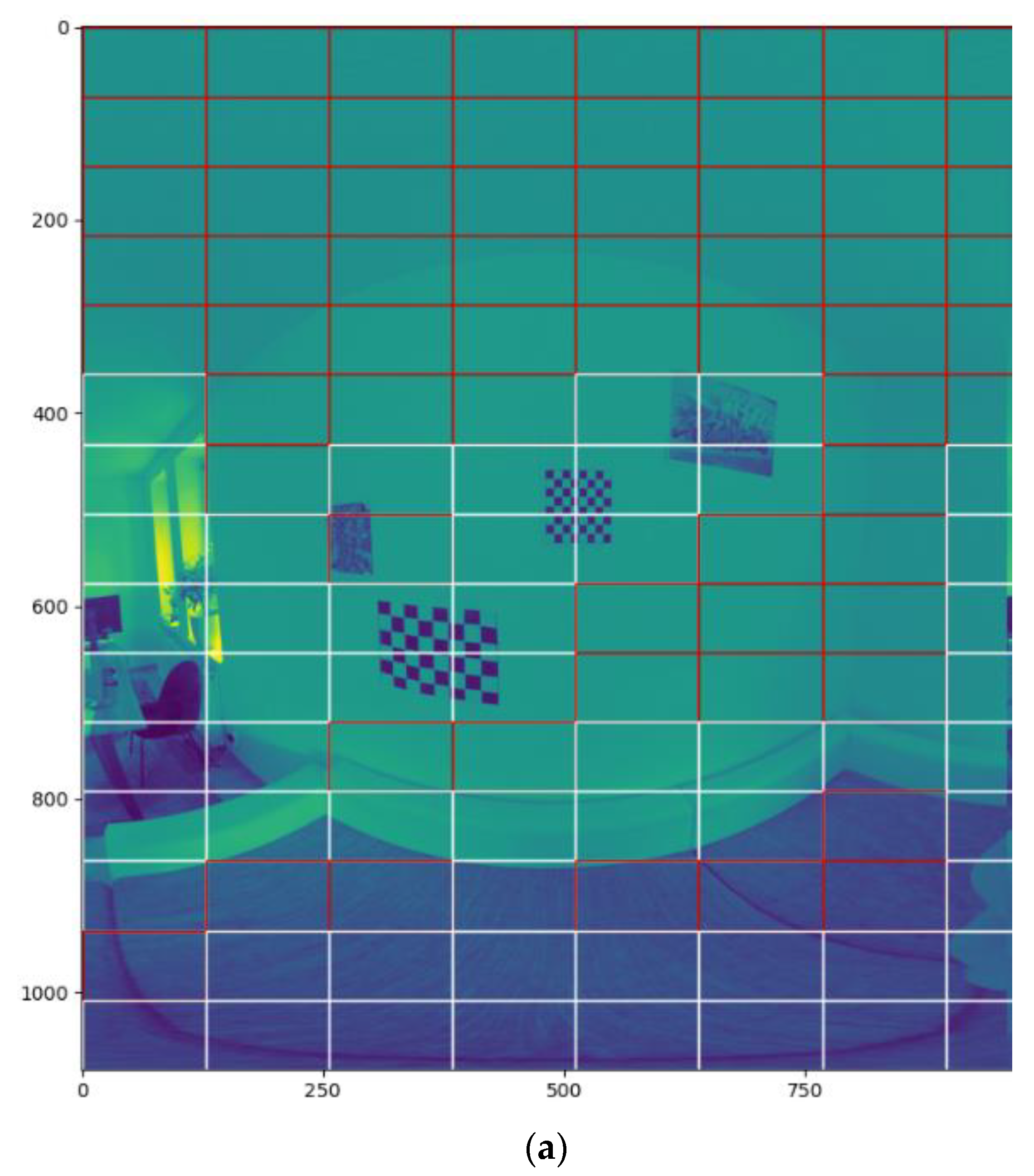
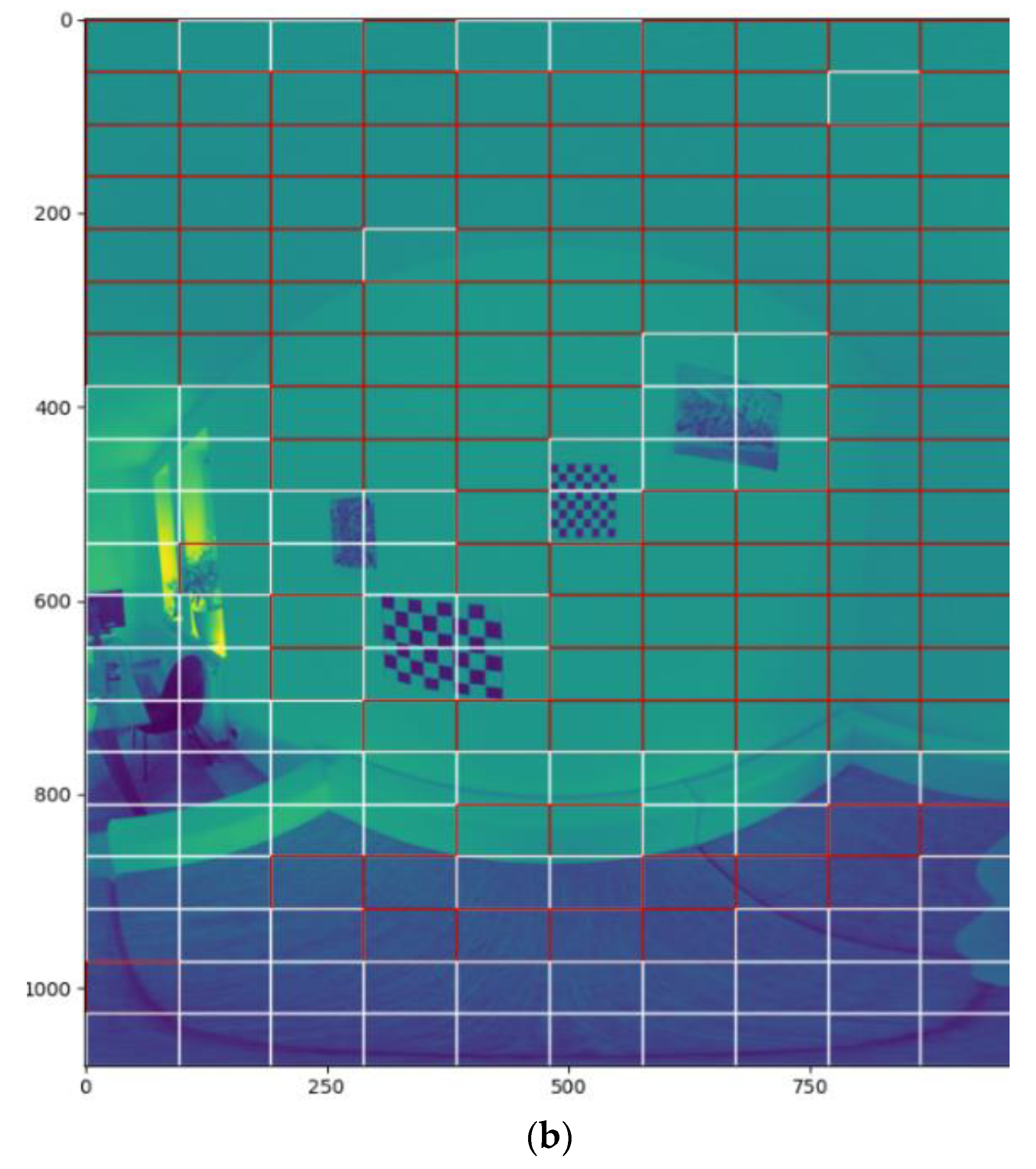
4.1. Frame Quality Calibration
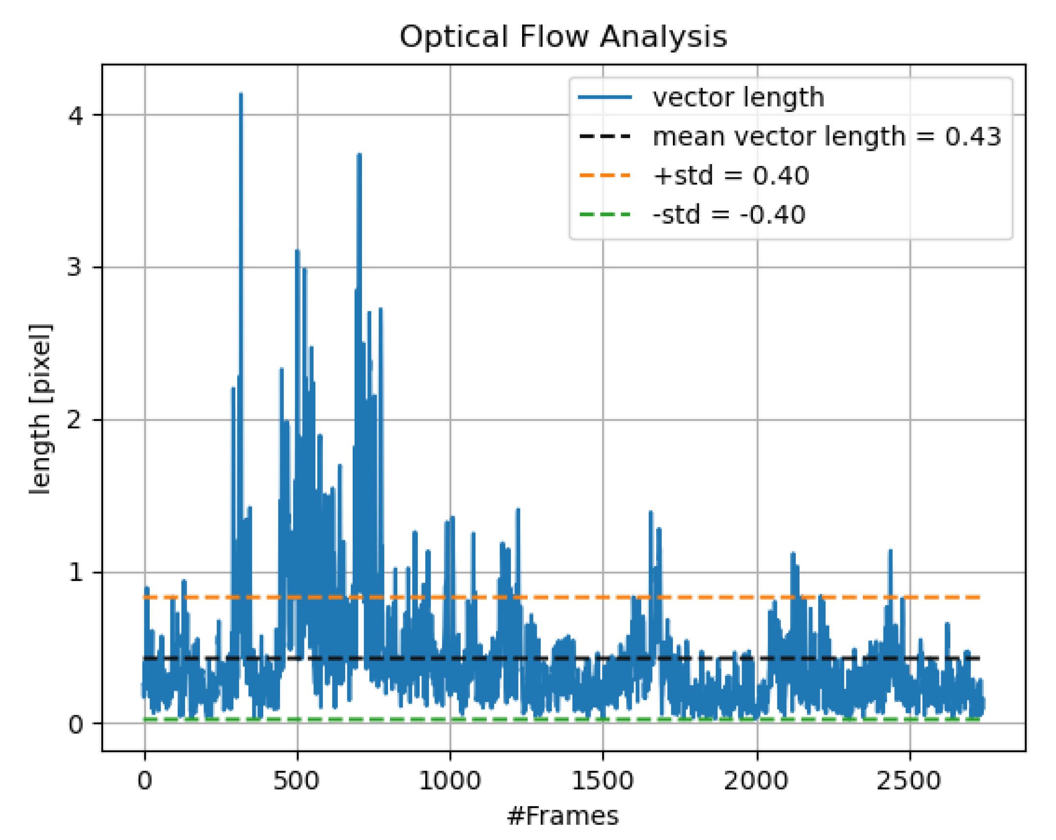
4.2. Frame Motion Calibraiton
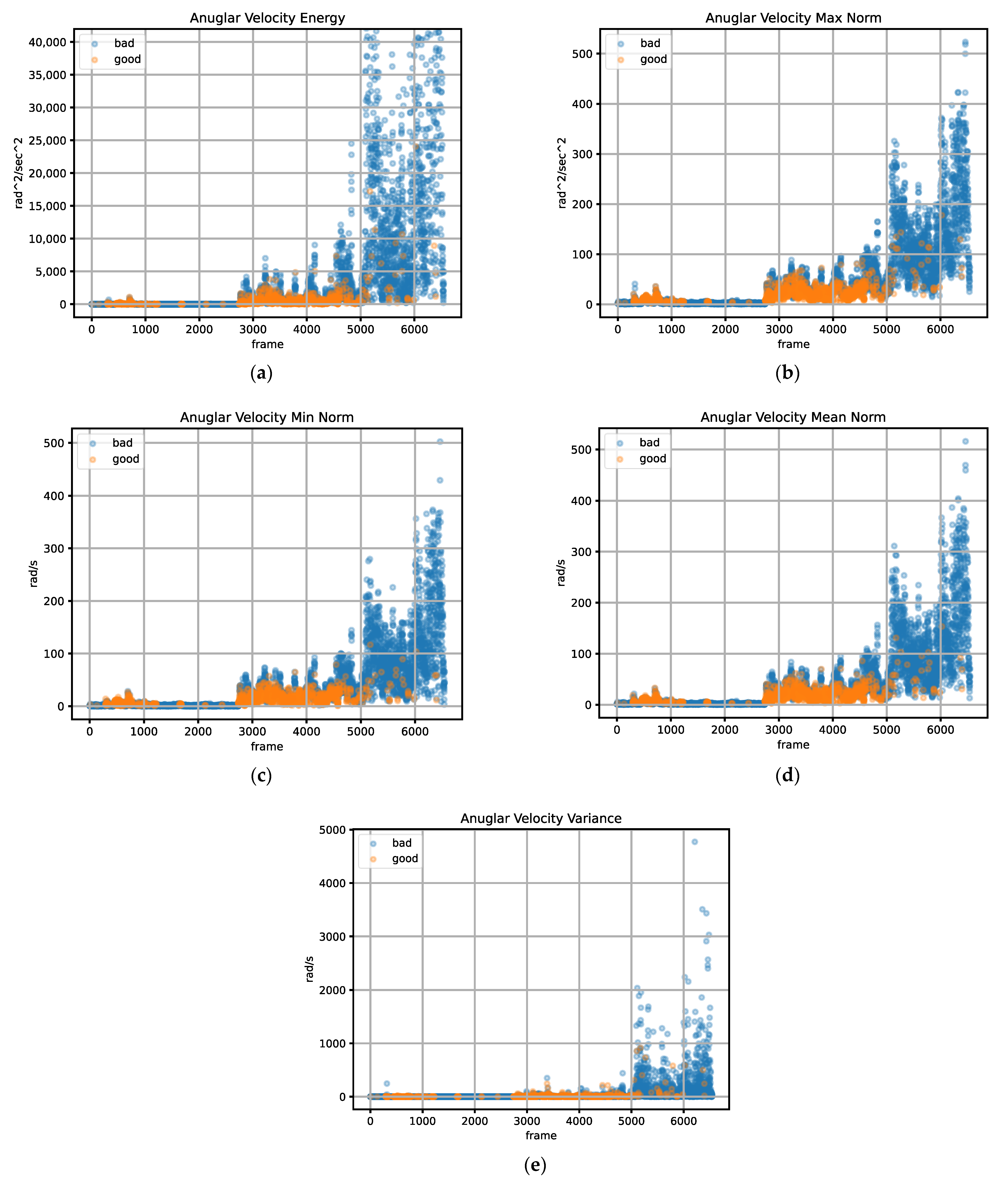
4.3. Feature Acquisition and Labeling
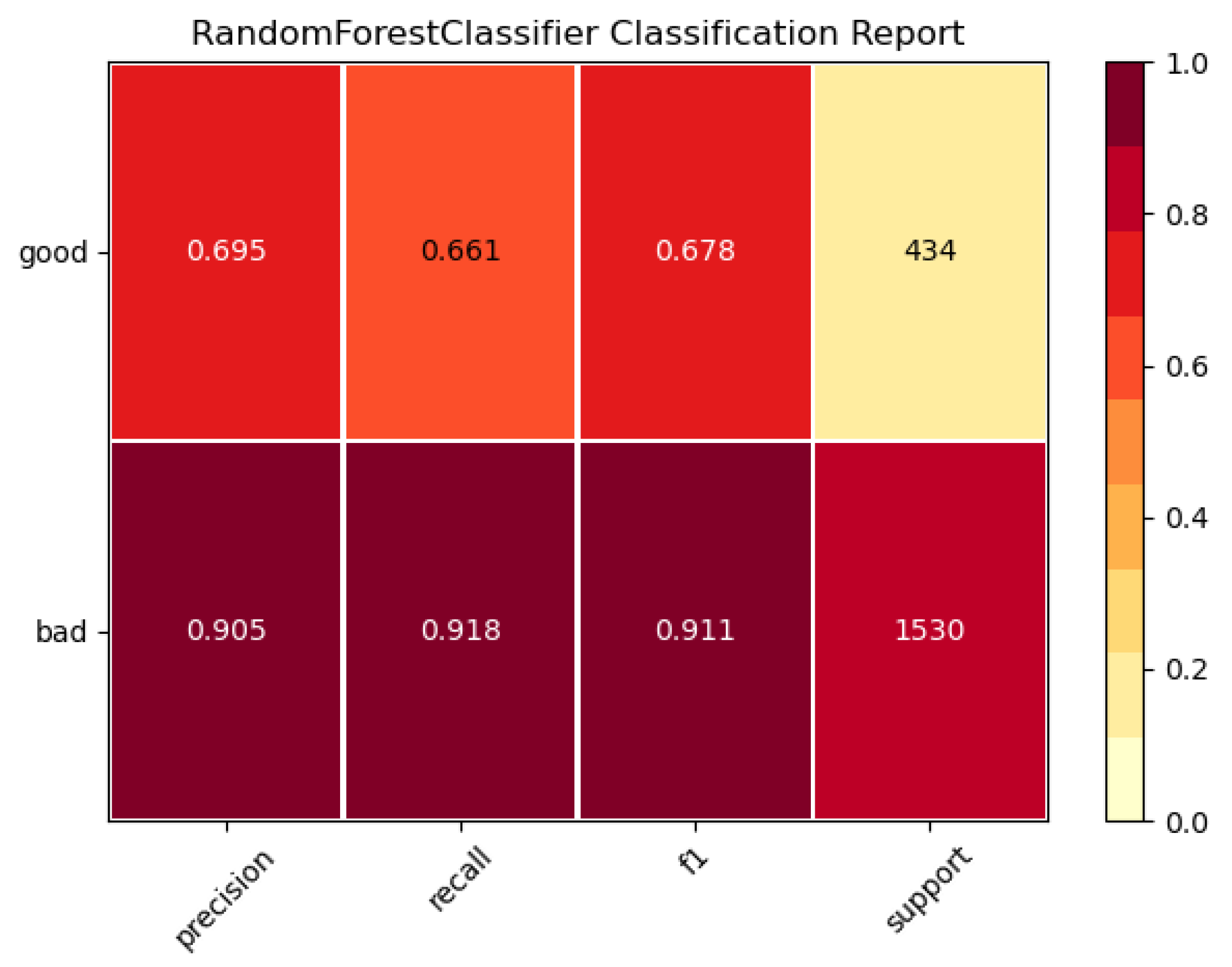
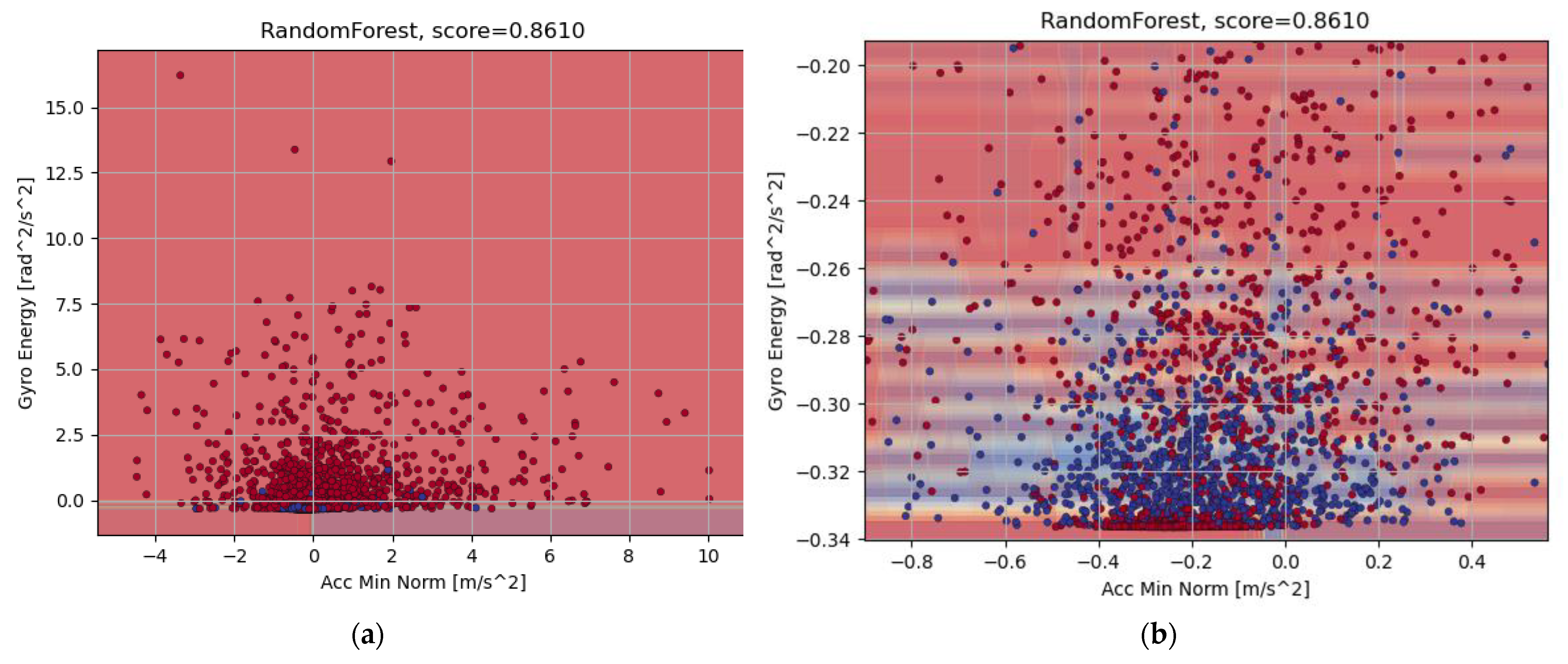
4.4. Classification
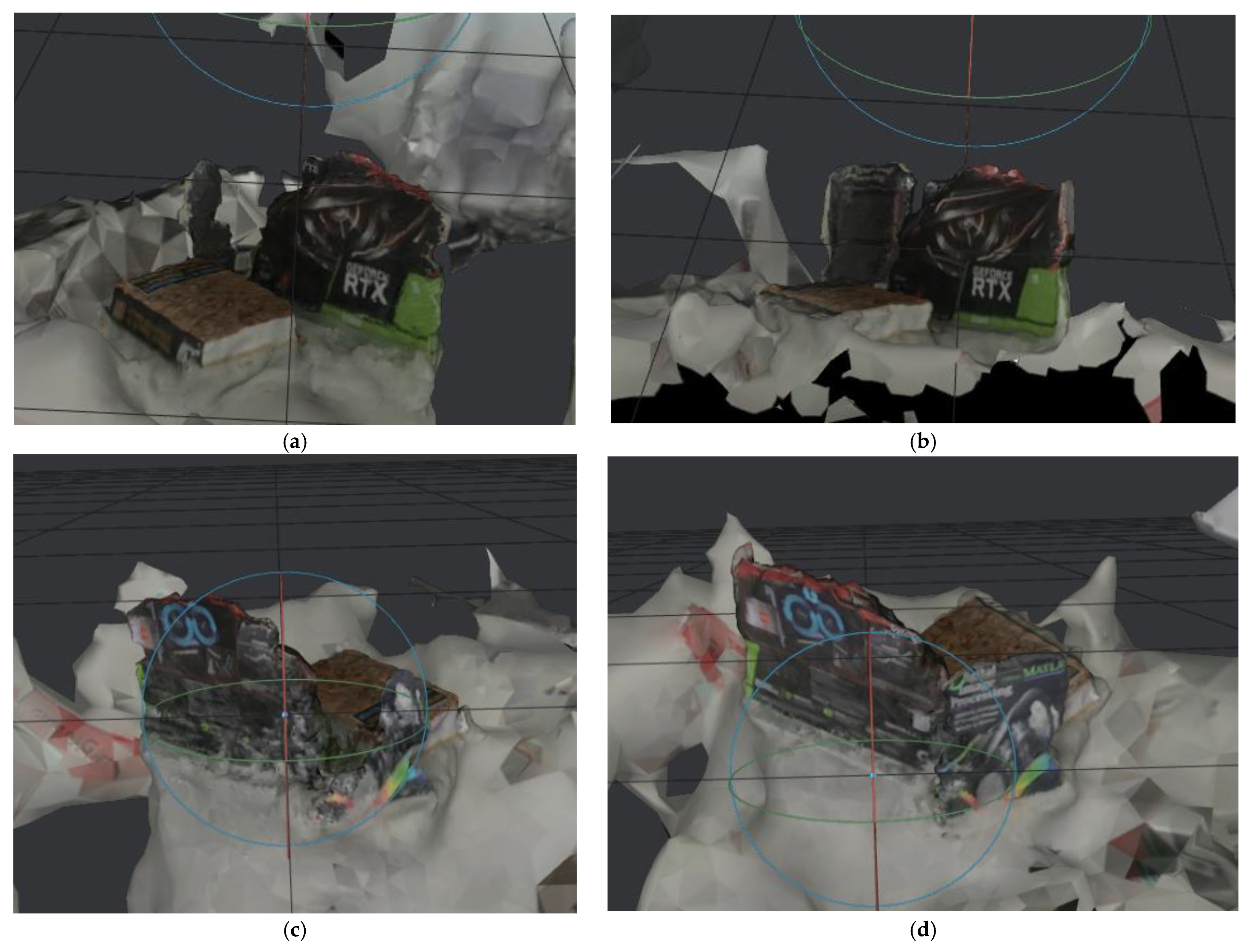
4.5. Reconstruction
5. Conclusions
Author Contributions
Funding
Institutional Review Board Statement
Informed Consent Statement
Data Availability Statement
Conflicts of Interest
References
- Reiterer, A.; Wäschle, K.; Störk, D.; Leydecker, A.; Gitzen, N. Fully Automated Segmentation of 2D and 3D Mobile Mapping Data for Reliable Modeling of Surface Structures Using Deep Learning. Remote Sens. 2020, 12, 2530. [Google Scholar] [CrossRef]
- Paar, G.; Huber, N.B.; Bauer, A.; Avian, M.; Reiterer, A. Vision-Based Terrestrial Surface Monitoring. Terrigenous Mass Mov. 2012, 283–348. [Google Scholar] [CrossRef]
- Péntek, Q.; Hein, S.; Miernik, A.; Reiterer, A. Image-based 3D surface approximation of the bladder using structure-from-motion for enhanced cystoscopy based on phantom data. Biomed. Technol. 2017, 63, 461–466. [Google Scholar] [CrossRef] [PubMed]
- Seibold, C.; Hilsmann, A.; Eisert, P. Model-based motion blur estimation for the improvement of motion tracking. Comput. Vis. Image Underst. 2017, 160, 45–56. [Google Scholar] [CrossRef]
- Ahmed, M.T.; Dailey, M.; Landabaso, J.; Herrero, N. Robust key frame extraction for 3D reconstruction from video strams. In Proceedings of the Fifth International Conference on Computer Vision Theory and Applications, Angers, France, 17–21 May 2010; pp. 231–236. [Google Scholar]
- Zhang, C.; Wang, H.; Li, H.; Liu, J. A fast key frame extraction algorithm and an accurate feature matching method for 3D reconstruction from aerial video. In Proceedings of the 29th Chinese Control and Decision Conference (CCDC), Chongqing, China, 28–30 May 2017; pp. 6744–6749. [Google Scholar]
- Ishijima, A.; Schwarz, R.A.; Shin, D.; Mondrik, S.; Vigneswaran, N.; Gillenwater, A.M.; Anandasabapathy, S.; Richards-Kortum, R. Automated frame selection process for high-resolution microendoscopy. J. Biomed. Opt. 2015, 20, 46014. [Google Scholar] [CrossRef] [PubMed] [Green Version]
- Ren, J.; Shen, X.; Lin, Z.; Mech, R. Best frame selection in a short video. In Proceedings of the 2020 IEEE Winter Conference on Applications of Computer Vision (WACV), Snowmass Village, CO, USA, 1–5 March 2020; IEEE: Piscataway, NJ, USA, 2020; pp. 3201–3210. [Google Scholar]
- Lucas, B.D.; Kanade, T. An iterative image registration technique with an application to stereo vision. Proceedings DARPA Image Understanding Workshop, Columnia, UK, 24–28 August 1981; pp. 121–130. [Google Scholar] [CrossRef]
- Yuen, M.; Wu, H. A survey of hybrid MC/DPCM/DCT video coding distortions. Signal Process. 1998, 70, 247–278. [Google Scholar] [CrossRef]
- Gonzales, R.C.; Woods, R.E. Digital Image Processing; Pearson/Prentice Hall: Upper Saddle River, NJ, USA, 2008; Available online: http://sdeuoc.ac.in/sites/default/files/sde_videos/Digital%20Image%20Processing%203rd%20ed.%20-%20R.%20Gonzalez%2C%20R.%20Woods-ilovepdf-compressed.pdf (accessed on 28 January 2021).
- Jähne, B. Digitale Bildverarbeitung; Springer: Berlin/Heidelberg, Germany, 2005; pp. 29–79. [Google Scholar] [CrossRef]
- Rekleitis, J. Visual Motion Estimation Based on Motion Blur Interpretation. School of Computer Science, McGill University. 1996. Available online: https://www.researchgate.net/publication/2687203_Visual_Motion_Estimation_based_on_Motion_Blur_Interpretation (accessed on 23 February 2021).
- Kalalembang, E.; Usman, K.; Gunawan, I.P. DCT-based local motion blur detection. In Proceedings of the International Conference on Instrumentation, Communication, Information Technology, and Biomedical Engineering, Bandung, Indonesia, 23–25 November 2009; pp. 1–6. [Google Scholar]
- Barron, J.L.; Fleet, D.J.; Beauchemin, S.S. Performance of optical flow techniques. Int. J. Comput. Vis. 1994, 12, 43–77. [Google Scholar] [CrossRef]
- Lowe, D.G. Distinctive Image Features from Scale-Invariant Keypoints. Int. J. Comput. Vis. 2004, 60, 91–110. [Google Scholar] [CrossRef]
- Harris, C.; Stephens, M. A Combined Corner and Edge Detector. Alvey Vis. Conf. 1988, 15, 10–5244. [Google Scholar] [CrossRef]
- OpenCV. Open Source Computer Vision Library; Intel: Clara, CA, USA, 2015. [Google Scholar]
- Shi, J.; Tomasi, C. Good Features to Track. In Proceedings of the IEEE Conference on Computer Vision and Pattern Recognition, Seattle, DC, USA, 21–23 June 1994; pp. 593–600. [Google Scholar]
- Kasebzadeh, P.; Hendeby, G.; Fritsche, C.; Gunnarsson, F.; Gustafsson, F. IMU dataset for motion and device mode classification. In Proceedings of the 2017 International Conference on Indoor Positioning and Indoor Navigation (IPIN), Sapporo, Japan, 18–21 September 2017; IEEE: Piscataway, NJ, USA, 2017; pp. 1–8. [Google Scholar]
- Susi, M.; Renaudin, V.; Lachapelle, G. Motion Mode Recognition and Step Detection Algorithms for Mobile Phone Users. Sensors 2013, 13, 1539–1562. [Google Scholar] [CrossRef] [PubMed]
- Pedregosa, F.; Varoquaux, G.; Gramfort, A.; Michel, V.; Thirion, B.; Grisel, O.; Blondel, M.; Prettenhofer, P.; Weiss, R.; Dubourg, V.; et al. Scikit-learn: Machine Learning in Python. J. Macm. Learn. Res. 2011, 12, 2825–2830. [Google Scholar]
- Alice, V. Meshroom: A 3D Reconstruction Software. 2018. Available online: https://github.com/alicevision/meshroom (accessed on 23 February 2021).


| Feature | Importance |
|---|---|
| 0.0434 | |
| (a) | 0.0457 |
| (a) | 0.0461 |
| (a) | 0.0429 |
| σ2(a) | 0.0533 |
| 0.1731 | |
| 0.2097 | |
| 0.1515 | |
| 0.1846 | |
| ) | 0.0493 |
| Params | Values w.r.t. Whole Set of Frames | Values w.r.t. Selected Key Frames by the Proposed Method |
|---|---|---|
| RMSE | 1.041 | 0.979758 |
| Processing time | 1163.54 s | 169.835 s |
| Number of frames | 1535 | 474 |
Publisher’s Note: MDPI stays neutral with regard to jurisdictional claims in published maps and institutional affiliations. |
© 2021 by the authors. Licensee MDPI, Basel, Switzerland. This article is an open access article distributed under the terms and conditions of the Creative Commons Attribution (CC BY) license (https://creativecommons.org/licenses/by/4.0/).
Share and Cite
Koschel, A.; Müller, C.; Reiterer, A. Selection of Key Frames for 3D Reconstruction in Real Time. Algorithms 2021, 14, 303. https://doi.org/10.3390/a14110303
Koschel A, Müller C, Reiterer A. Selection of Key Frames for 3D Reconstruction in Real Time. Algorithms. 2021; 14(11):303. https://doi.org/10.3390/a14110303
Chicago/Turabian StyleKoschel, Alan, Christoph Müller, and Alexander Reiterer. 2021. "Selection of Key Frames for 3D Reconstruction in Real Time" Algorithms 14, no. 11: 303. https://doi.org/10.3390/a14110303
APA StyleKoschel, A., Müller, C., & Reiterer, A. (2021). Selection of Key Frames for 3D Reconstruction in Real Time. Algorithms, 14(11), 303. https://doi.org/10.3390/a14110303