Author Contributions
Conceptualization, J.C., O.R.-S., D.A.A. and C.R.-C.; investigation, J.C., O.R.-S., D.A.A. and C.R.-C.; methodology, J.C., O.R.-S., D.A.A. and C.R.-C.; software, J.C. and C.R.-C.; resources J.C., O.R.-S. and C.R.-C.; supervision, J.C. and O.R.-S.; visualization, J.C., C.R.-C. and O.R.-S.; writing—original draft, J.C., C.R.-C., O.R.-S. and D.A.A.; writing—review and editing, J.C., C.R.-C. and O.R.-S. All authors have read and agreed to the published version of the manuscript.
Figure 1.
Overall primitive extraction process.
Figure 1.
Overall primitive extraction process.
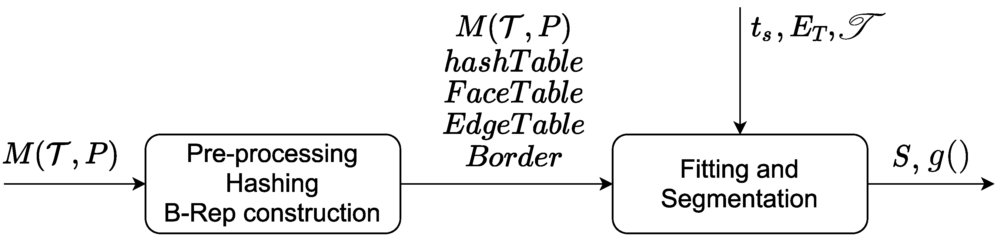
Figure 2.
Fitting process. Left (red) block: segmentation/fitting decoupled. Real-time identification of . Right (blue) block: codependent segmentation and fitting.
Figure 2.
Fitting process. Left (red) block: segmentation/fitting decoupled. Real-time identification of . Right (blue) block: codependent segmentation and fitting.
Figure 3.
(a) Bounding box and (b) rectangular voxel subdivision.
Figure 3.
(a) Bounding box and (b) rectangular voxel subdivision.
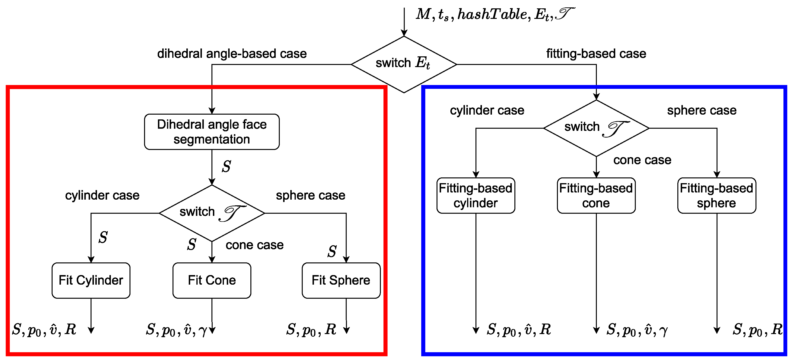
Figure 4.
Spatial hashing preprocessing. The hashing is executed before the fitting process starts.
Figure 4.
Spatial hashing preprocessing. The hashing is executed before the fitting process starts.
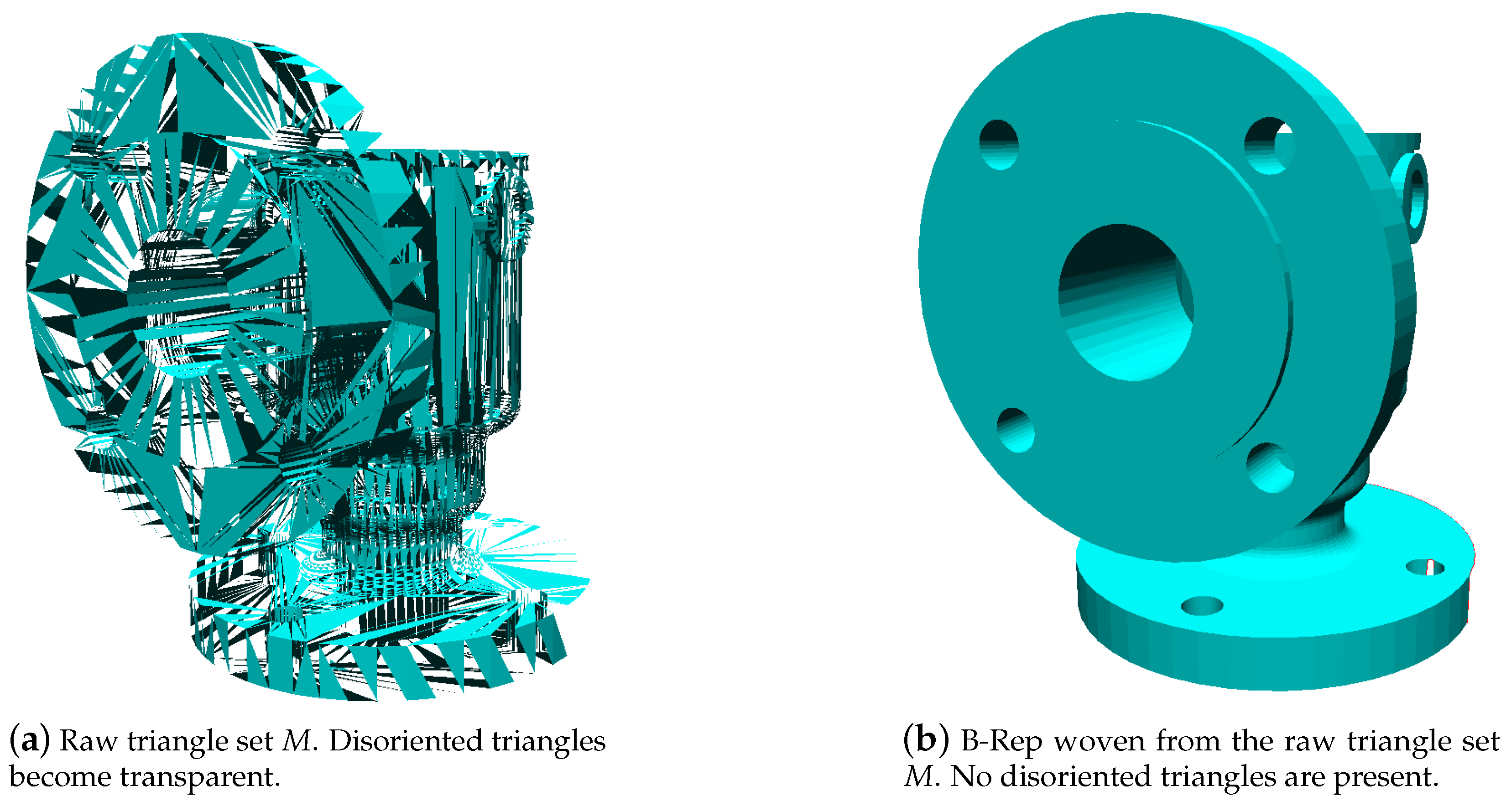
Figure 5.
Input triangle set M with inconsistent FACE orientation. Output B-Rep of M. (a) and (b) displayed with culling based on the triangle orientations.
Figure 5.
Input triangle set M with inconsistent FACE orientation. Output B-Rep of M. (a) and (b) displayed with culling based on the triangle orientations.
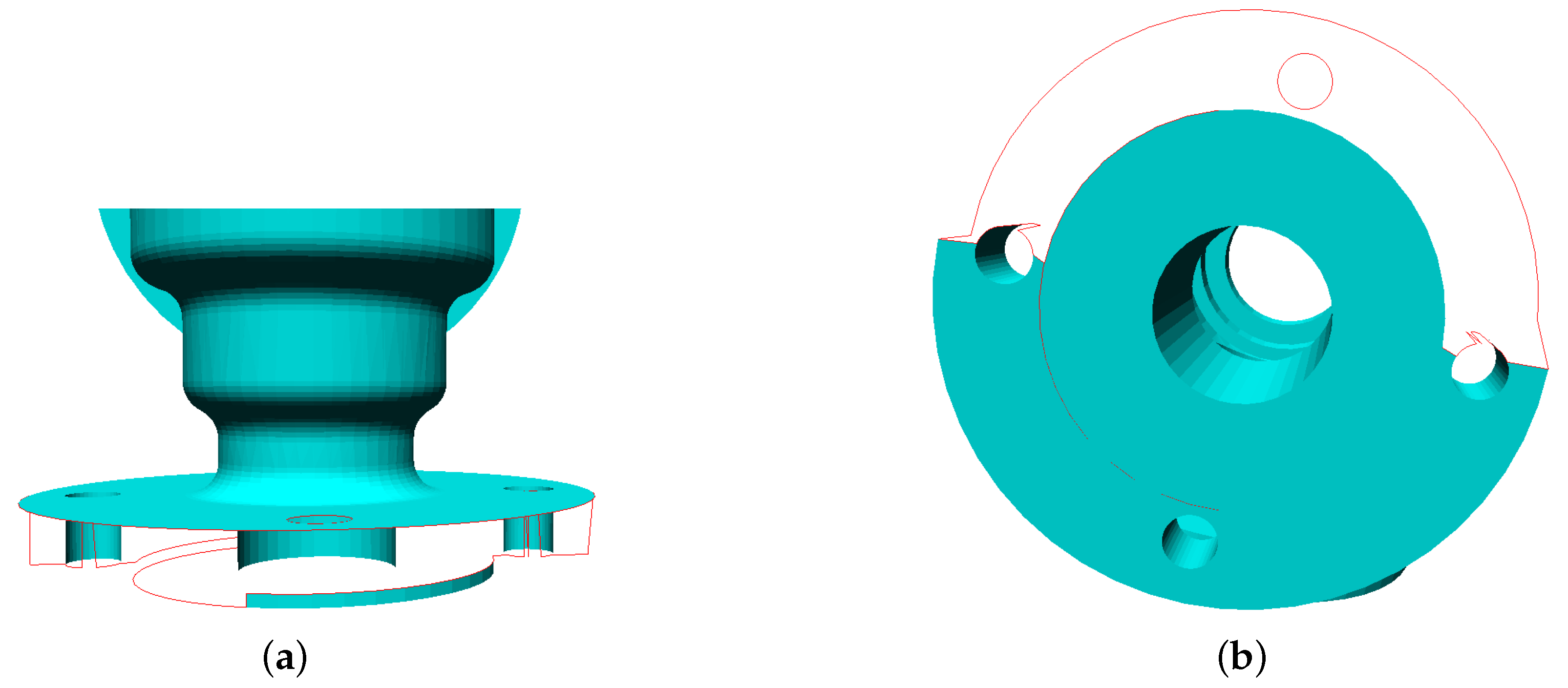
Figure 6.
Result of border identification in the triangle set. (a) and (b) present the identified border of the triangle set after weaving the B-Rep.
Figure 6.
Result of border identification in the triangle set. (a) and (b) present the identified border of the triangle set after weaving the B-Rep.
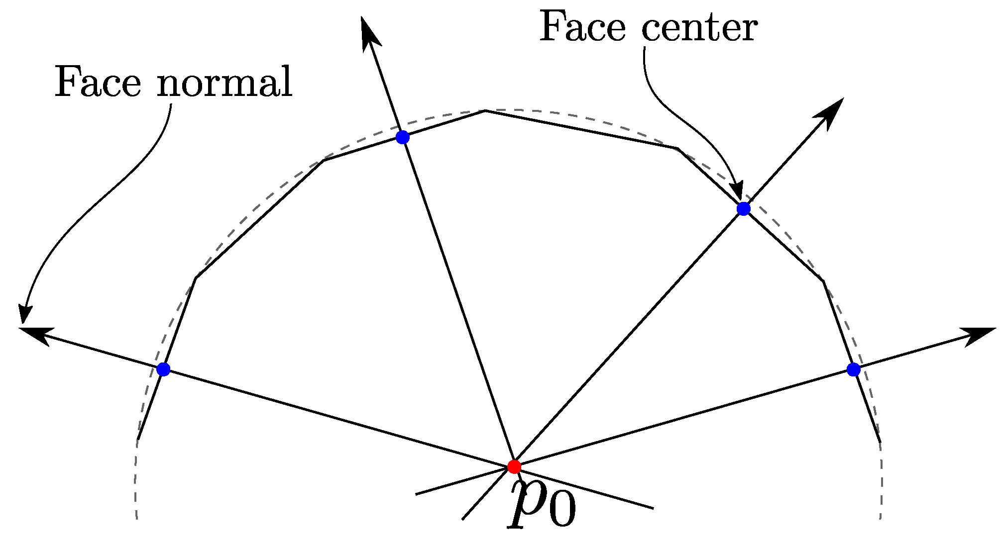
Figure 7.
calculation with the intersection of lines whose directions are triangle normal vectors and pass through triangle baricenters .
Figure 7.
calculation with the intersection of lines whose directions are triangle normal vectors and pass through triangle baricenters .
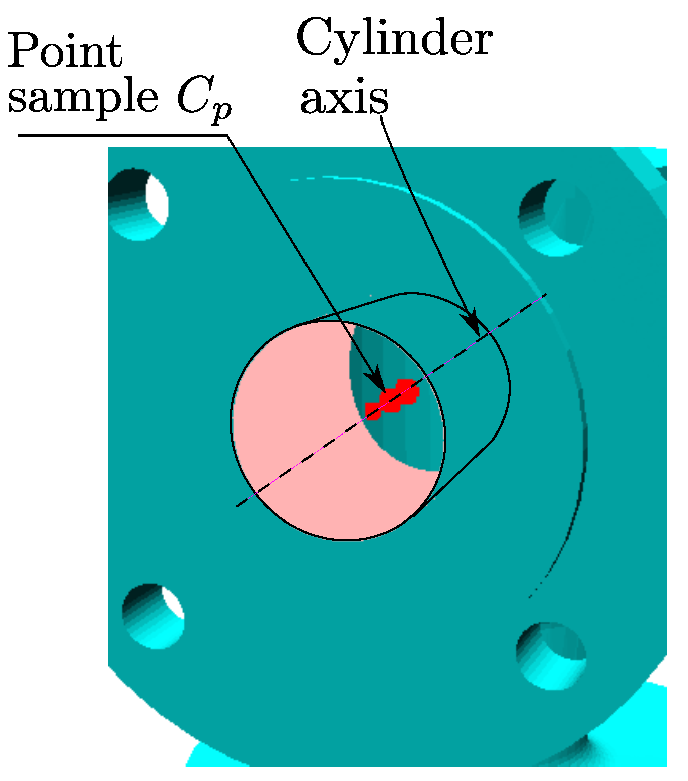
Figure 8.
Set of points approximating the cylinder axis.
Figure 8.
Set of points approximating the cylinder axis.
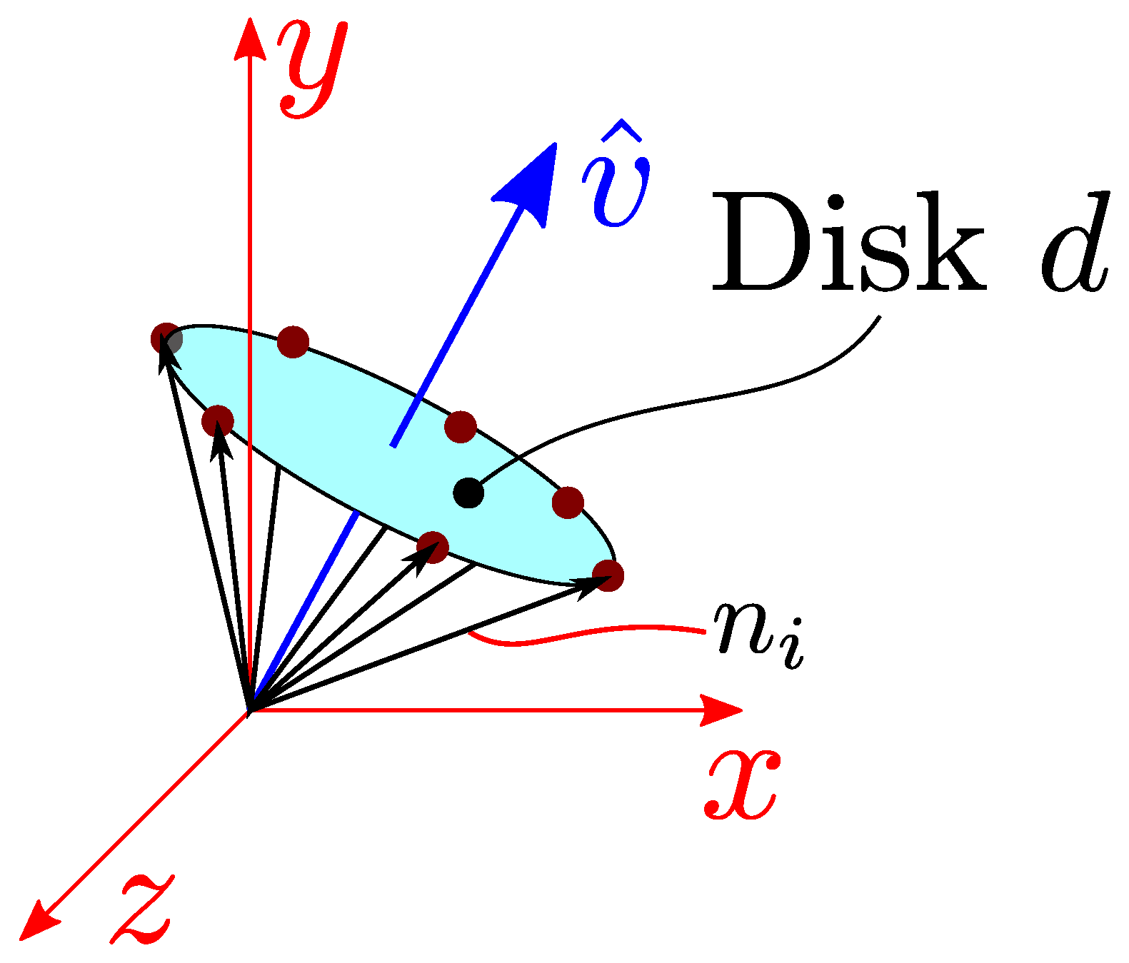
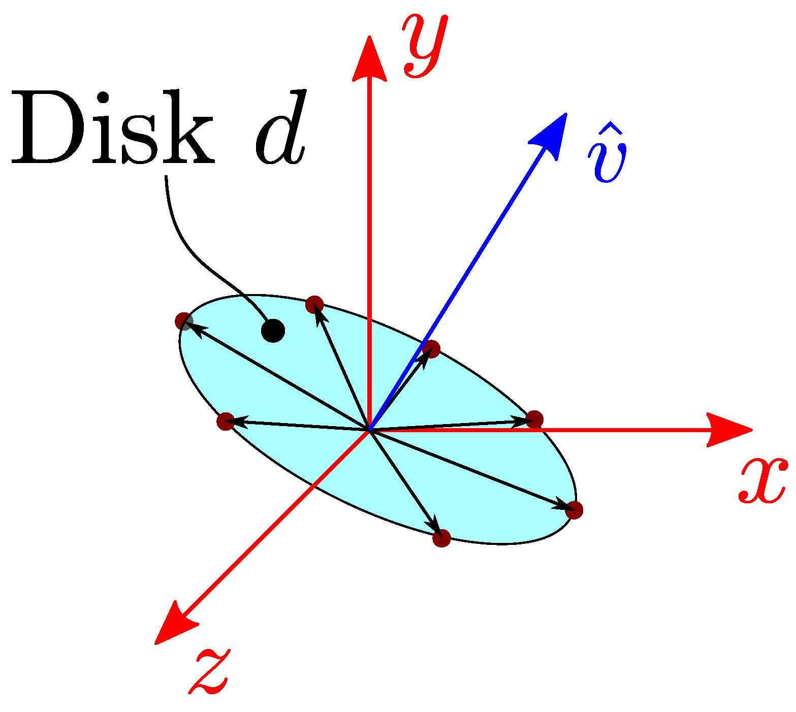
Figure 9.
Cylinder fitting. Coplanar circular set of tips of cylinder normal unitary vectors, applied at origin. : direction of minimal dispersion of disk d, cylinder axis direction.
Figure 9.
Cylinder fitting. Coplanar circular set of tips of cylinder normal unitary vectors, applied at origin. : direction of minimal dispersion of disk d, cylinder axis direction.
Figure 10.
Cone fitting. Dual cone formed with Origin as apex. Unitary vectors normal to S are generatrices for the dual cone. Origin-located tails of vectors normal to triangles at Origin. Normal vector tips contained in a plane form a flat disk d. Minimal dispersion direction (principal component analysis) of disk d is the direction of cone axis .
Figure 11.
Cone 2D example. Vectors point to and are perpendicular to .
Figure 11.
Cone 2D example. Vectors point to and are perpendicular to .
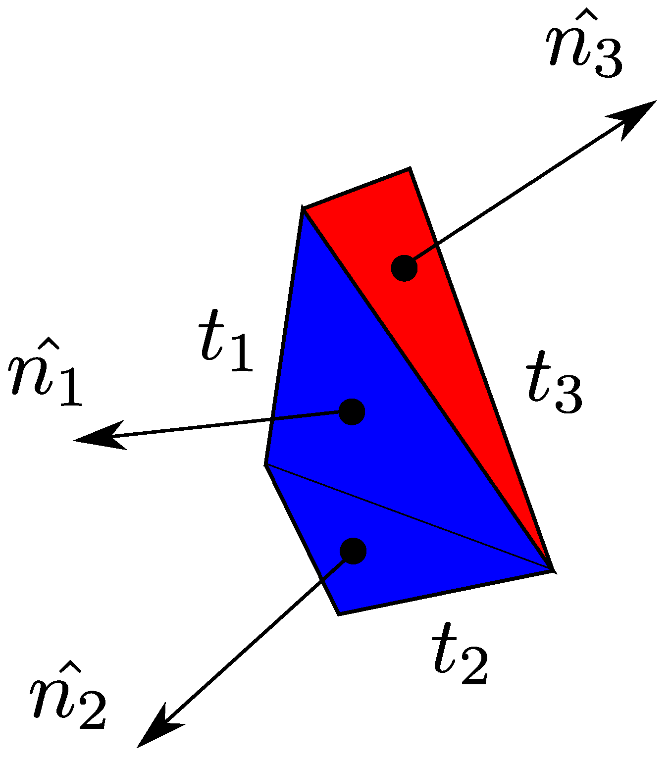
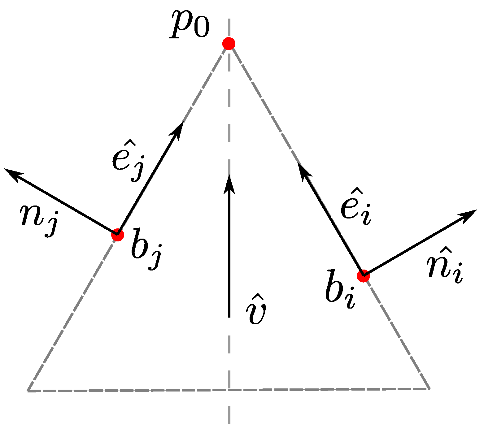
Figure 12.
Dihedral angle equivalence . and (blue equivalence class). and (red) is outside the equivalence class (blue) of and .
Figure 12.
Dihedral angle equivalence . and (blue equivalence class). and (red) is outside the equivalence class (blue) of and .
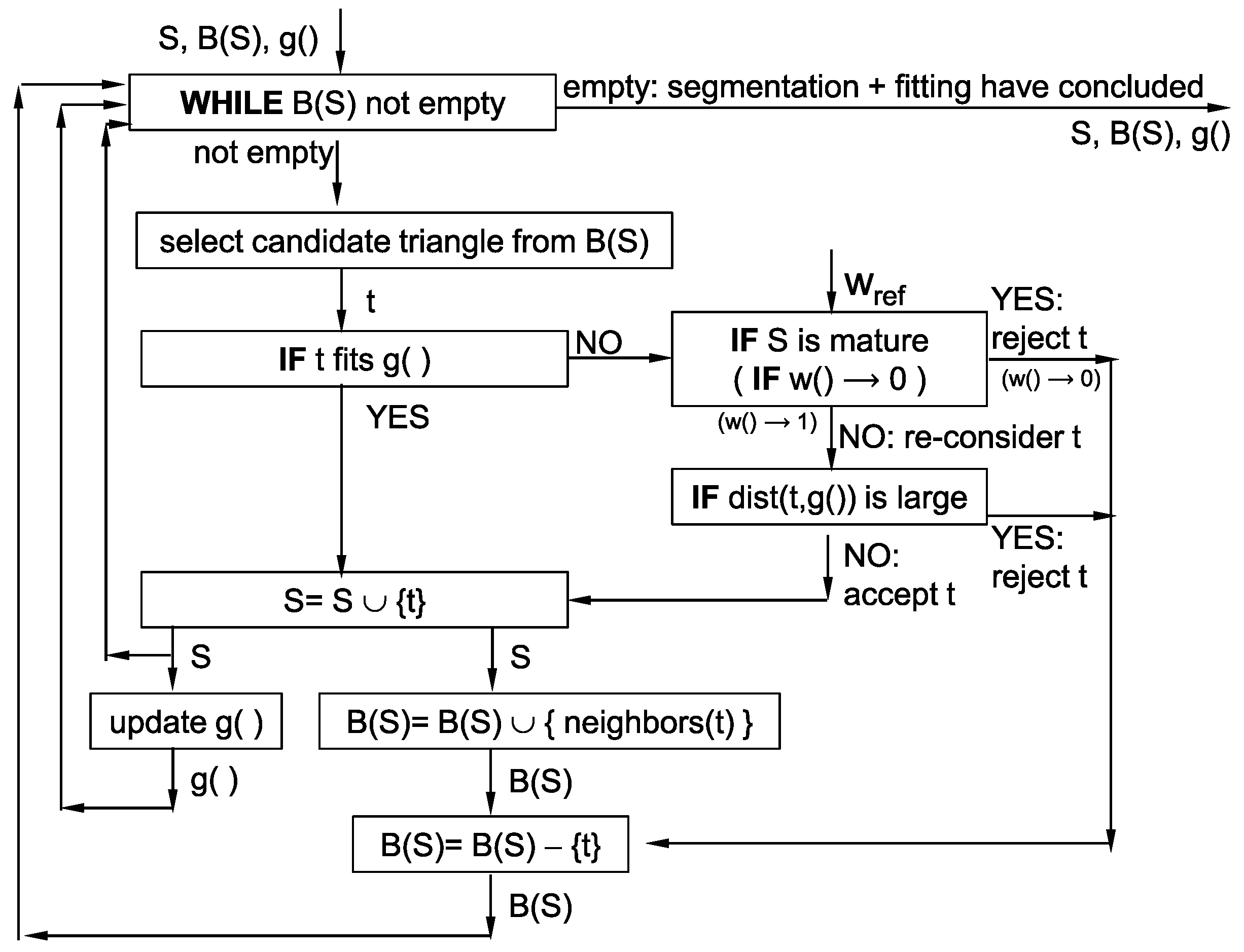
Figure 13.
Algorithm for simultaneous fitting of and extraction of support subset S.
Figure 13.
Algorithm for simultaneous fitting of and extraction of support subset S.
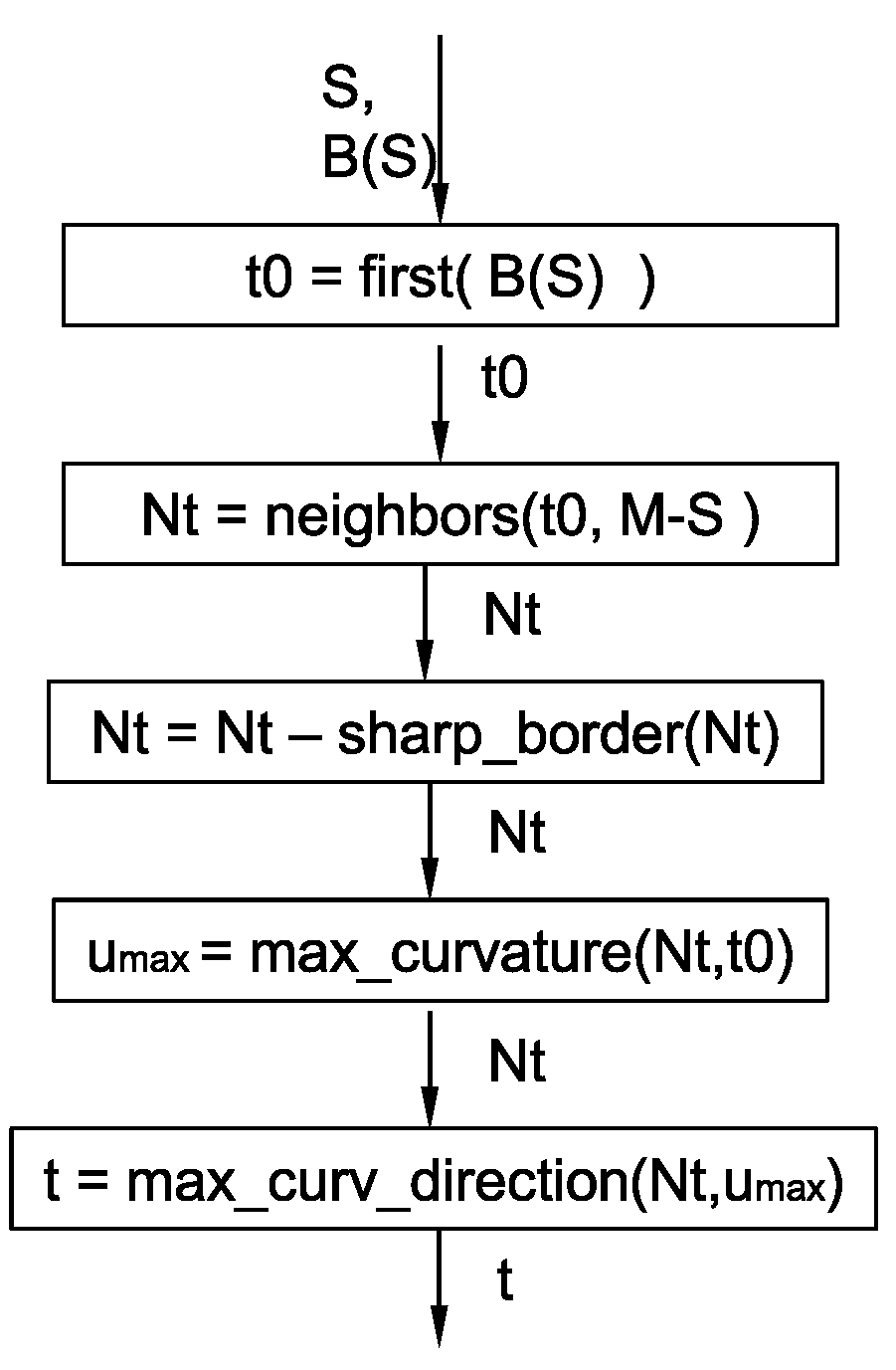
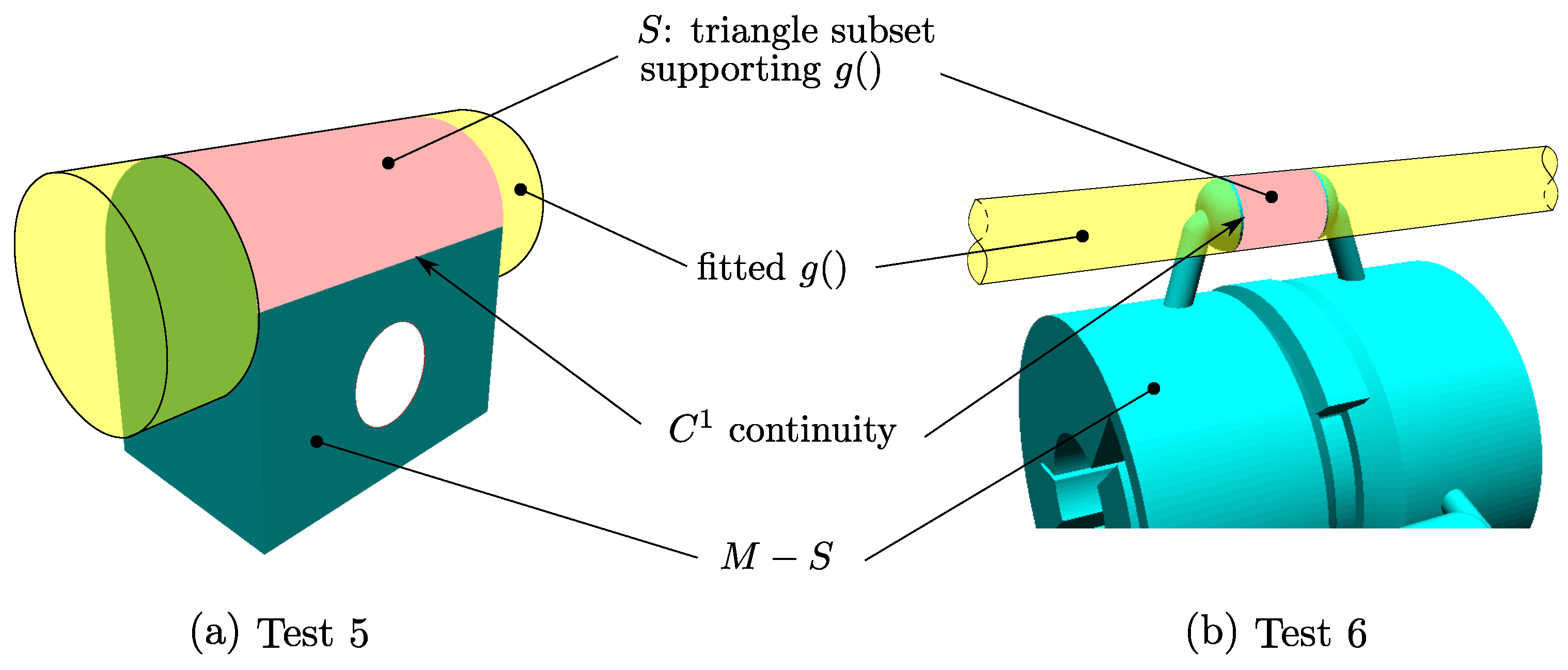
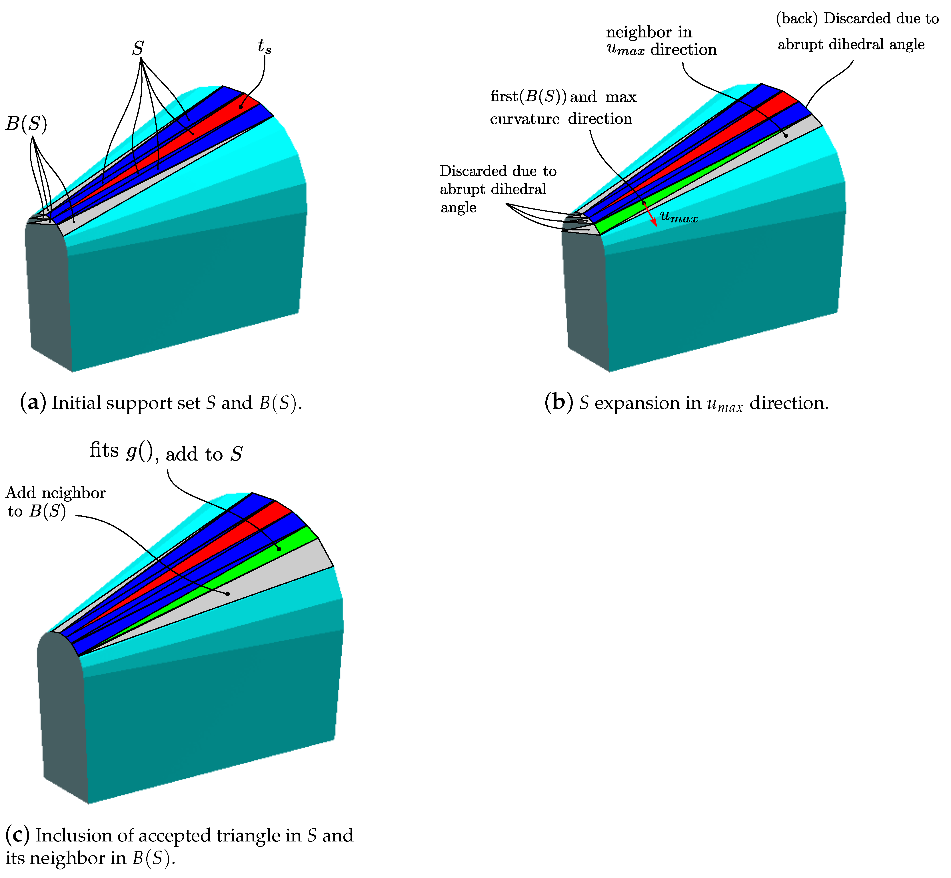
Figure 14.
Expansion of box/process “select candidate triangle from
” from
Figure 13.
Figure 14.
Expansion of box/process “select candidate triangle from
” from
Figure 13.
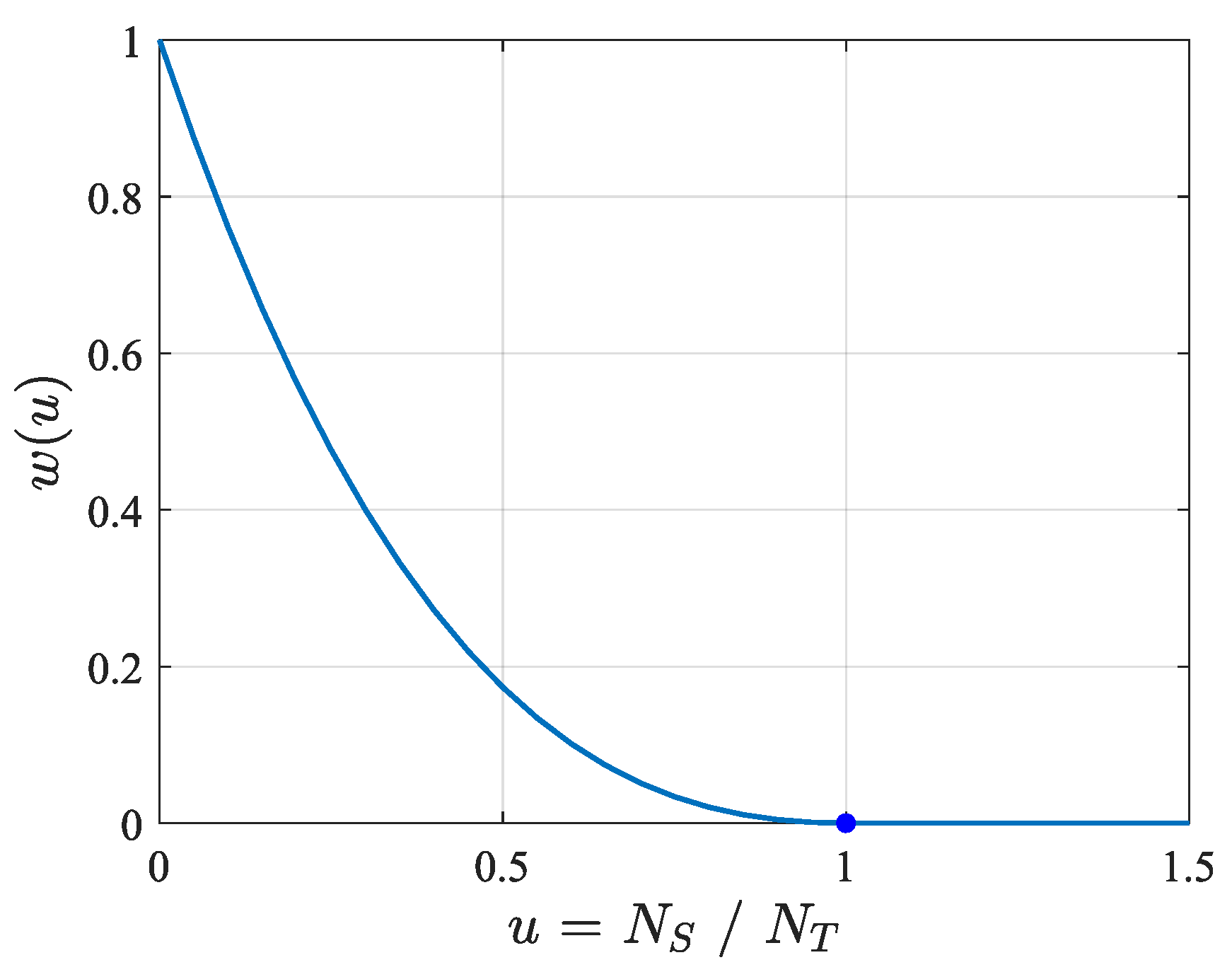
Figure 15.
S immaturity function . : S is immature set, with few triangles . : S is mature set, with many triangles ( ). threshold in number of triangles to consider as stable analytic form.
Figure 15.
S immaturity function . : S is immature set, with few triangles . : S is mature set, with many triangles ( ). threshold in number of triangles to consider as stable analytic form.
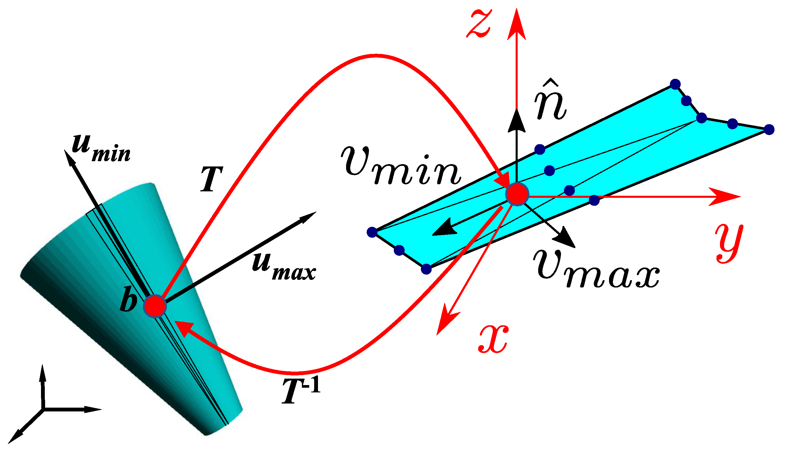
Figure 16.
Rigid mapping M of local tangent plane of a ruled surface S onto the plane for the purpose of computing maximal and minimal curvature directions on S.
Figure 16.
Rigid mapping M of local tangent plane of a ruled surface S onto the plane for the purpose of computing maximal and minimal curvature directions on S.
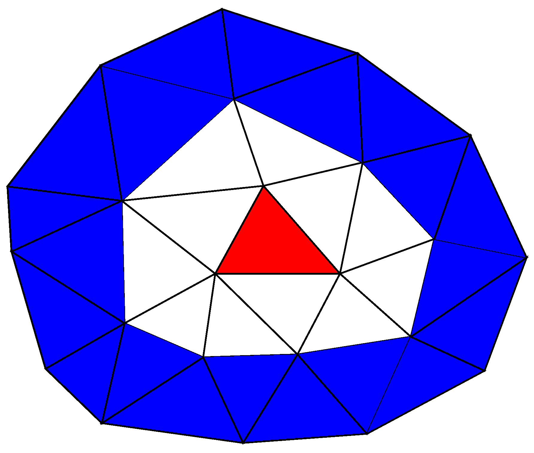
Figure 17.
Red: user input seed triangle (). Blue: topological circle . White: topological circle . Red + White + Blue: topological ball . The initial guess for the analytic form is computed with .
Figure 17.
Red: user input seed triangle (). Blue: topological circle . White: topological circle . Red + White + Blue: topological ball . The initial guess for the analytic form is computed with .
Figure 18.
Step-wise execution of the S extraction fitting algorithm, applied to a cone which does not accept S extraction based on dihedral angles.
Figure 18.
Step-wise execution of the S extraction fitting algorithm, applied to a cone which does not accept S extraction based on dihedral angles.
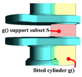
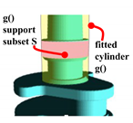
Figure 19.
Cylinder fit. S extraction based on dihedral angles. Pink: extracted S support subset. Yellow: fitted .
Figure 19.
Cylinder fit. S extraction based on dihedral angles. Pink: extracted S support subset. Yellow: fitted .
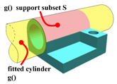
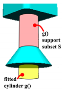
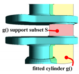
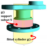
Figure 20.
Cylinder fit. Fitting-based S extraction. Pink: extracted S support subset. Yellow: fitted .
Figure 20.
Cylinder fit. Fitting-based S extraction. Pink: extracted S support subset. Yellow: fitted .
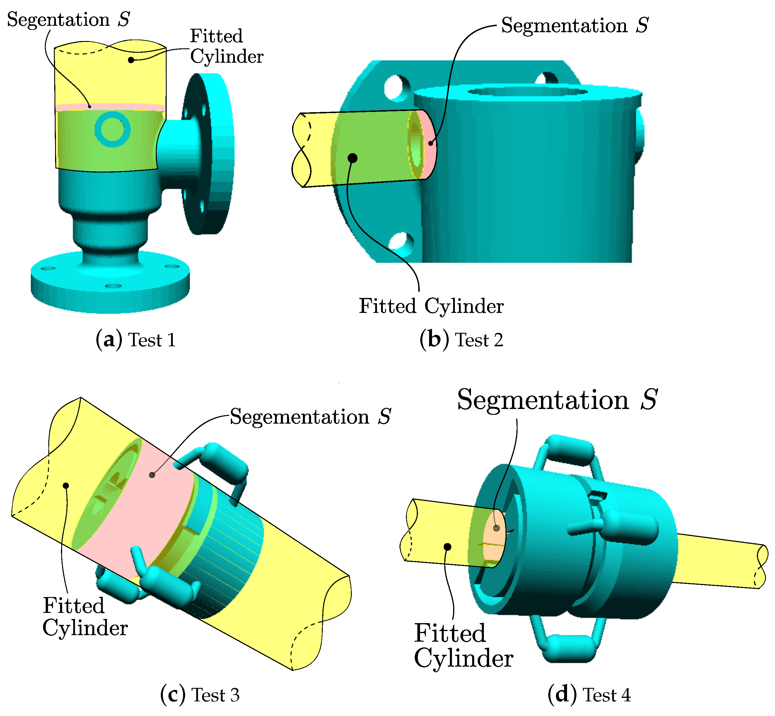
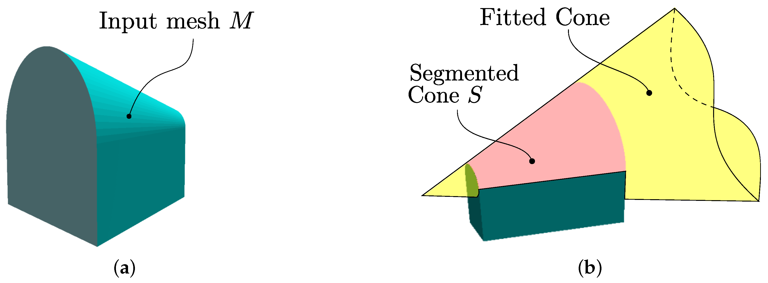
Figure 21.
Test 1. Cone fitting test using dihedral angle-based extraction. Pink: segmentation. Yellow: cone fitting.
Figure 21.
Test 1. Cone fitting test using dihedral angle-based extraction. Pink: segmentation. Yellow: cone fitting.
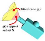
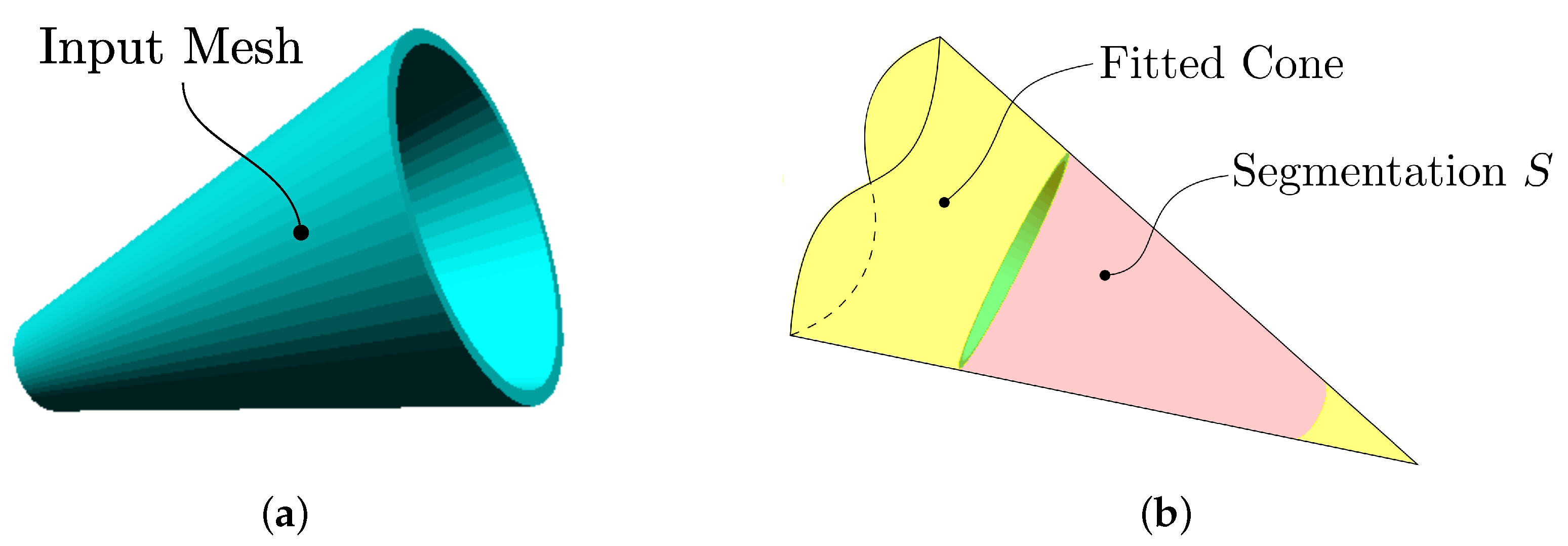
Figure 22.
Cone Fit. Fitting-based S extraction. Pink: extracted S support subset. Yellow: fitted .
Figure 22.
Cone Fit. Fitting-based S extraction. Pink: extracted S support subset. Yellow: fitted .
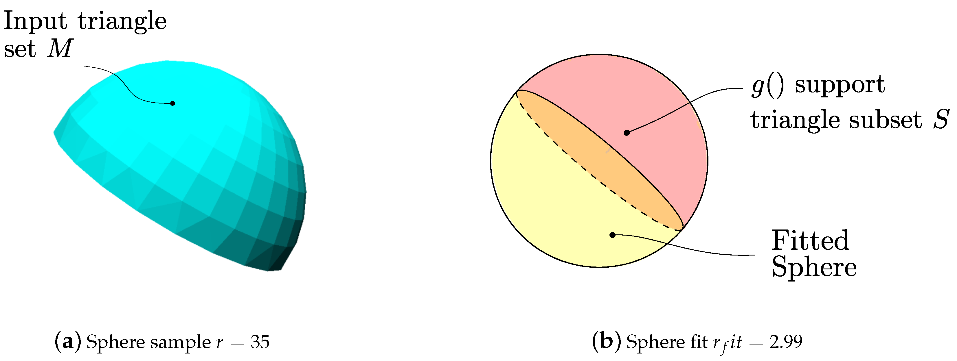
Figure 23.
Sphere fitting using dihedral angle-based extraction. Pink: segmented sphere. Yellow: fitted sphere. Notice that .
Figure 23.
Sphere fitting using dihedral angle-based extraction. Pink: segmented sphere. Yellow: fitted sphere. Notice that .
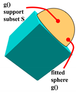
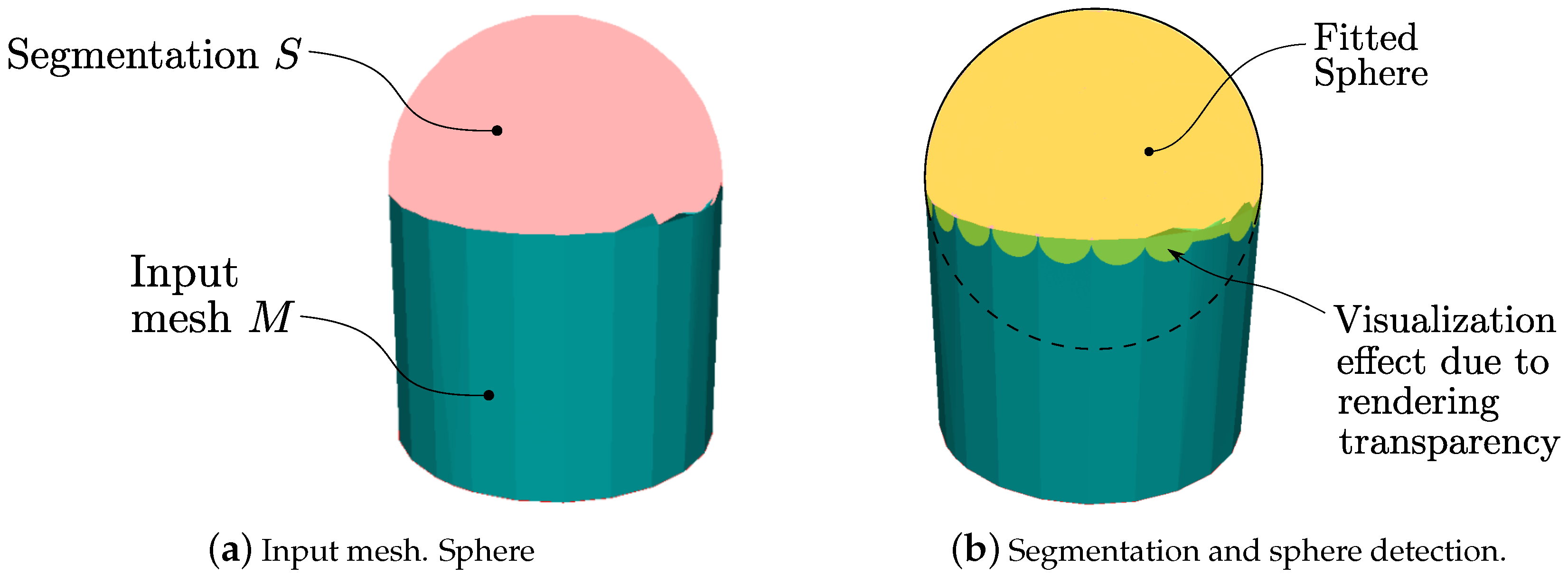
Figure 24.
Sphere fit. Fitting-based S extraction. Pink: extracted S support subset. Yellow: fitted . The process leaves out of S few sphere triangles at the border with . However, it succeeds in rejecting inclusion in S of triangles actually belonging to the cylinder.
Figure 24.
Sphere fit. Fitting-based S extraction. Pink: extracted S support subset. Yellow: fitted . The process leaves out of S few sphere triangles at the border with . However, it succeeds in rejecting inclusion in S of triangles actually belonging to the cylinder.
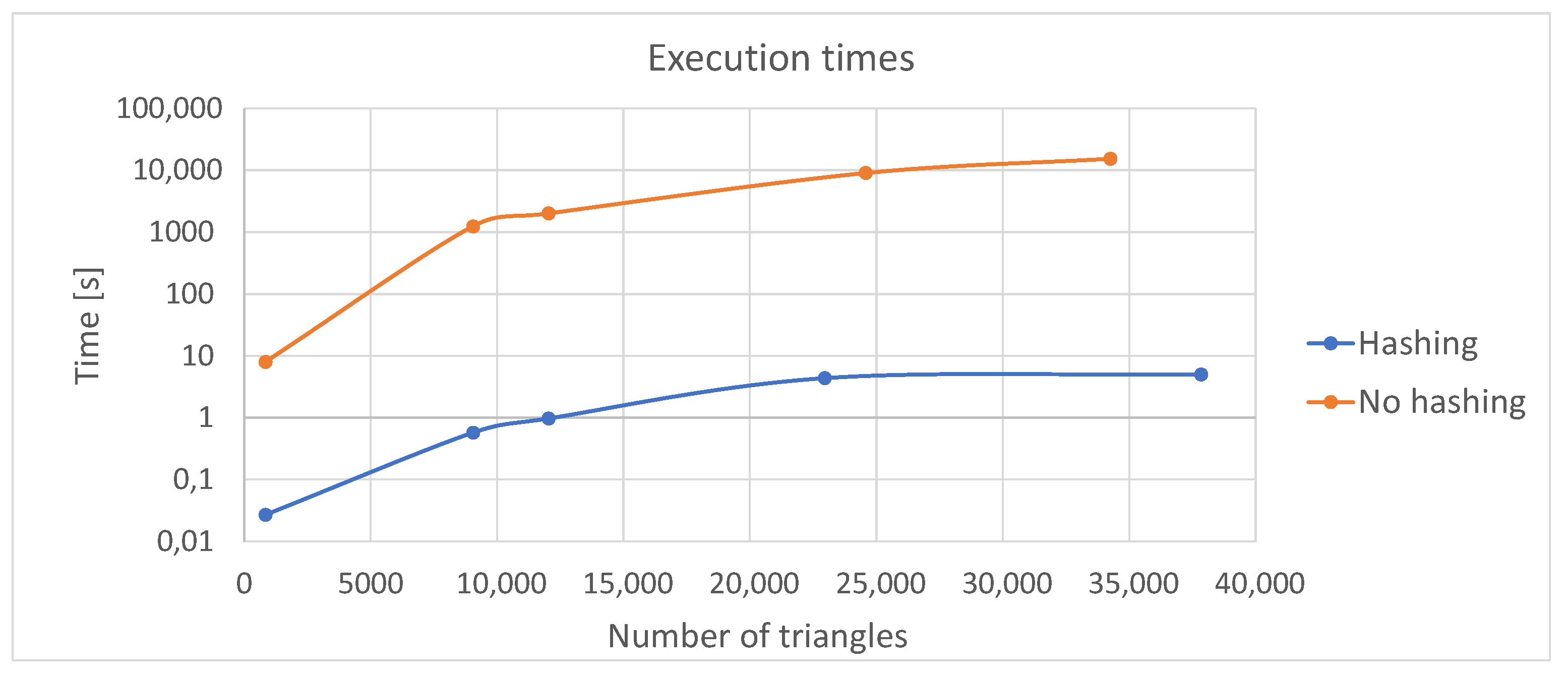
Figure 25.
Execution times for B-Rep construction with and without previous spatial hashing.
Figure 25.
Execution times for B-Rep construction with and without previous spatial hashing.
Table 1.
Competitor approaches vs. current approach.
Table 1.
Competitor approaches vs. current approach.
| Approach | Refs. | Advantages | Disadvantages |
|---|
| Stochastic Methods. Randomly apply local regressions of alternative goal primitives and keeping the best fit. | [2,3,10,11,12] | (1) Robust to outliers; (2) application-specific | (1) Requires dense, isotropic, homogeneous input dataset. |
| Mapping to Parameter Space. Implement a mapping to the parameter space, identify the number of parameters needed and search for clusters of similar parameters. | [4,5,13,14] | (1) Robust to noise and outliers; (2) work with missing data | (1) High computational cost; (2) requires dense datasets |
| Mesh Segmentation Fitting Methods. Create clusters of the dataset using different grouping techniques. Fitting can occur during or after the segmentation. | [6,7,8,9,15,16,17] | (1) Spatial consistency | (1) Sensitive to noise and outliers; (2) require supplementary information in the dataset. |
| Our approach. A primitive fitting in poor triangular meshes. Segmentation driven by dihedral angle is implemented when continuity is strict . Segmentation and fitting are codependent for or higher continuity. | | (1) Fitting in poor datasets; (2) low computational cost; (3) real-time performance for -continuity; (4) perfecting of S for or higher continuity. | (1) Requires the type of analytic form intended to be fitted as an input. |
Table 2.
VERTEX table.
| Vertex | x | y | z | Edge |
|---|
| 1 | 2.34 | 3.00 | 1.12 | 13 |
| 2 | 2.22 | 9.00 | 10.36 | 27 |
| 3 | 5.20 | 4.00 | 9.12 | 53 |
Table 3.
FACE table constructed from B-Rep.
Table 3.
FACE table constructed from B-Rep.
| Face | Edge 1 | Edge 2 | Edge 3 |
|---|
| 1 | 1 | 2 | 3 |
| 2 | 3 | 5 | 4 |
| 3 | 3 | 1 | 4 |
Table 4.
EDGE table. If counter-EDGE cell is empty, indicates border.
Table 4.
EDGE table. If counter-EDGE cell is empty, indicates border.
| Edge | Vertex 1 | Vertex 2 | Counter-EDGE | Face |
|---|
| 1 | 1 | 2 | 4 | 1 |
| 2 | 2 | 3 | 5 | 1 |
| 3 | 3 | 4 | - | 1 |
Table 5.
BORDER table.
| Border Loop | Vertex 1 | Vertex 2 | Vertex 3 | Vertex 4 | Vertex 5 | Vertex 6 | … |
|---|
| 1 | 4 | 7 | 8 | 91 | <End-of-loop> | | |
| 2 | 10 | 71 | 31 | 11 | 1 | 90 | <End-of-loop> |
| 3 | 63 | 83 | 47 | 121 | 9 | <End-of-loop> | |
Table 6.
Cylinder fit. Set vs. found parameters. Tests 1–4: S extraction based on dihedral angles. Tests 5–6: Fitting-based S extraction.
Table 6.
Cylinder fit. Set vs. found parameters. Tests 1–4: S extraction based on dihedral angles. Tests 5–6: Fitting-based S extraction.
| | R | | | | Degrees |
|---|
| Test #1 | 47 | 46.9999 | | | 0 |
| Test #2 | 14 | 13.9972 | | | 0.0497 |
| Test #3 | 13 | 13.00004 | | | 0.0136 |
| Test #4 | 5 | 5.0037 | | | 0.0051 |
| Test #5 | 20 | 20.0000 | | | 0 |
| Test #6 | 2.5 | 2.4999 | | | 0 |
Table 7.
Cone fit. Set vs. found parameters. Test 1: S extraction based on dihedral angles. Test 2: fitting-based S extraction.
Table 7.
Cone fit. Set vs. found parameters. Test 1: S extraction based on dihedral angles. Test 2: fitting-based S extraction.
| | | | | | | | Degrees |
|---|
| Test #1 | | | 13.87 | 13.8852 | | | 0.0033 |
| Test #2 | | | 19 | 18.9716 | | | 0.0033 |
Table 8.
SPHERE Fit. Set vs. found parameters. Test 1: S extraction based on dihedral angles. Test 2: fitting-based S extraction.
Table 8.
SPHERE Fit. Set vs. found parameters. Test 1: S extraction based on dihedral angles. Test 2: fitting-based S extraction.
| | R | | | |
|---|
| Test #1 | 3 | 2.9752 | | |
| Test #2 | 25 | 25.0216 | | |
Table 9.
Test with reference datasets of competitor approaches.
Table 10.
Complexities of existing approaches and of our algorithm (n is the number of points or triangles of the input set). Obtaining initial guess of . Applying optimization to . Segmentation and fitting are codependent.
Table 10.
Complexities of existing approaches and of our algorithm (n is the number of points or triangles of the input set). Obtaining initial guess of . Applying optimization to . Segmentation and fitting are codependent.
| Approach | Preprocessing | B-Rep | Extraction of S | Fitting | Extraction + Fitting † | Overall |
|---|
| [7] Yan et al. | | - | | | | |
| [6] Attene et al. | | - | - | - | | |
| [3] Ruiz et al. | | - | - | | - | |
| [12] Li et al. | | - | | | | |
| [4] Hulik et al. | | - | - | | - | |
| Our approach | | | | | | |


