1. Introduction
The majority of machine learning projects tend to follow the same pattern, namely, many different machine learning model types (such as decision trees, logistic regression, random forest, neural network, etc.) are first trained from data to predict specific outcomes, and then tested and compared to find the one that gives the best prediction performance on validation data. Many techniques to compare models have been developed and are commonly used in several settings [
1,
2,
3]. For some specific model types, such as neural networks, it is difficult to know when to stop the search [
4]. There is always the hope that a different set of hyperparameters, as the number of layers, or a better optimizer, will give a better performance [
4,
5]. This makes the model comparison laborious and time-consuming.
Many reasons may lead to a bad accuracy: deficiencies in the classifier, overlapping class densities [
6,
7], noise affecting the data [
8,
9,
10], and limitations in the training data being the most important [
11]. Classifier deficiencies could be addressed by building better models, of course, but other types of errors linked with the data (for example, mislabeled patterns or missing relevant features) will lead to an error that cannot be reduced by any optimization in the model training, regardless of the effort invested. This error is also known in the literature as Bayes error (BE) [
4,
12]. The BE can, in theory, be obtained from the Bayes theorem if one would know all density probabilities exactly. However, this is impossible in all real-life scenarios, and thus the BE cannot be computed directly from the data in all non-trivial cases. The Naïve Bayes classifier [
12] tries to approximately address this problem, but it is based on the assumption of the conditional independence of the features, rarely satisfied in practice [
11,
12,
13]. The methods to estimate the BE developed in the past decade tend to follow the same strategy: reduce the error linked to the classifier as much as possible, thus being left with only the BE. Ensemble strategies and meta learners [
11,
13,
14] have been widely used to address this problem. The idea is to exploit the multiple predictions to provide an indication of the limits to the performance for a given dataset [
11]. This approach has been widely used with neural networks, given their universal approximator nature [
15,
16].
In any supervised learning task, knowing the BE linked to a given dataset would be of extreme importance. Such a value would help practitioners decide whether or not it is worthwhile to spend time and computing resources in improving the developed classifiers or acquiring additional training data. Even more importantly, knowing the BE would let practitioners assess if the available features in a dataset are useful for a specific goal. Suppose for example that a set of clinical exams are available for a large number of patients. If such a feature set gives a BE of 30% (so an accuracy of 70%) in predicting an outcome but the desired BE is smaller than 20%, it is useless to spend time in developing models. Therefore, time would be better spent in acquiring additional features. The problem of determining the BE intrinsic of a given dataset is addressed and solved in this work from a theoretical point of view. The problem of determining the BE of a given dataset is addressed in this paper.
The contribution of this paper is twofold. First, a new algorithm, called Intrinsic Limit Determination algorithm (ILD algorithm), is presented. The ILD algorithm allows computing the maximum performance in a binary classification problem, expressed both as the largest area under the ROC curve (AUC) and as the accuracy that can be achieved with any given dataset with categorical features. This is by far the most significant contribution of this paper, as the ILD algorithm for the first time allows evaluating the BE for a given dataset exactly. This paper demonstrates how the BE is a limit not dependent on any chosen model but is an inherent property of the dataset itself. Thus, the ILD algorithm gives the upper limit of the prediction possibilities of any possible model when applied to a given dataset, under the conditions that the features are categorical and that the target variable is binary. Second, the mathematical framework on which the ILD algorithm is based is discussed and a mathematical proof of the algorithm validity is given. The algorithm’s computational complexity is also discussed.
Although the applicability conditions may seem greatly limiting, there are a large number of cases where the ILD can be applied. Consider for example medical datasets, that typically have a large portion of features that are categorical (i.e., presence of absence of certain conditions) [
17,
18,
19,
20,
21] Many of the continuous features (like age for example) are usually transformed into categorical (age ranges for example). Therefore, in all these cases, the ILD algorithm will give very important information to doctors on the datasets themselves.
The paper is organized as follows. The necessary notation and dataset restructuring for the ILD algorithm are discussed in
Section 2. In
Section 3, the complete mathematical formalism necessary for the ILD algorithm is explained in detail and in
Section 4 the fundamental ILD Theorem is given and proof is presented. Application of the ILD algorithm to a real dataset is provided in
Section 5. Finally, in
Section 6 conclusions and promising research developments are discussed.
2. Mathematical Notation and Dataset Aggregation
Let us consider a dataset with N categorical features, i.e., each feature can only assume a finite set of values. Let us suppose that the ith feature, denoted as , takes possible values. For notational simplicity, it is assumed that the categorical feature is encoded in such a way that its possible values are integers from 1 to , with (note that each can assume different integer values). Each possible combination of the features is called here a bucket. The idea is that the observations will be aggregated in buckets depending on their features. The number of observations present in the dataset are indicated with M. All the observations with the same set of features are said to be in the same bucket.
The problem is a binary classification one, aiming at predicting an event that can have only two possible outcomes, indicated here with class 0 and class 1. In general, in the jth bucket, there will be a certain number of observations (that we will indicate with ) with a class of 0, and a certain number of observations (that we will indicate with ) with a class of 1.
The feature vector for each observation, denoted as (with ), is thus defined by an N-dimensional vector , where denotes the value of the i-th feature of the k-th sample.
The following useful definitions are now introduced.
Definition 1. Afeature bucket is a possible combination of the values of the N features, i.e., In the rest of the paper, the feature bucket is indicated as
to explicitly mention the feature values characterizing the bucket
. The total number
of feature buckets is thus equal to
.
As an example, in the case of two binary features and , four possible feature buckets can be constructed, namely, , , and .
Definition 2. The set of the indices of observations belonging to the j-th feature bucket is defined as The cardinality of the set
will be denoted as
. In a binary classification problem, the observations belonging to the feature bucket
, denoted as
will contain
observations with a target variable equal to 0 and
observations with a target variable equal to 1. Note that by definition
and
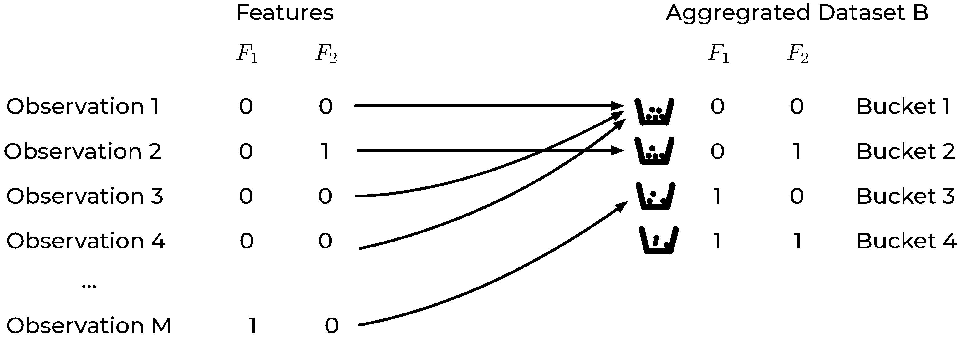
Based on the definitions above, the original dataset can be equivalently represented by a new dataset of buckets, an
aggregated dataset B, each of which contains a certain number of samples
. A visual representation of the previously described rearrangement of the original dataset is reported in
Figure 1 for a dataset with two binary features.
In the aggregated dataset
B, each record is thus a feature bucket
, characterized by the number of observations of class 0 (
) and the number of observations of class 1 (
). In the previous example of a dataset with only two binary features,
B would look like the one in
Table 1. In this easy example a dataset with any number of observations
M would be reduced to one with only 4 records, i.e., the number of possible buckets.
With this new representation of the dataset, generated by aggregating all observations sharing the same feature values in buckets, the proposed ILD algorithm allows computing the best possible ROC curve considering all possible predictions.
3. ILD Algorithm Mathematical Framework
As the output of any machine learning model is a function of the feature values, and as a bucket is a collection of observations all with the same feature values, any possible deterministic model will associate to the jth bucket of features only one possible class prediction that can be either 0 or 1. More in general, to each model can be associated a prediction vector . In the next sections important quantities (as TPR and FPR) evaluated for the aggregated dataset B as functions of , and are derived.
3.1. True Positive, True Negative, False Positive, False Negative
In the feature bucket
i, if
, then only
observations would be correctly classified. On the other side, if
, only
observations would be correctly classified. For each bucket
i the true positive
can be written as
In fact, if
, then
, and if
, then
. Considering the entire dataset, the true positive, true negative (
), false positive (
), false negative (
) are given by
where the sums are performed over all the
buckets.
3.2. Accuracy
In a binary classification problem, the accuracy is defined [
22] as
Using Equations (
7) and (
8), the accuracy can be rewritten as
The maximum value of the accuracy is obtained if the model predicts as soon as . This can be stated as
Theorem 1. The accuracy for an aggregated categorical dataset B, expressed as Equation (12), is maximized by choosing when and when . Proof. The proof is given by considering each bucket separately. Let’s consider a bucket
i that has
. In this case, there are two possibilities:
Therefore, the
ith contribution to the accuracy in Equation (
12) is maximized by choosing
for those buckets where
. With a similar reasoning, the contribution to the accuracy for those buckets where
is maximized by choosing
. This concludes the proof. □
3.3. Sensitivity and Specificity
The sensitivity or true positive rate (
) is the ability to correctly predict the positive cases [
22]. Considering the entire dataset, the
can be expressed using Equations (
7) and (
10) as
Analogously, the specificity or true negative rate (
), which is the ability to correctly reject the negative cases [
22], can be written using Equations (
8) and (
9) as
3.4. ROC Curve
The receiver operating characteristic (ROC) curve is built by plotting the true positive rate
on the
y-axis, and the false positive rate (
) on the
x-axis. For completeness, the
is
3.5. Perfect Bucket and Perfect Dataset
Sometimes a bucket may contain only observations that are all in class 0 or 1. Such a bucket is called in this paper perfect bucket and is defined as follows.
Definition 3. A feature bucket j is called perfect if one of the following is satisfied:or It is also useful to define the set of all perfect buckets P.
Definition 4. The set of all perfect buckets, indicated with P is defined by
Note that by definition, the set contains only imperfect buckets, namely, buckets where and .
An important special case is that of a
perfect dataset, one in which all buckets are perfect. Indicating with
B the set containing all buckets, we have
. It is easy to see that we can create a prediction vector that will predict all cases perfectly, by simply choosing, for feature bucket
jRemember that all feature buckets are perfect, and in a perfect feature bucket and cannot be greater than zero at the same time. To summaries our definitions we can define the following.
Definition 5. A dataset B (where B is the dataset containing all feature buckets) is called perfect if .
Definition 6. A dataset B (where B is the dataset containing all feature buckets) is called imperfect if .
4. The Intrinsic Limit Determination Algorithm
Let us introduce the predictor vector
, for which it clearly holds
and indicate and evaluated for , respectively.
Let us indicate as a
flip the change of a component of a prediction vector from the value of 1 to the value of 0. Any possible prediction vector can thus be obtained by a finite series of flips starting from
, where a flip is done only on components with a value equal to 1. Let us denote with
the prediction vector obtained after the first flip,
after the second, and so on. After
flips, the prediction vector will be
. The
and
evaluated for a prediction vector
(with
) are indicated as
and
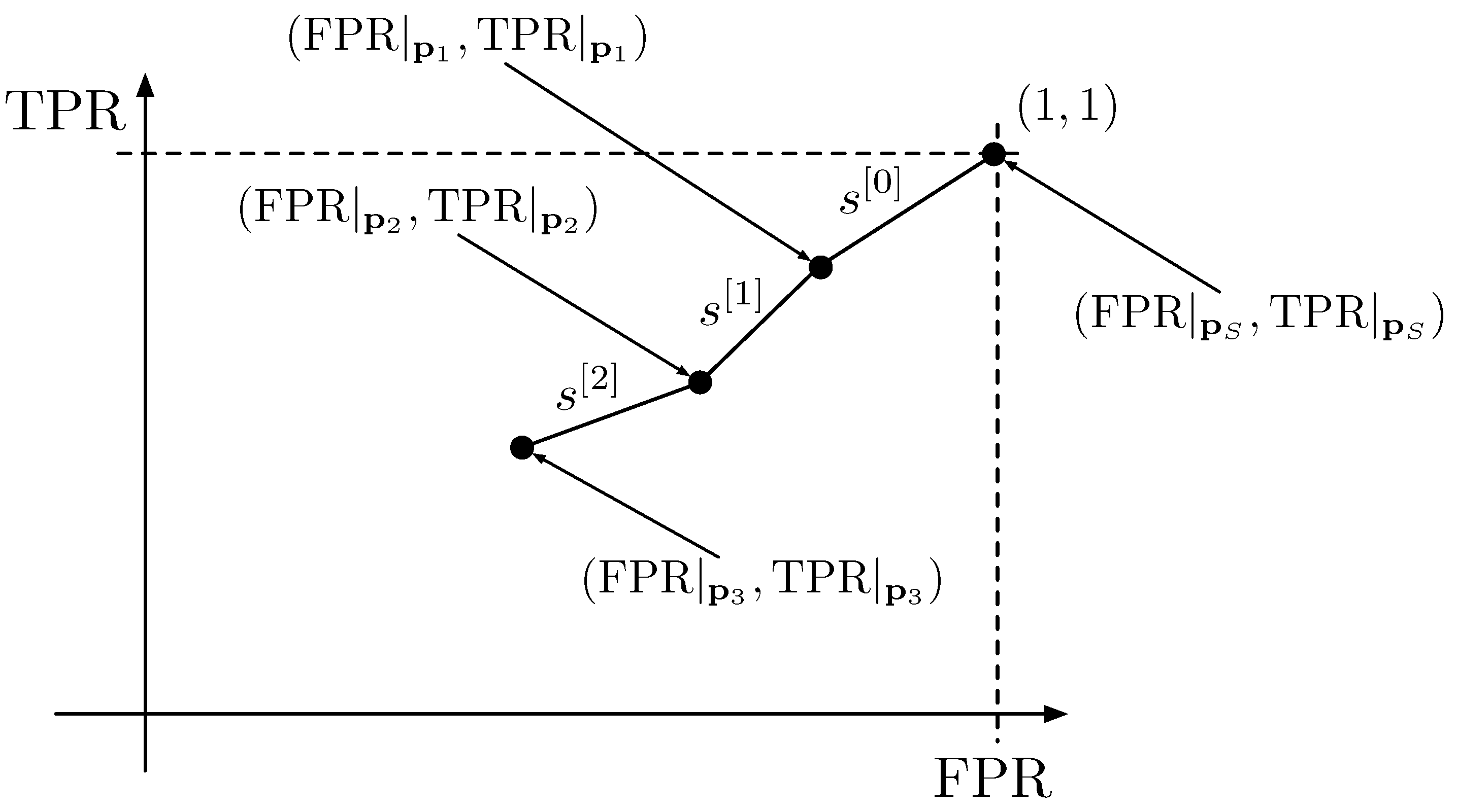
. The set of tuples of points’ coordinates is indicated with
:
A curve can be constructed by joining the points contained in
in
ordered segments, where ordered segments means that the point
will be connected to
;
with
; and so on. The segment that joins the point
with
is denoted as
; the one that joins the points
and
is denoted as
, and so on. In
Figure 2, a curve obtained by joining the tuples given by the respective prediction vectors obtained with three flips is visualized to give an intuitive understanding of the process.
The ILD algorithm provides a constructive process to select the order of the components to be flipped to obtain the curve characterized by the theoretical maximum AUC that can be obtained from the considered dataset, regardless of the predictive model used.
To be able to describe the ILD algorithm effectively and prove its validity, some additional concepts are needed and described in the following paragraphs.
4.1. Effect of One Single Flip
Let us consider what happens if one single component, say the
jth component, of
is changed from 1 to 0. The
and
values clearly change. By denoting with
the prediction vector in which the
jth component was changed, the following equations hold:
Therefore,
and
will be reduced by an amount equal to the ratio
and
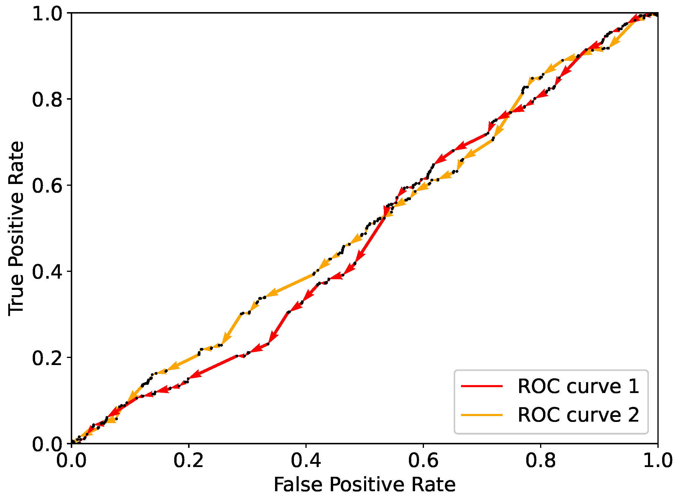
, respectively. As an example, the effect of multiple single flips on
and
is illustrated in
Figure 3. Here are shown the ROC curves resulting from a random flipping starting from
for a real-life dataset, namely, the Framingham dataset [
23] (see
Section 5). As expected, flipping components randomly results in a curve that lies close to the diagonal. As the diagonal corresponds to randomly assigning classes to the observations, randomly flipping does not bring to the best prediction possible with the given dataset.
By ordering the points in in ascending order based on the ratio , a new set of points is constructed. It can happen that in a given dataset, multiple points have . In this case, this ratio cannot be calculated. If this happens, all the points with can be placed at the end of the list of points. The order between those points is irrelevant. It is interesting to note that a flip for perfect buckets for which will have and for all perfect buckets for which will have .
With the set of ordered points , a curve can be constructed by joining the points in as described in the previous paragraph. Note that the relative order of all points with is also irrelevant, in the sense that this order does not affect the AUC of .
4.2. ILD Theorem
The ILD theorem can now be formulated.
Theorem 2 (ILD Theorem). Among all possible curves that can be constructed by generating a set of points by flipping all components of in any order one at a time, the curve has the maximum AUC.
Proof. The Theorem is proven by giving a construction algorithm. It starts with one set of points
generated by flipping components of
in a random order. Let us consider two adjacent segments generated with
:
and
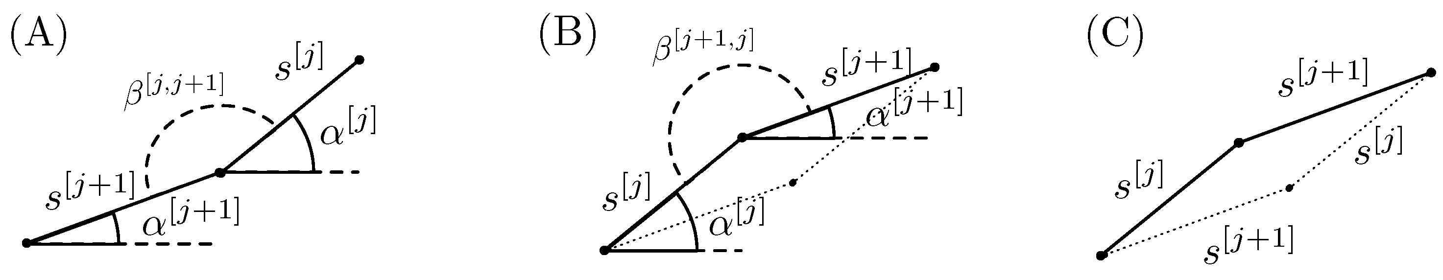
. In
Figure 4A, the two segments are plotted in the case where the angle between them
. The angles
and
indicate the angles of the segments with the horizontal direction and
the angle between the two segments
j and
. The area under the two segments and any horizontal line that lies below the segments can be increased by simply switching the order of the two flips, as it is depicted in
Figure 4B. Switching the order simply means flipping first the
component and then the
j component.
It is important to note that in
Figure 4A
, while in panel (B)
. It is evident that the area under the two segments in panel (B) is greater than the one in panel (A). The parallelogram in
Figure 4C depicts the area difference.
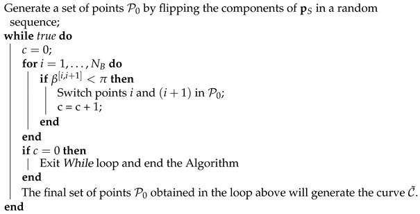
The proof is based on repeating the previous step until all angles . This is described in pseudocode in Algorithm 1.
| Algorithm 1: to construct the curve |
![Algorithms 14 00301 i001]() |
The area under the curve obtained with Algorithm 1 cannot be made larger with any further switch of points in . □
Note that Algorithm 1 will end after a finite number of steps. This can be shown by noting that the described algorithm is nothing else than the bubble sort algorithm [
24] applied to the set of angles
,
, ...,
. Therefore, this algorithm has a worst-case and average complexity of
.
4.3. Handling Missing Values
Missing values can be handled by imputing them with a value that does not appear in any feature. All observations that have missing values in a specific feature will be assigned to the same bucket and considered similar, as we have no way of knowing better.
5. Application of the ILD Algorithm to the Framingham Heart Study Dataset
In this section, a practical application of the ILD algorithm is illustrated. The application to a real dataset has the purpose of giving an intuitive understanding of the method and highlight its power. Here, the medical dataset named Framingham [
23] were chosen, which is publicly available on the Kaggle website [
25]. This dataset comes from an ongoing cardiovascular risk study made on residents of the town of Framingham ( Framingham, MA, USA). Different cardiovascular risk score versions were developed during the years [
26], the most current of whom is the 2008 study in [
27], to which the ILD algorithm results are also referred for comparison of performances. The reader interested in descriptive statistics on the dataset’s features (averages, standard deviations, counts, description, etc.) can find all information in [
23].
The classification goal is to predict, given a series of risk factors, the 10-years risk of a patient of future coronary heart disease. This is a high impact task, as 17.9 million deaths occur worldwide every year due to heart diseases [
28] and their early prognosis may be of crucial importance for a correct and successful treatment. Note that the dataset available in [
25] has 16 features. To make the comparison as meaningful as possible, seven of the eight features used in the original study [
23] were selected. The high-density lipoprotein (HDL) cholesterol variable is unfortunately missing with respect to the original Framingham dataset employed in [
27] and therefore could not be used. Thus, the dataset used in this study contains 4238 patients and 7 features: gender (0: female, 1: male); smoker (0: no, 1: yes); diabetes (0: no, 1: yes); hypertension treatment (0: no, 1: yes); age; total cholesterol; and systolic blood pressure (SBP). The last three features are continuous variables and were discretized as follows:
age: ;
total cholesterol: ;
SBP: .
The outcome variable is binary (0: no coronary disease, 1: coronary disease). Finally, to create the buckets all missing values are substituted by a feature value of −1.
The application of the algorithm starts with the population of the buckets as described in the previous sections. A total number of 177 buckets are populated. The dataset is split into two parts: a training set
(80% of the data) and a validation one
(20% of the data). For comparison, the Naïve Bayes classifier is also trained and validated respectively on
and
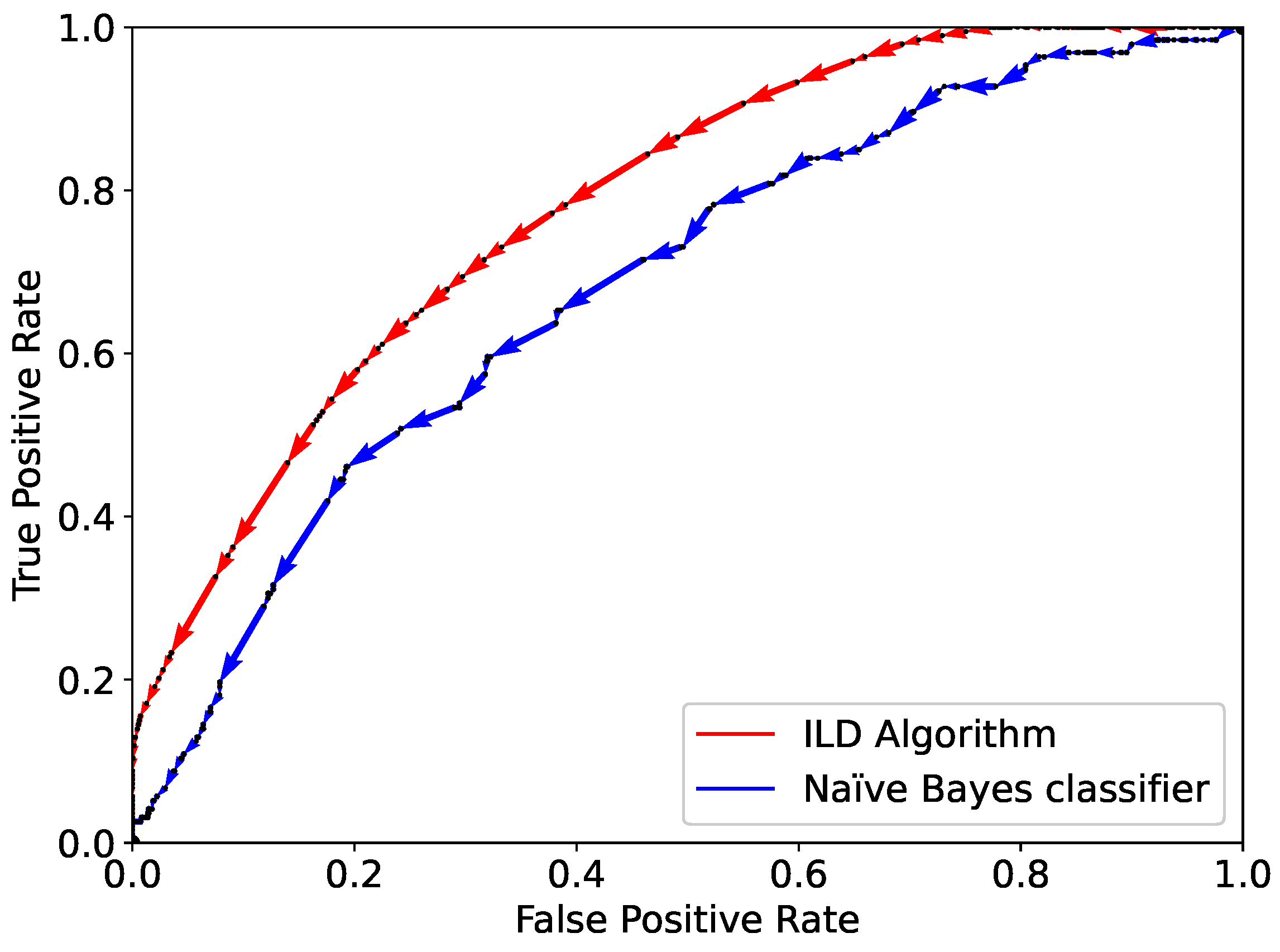
. The performance of the ILD algorithm and the Naïve Bayes classifier are shown through the ROC curve in
Figure 5. The AUC for the ILD algorithm is 0.78, clearly higher than that for the Naïve Bayes classifier, namely, 0.68.
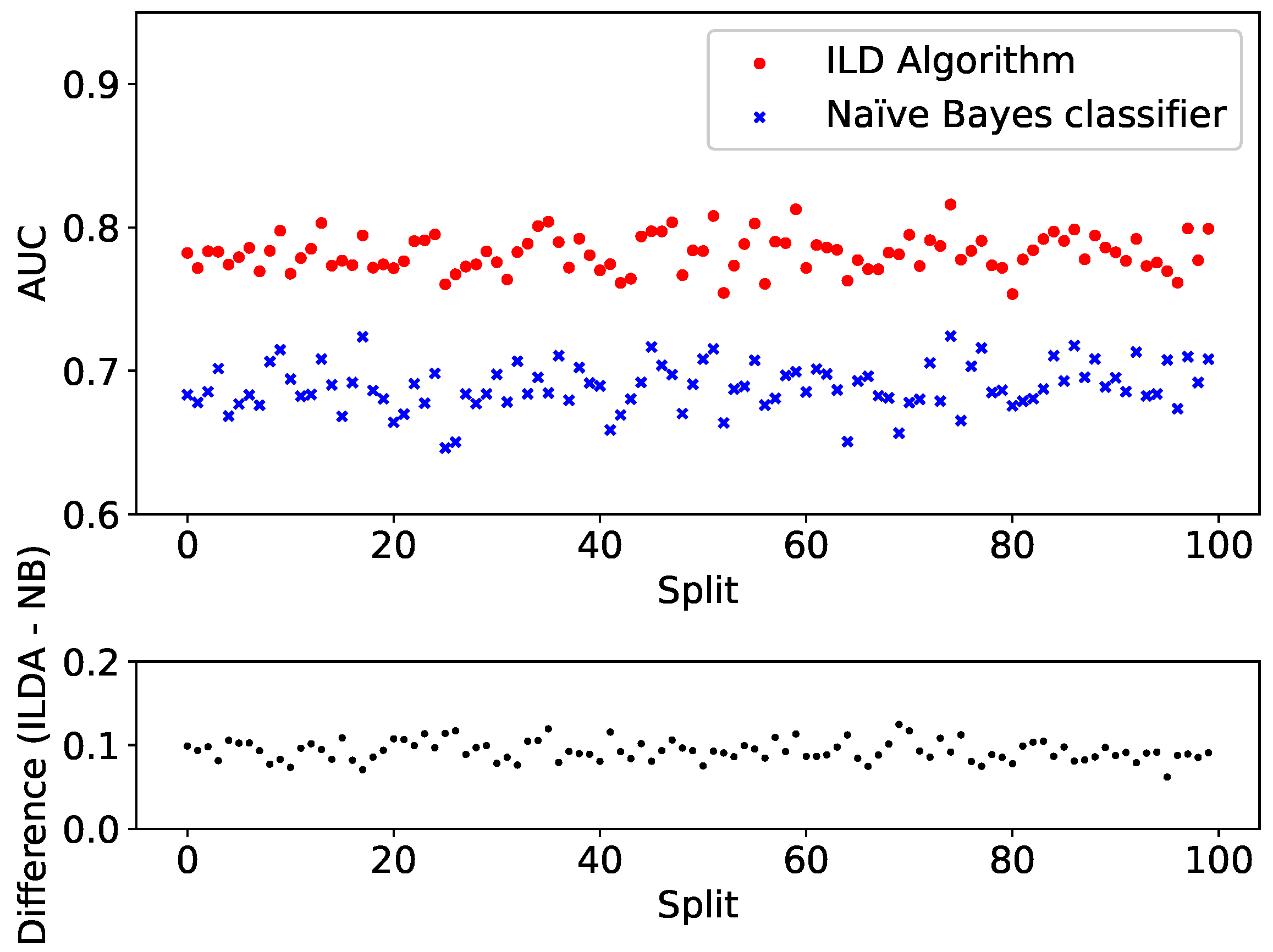
To further test the performance, the split and training is repeated for 100 different dataset splits. Each time both the ILD algorithm and the Naïve Bayes classifier are applied to the validation set
and the resulting AUCs are plotted in
Figure 6 (top panel). For clarity, the difference between the AUC provided by the two algorithms is shown in
Figure 6 (bottom panel).
This example shows that the application of the ILD algorithm allows the comparison of the prediction performance of a model, here the Naïve Bayes classifier, with the maximum obtainable for a given dataset. The maximum accuracy over the validation set
is 85% for the Naïve Bayes classifier (calculated for a specific threshold, i.e., 61%, which optimizes the accuracy over the training set
) and 86% for the ILD algorithm (calculated applying Theorem 1). The reported accuracies are the ones that refer to the ROC curves shown in
Figure 5. The two values are similar and have been reported for completeness, even if this result may by misleading. The reason lies in the strong dataset unbalance, as only 15% of the patients experienced a cardiovascular event. In particular, both the Naïve Bayes classifier and ILD algorithm obtains a true positive rate and a false positive rate near zero in the point of the ROC curve which maximises the accuracy over the validation set, with a high misclassification in positive patients, which however cannot be noticed from the accuracy result. As it is known, the accuracy is not a good metric for unbalanced datasets, and the AUC is a much widely used metric that does not suffer from the problem described above.
The authors are aware that this is an unbalanced dataset and that balanced datasets are easier to deal with when studying classification problems. The goal was to give an example that reflects real use cases. For example, in medical problems, datasets are almost always extremely unbalanced since the event to be predicted is thankfully rare (for example death or the onset of diseases). It is not uncommon to find datasets with an unbalance of 99% vs. 1%. This was also the reason why the ILD algorithm concentrates on the AUC, as this is the typical metric used when dealing with such use-cases.
6. Conclusions
The work presents a new algorithm, the ILD algorithm, which determines the best possible ROC curve that can be obtained from a dataset with categorical features and binary outcome, regardless of the predictive model.
The ILD algorithm is of fundamental importance to practitioners because it allows:
to determine the prediction power (namely, the BE) of a specific set of categorical features,
to decide when to stop searching for better models, and,
to decide if it is necessary to enrich the dataset.
The ILD algorithm thus has the potential to revolutionize how binary prediction problems will be solved in the future, allowing practitioners to save an enormous amount of efforts, time, and money (considering that, for example, computing time is expensive especially in cloud environments).
The limitations of the ILD algorithm are the two restrictions for its applicability. First, the features must be categorical. The generalization of this approach to continuous features is the natural next step and will open new ways of understanding datasets with continuous features. Second, the ILD algorithm works well when the different buckets are populated with enough observations. The ILD algorithm would not give any useful information on a dataset with just one observation in each bucket (as it would be a perfect dataset). Consider the example of gray levels images. Even if pixel values could be considered categorical (the gray level of a pixel is an integer that can assume values from 0 to 255), two major problems would arise if the ILD algorithm would be applied to such a case: the number of buckets would be extremely large and each bucket would contain only one image therefore making the ILD algorithm completely useless, as only perfect buckets will be constructed.
An important further research direction is the expansion of the ILD algorithm to detect the best performing models that do not overfit the data. In the example of images, it is clear that being a perfect dataset one could theoretically construct a perfect predictor, therefore giving a maximum accuracy of 1. The interesting question is how to determine the maximum accuracy or the best AUC only in cases in which no overfitting is occurring. This is a nontrivial problem that is currently under investigation by the authors. To address, at least partially, this problem, the authors have defined a perfection index (IP) that can help in this regard. IP is discussed in
Appendix A.
It is useful to note that this method differs significantly from other works as, for example, that in [
29], where the authors describes RankOpt, a linear binary classifier which optimizes the area under the ROC curve (the AUC) or that in [
30], which presents a Support Vector Method for optimizing multivariate nonlinear performance measures like the F1-score. This method is completely model-agnostic (in other words it does not depend on any model type) and determines the absolute maximum of the AUC with the given datasets. It does not try to maximize it, but it finds its absolute maximum.
To conclude, although more research is needed to generalize the ILD algorithm, it is, to the best knowledge of the authors, the first algorithm that is able to determine the exact BE from a generic dataset with categorical features, regardless of the predictive models.


 ,
, 


