Article

Research on Building Target Detection Based on High-Resolution Optical Remote Sensing Imagery

1
Institute of Defense Engineering, AMS, Beijing 100036, China
2
School of Electronics and Information Engineering, Harbin Institute of Technology, Harbin 150006, China
*
Author to whom correspondence should be addressed.
Algorithms 2021, 14(10), 300; https://doi.org/10.3390/a14100300
Submission received: 2 October 2021 / Revised: 14 October 2021 / Accepted: 15 October 2021 / Published: 19 October 2021
(This article belongs to the Special Issue Machine Learning in Image and Video Processing)

Abstract

:
High-resolution remote sensing image building target detection has wide application value in the fields of land planning, geographic monitoring, smart cities and other fields. However, due to the complex background of remote sensing imagery, some detailed features of building targets are less distinguishable from the background. When carrying out the detection task, it is prone to problems such as distortion and the missing of the building outline. To address this challenge, we developed a novel building target detection method. First, a building detection method based on rectangular approximation and region growth was proposed, and a saliency detection model based on the foreground compactness and local contrast of manifold ranking is used to obtain the saliency map of the building region. Then, the boundary prior saliency detection method based on the improved manifold ranking algorithm was proposed for the target area of buildings with low contrast with the background in remote sensing imagery. Finally, fusing the results of the rectangular approximation-based and saliency-based detection, the proposed fusion method improved the Recall and F1 value of building detection, indicating that this paper provides an effective and efficient high-resolution remote sensing image building target detection method.

Graphical Abstract

1. Introduction

Accurate building target detection has important scientific and practical significance in urban 3D modeling and urban dynamic change management. The problem of building target detection has been a research hotspot in the field of remote sensing; however, timely and accurate detection of building targets on high-resolution remote sensing images is a challenge. With the development of remote sensing technology, the spatial resolution of optical remote sensing images has been gradually improved, and nowadays it has entered the sub-meter level, and the related research on remote sensing images has become an important part of the field, providing unprecedented opportunities for the development of remote sensing applications [1,2,3].
Building target detection based on remote sensing images has been developed rapidly with the development and popularization of remote sensing technology [4,5,6]. At present, the research on building detection based on remote sensing images at home and abroad can be mainly divided into three types of methods based on geometric structure, supervised classification and texture features.
Compared with the non-building backgrounds, the building targets have relatively regular geometric structures, and their geometric features are the most obvious and typical characteristics of buildings, which are inherent properties not easily affected by changes in external temperature, humidity, and light. Therefore, geometric structure-based detection methods are one of the most popular methods in the research of building detection. Mi et al. [7] used Scale Invariant Feature Transform (SIFT) (in Table A1) and adaptive windowed Hoff transform to extract the corner points of building targets and the line segments forming the boundary for detection. Zhang et al. [8] proposed a building detection method for very high spatial resolution (VHR) images based on the classical local binarization algorithm. The geometric structure-based approach is popular for research. It takes advantage of the fact that the basic structure of the building target is composed of a rectangle of different shapes, so it adopts the detection of right angles, line segments or corner points of the rectangular structure to extract features such as point, line, surface features and gradient features of the building, and then realize the detection of the building.
With the rapid development and application of deep learning, there are more and more examples of deep learning algorithm applications in building detection, including YOLO series, CNN, ImageNet, DeconvNet and many other algorithms. Vakalopoulou et al. [9] used a very large training dataset for supervised classification, using powerful CNNs and a huge pre-trained ImageNet to extract buildings, with good quantitative validation results, but high difficulty and huge time consumption to obtain the training dataset. Zhang et al. [10] proposed a method for automatic detection of suburban buildings based on super-scale saliency sliding window detection of candidate regions combined with CNNs. Liu et al. [11] proposed a hierarchical building detection framework based on deep-learning models. The Gaussian pyramid technique is used to construct a generative model of multi-layer training samples, and a building area suggestion network is proposed to quickly extract candidate building areas. Convolutional neural networks (CNNs) are used to build a multi-layer building detection model for detecting building targets in remote sensing images. The advantages of the deep-learning-based approach are high accuracy and ease of use, while the disadvantages are high difficulty in obtaining training datasets and high time consumption.
Texture features contain image color, contrast, gray-scale histogram, gray-scale co-occurrence matrix, all of which are very important information for the target detection process of remote sensing images. Sidike et al. [12] proposed an adaptive local texture feature detection method based on continuous background removal. Manandhar et al. [13] proposed to extract buildings based on contextual and spectral difference segmentation. First, a single-class support vector machine (SVM) is used to determine artificial structures, such as buildings, roads, and then a conditional threshold is used for texture segmentation to extract buildings, and finally noise, vegetation and shadows are removed from the candidate building areas.
Currently, the basic concept of optical remote sensing image building target detection research is to use feature differences, that is, the geometric structure, color, contrast and spectral characteristics of the building target itself to separate the building target from the background, but when applied to remote sensing images with low resolution, or when the contrast between the building area and the background area in the image is low, most of the methods are difficult to maintain a strong applicability. Local occlusion of buildings, different lighting conditions, and different types of interference, such as stacks, ships, playgrounds, and flower beds, all seriously affect the detection results. Moreover, most of the methods aim to detect the top surface of the building target, which is difficult to detect when there is a silhouette of the building target in the image. The existing building target detection methods, deep learning-based building detection methods are more widely used. Among them, the pixel-based classification and recognition methods can hardly consider the neighborhood information around the pixels, so the contours of buildings cannot be well guaranteed. The existing wavelet transform-based building detection methods, which is difficult for the detection of complex building backgrounds and the study of complex building roofs. Combining the above problems and shortcomings, it is important to study building detection techniques that resist low contrast between building targets and background, detect the contours of building targets, and remove various types of interference.
The remainder of this paper is organized as follows. Section 2 introduces the experimental data used in this work, details the specific workflow of research, including building detection based on rectangular approximation and region growing, building detection based on multi-feature saliency, fusion of the rectangular approximation-based and saliency-based detection results, and evaluation. Section 3 is a comparative analysis of experimental results. Discussions and conclusions are presented in Section 4 and Section 5, respectively.

2. Data and Methodology

2.1. Data

The details of the data used for the experiments are shown in Table 1 and Table 2. This experiment used the Jilin-1 Gaofen 03-1 satellites with a spatial resolution of 1 m, and the image acquisition date is 11 October 2020. The study area is located in Yokosuka, Japan. Four representative images were intercepted from the original image for experimentation.
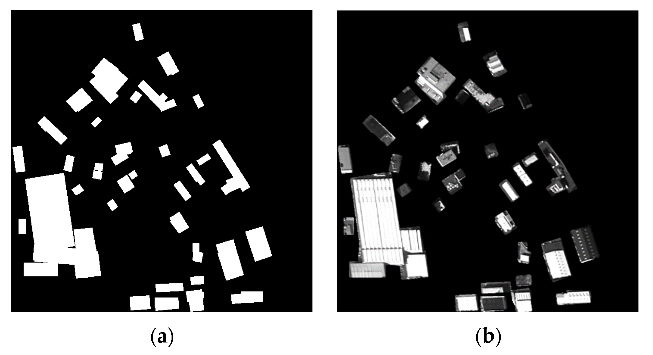
The optical remote sensing images used in this experiment and the corresponding ground truth maps are shown in Figure 1.

2.2. Methodology

This paper focuses on the research of building target detection based on optical remote sensing images. First, since the common components of a typical geometric structure of the vertical top view of a building are right-angle primitives composed of mutually perpendicular line segments, right-angle primitives are obtained using the broken line segment connection method and the right-angle detection method based on voting strategy. Then, the inner and outer corners are classified to achieve multiple shapes of building top surface detection, and finally the complete top surface area of the building is obtained by using the image segmentation algorithm based on region growth. However, detection by shape features only can lead to problems such as incomplete detection of the building target facade area and inaccurate results caused by light occlusion. Therefore, the compactness and local contrast-based saliency model of the manifold ranking algorithm is introduced, while considering the low contrast between the building target areas and the background in remote sensing images, and then using the boundary priori saliency detection of the improved manifold ranking algorithm. The bounding box proposal is introduced to remove the environmental noise, and finally the final saliency map is obtained by integrating each detection result and setting the adaptive threshold to obtain the mask map. The rectangular approximation-based and the saliency-based detection results are fused and the interference in the ocean area is removed to obtain the final detection results. In this paper, the unbold notations represent scalars, the lowercase boldface letters represent vectors, and the uppercase boldface letters represent matrices.

2.2.1. Building Detection Based on Rectangular Approximation and Region Growth

The geometric structure of a typical vertical top view of a building, including L-shaped building, concave building, rectangular building and cross-shaped building, has a common component of right-angle primitives composed of mutually perpendicular line segments, and the extraction of such right-angle primitives with the rectangular approximation technique based on right-angle primitives can better extract buildings with different vertical top views of geometric structures. Figure 2 presents the flowchart of the algorithm used in this study.
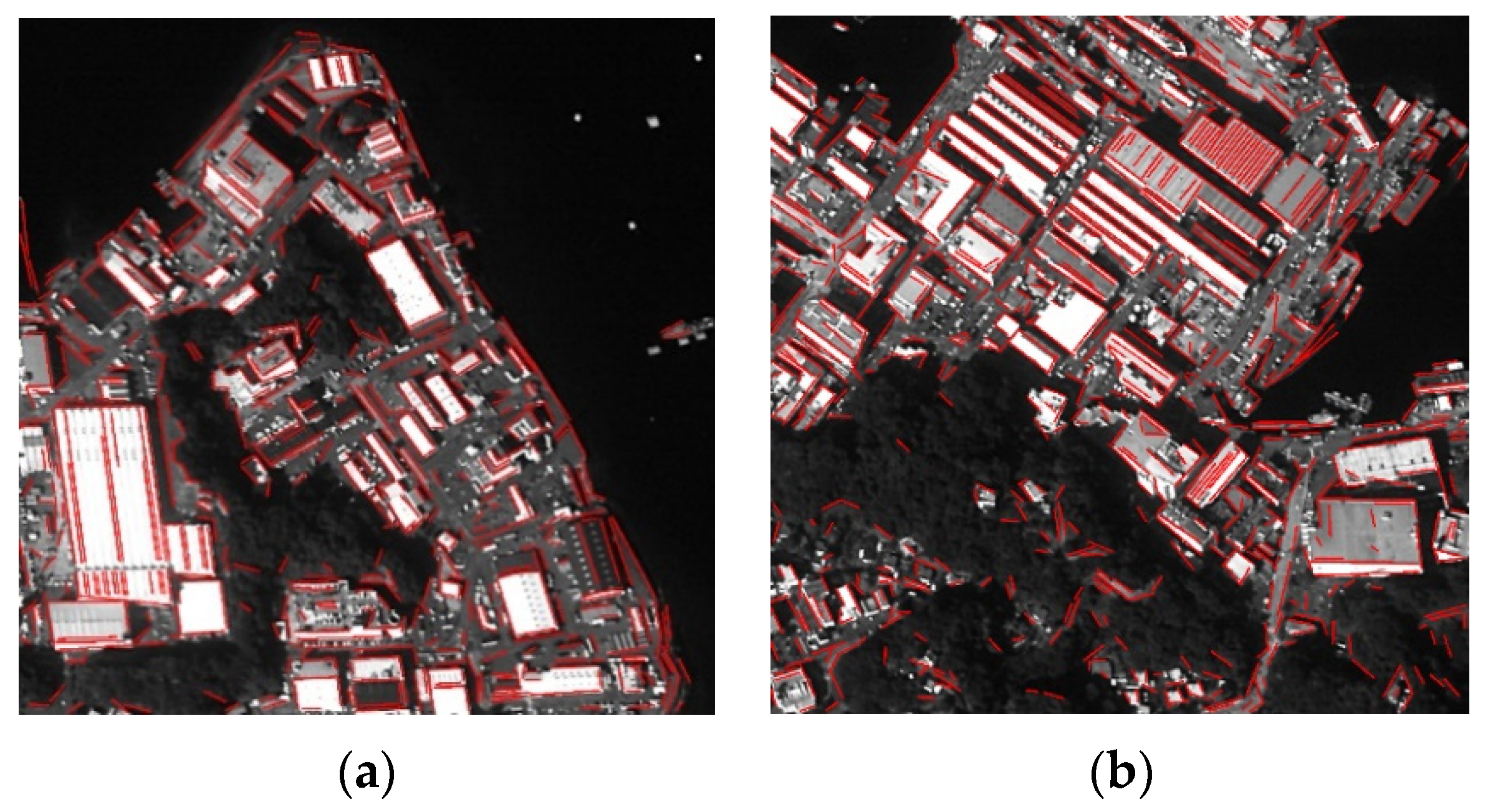
Extracting right-angle primitives of buildings requires the detection of line segments in remote sensing images. The LSD-based line segment detection method has a faster extraction speed and has been successfully applied in airport detection and the road detection of remote sensing images. For this purpose, the line segments of remote sensing images are extracted using the LSD [14] method, and the line segment detection results are shown in Figure 3.
The results of LSD show that the extracted line segments are fractured at the point where the gradient changes strongly. In order to prevent the fracture of the boundary line of the building from adversely affecting the building detection results, a fractured line segment connection method is constructed to optimize the LSD detection results.
Connectable broken line segments satisfy the approximate covariance as well as the small distance in the direction of covariance. Based on these two properties, the following criterion can be constructed to discriminate whether all straight-line pairs are broken pairs.
l i , l j l i 2 l j 2 δ 1
d i 1 d j 1 , ( c i c j ) ( c i c j ) 2 δ 2
min k , m { 1 , 2 } ( d i k d j m , c i c j c i c j 2 ) δ 3 ,
where l i , l j , d i 1 , d j 1 , c i , c j are the vector of the ith and the jth line segments, the coordinates of the endpoint 1 of the ith and the jth line segments, the coordinates of the midpoint of the ith and the jth line segments, respectively. k , m { 1 , 2 } represents endpoint 1 or endpoint 2 of the line segment, and δ 1 , δ 2 , δ 3 are the threshold values.
The first discriminant indicates the cosine of two line segments, that is, line segment parallelism detection. ( c i c j ) indicates the zero space of ( c i c j ) . The second discriminant indicates the projection of the distance of the endpoints of the line segment in the ( c i c j ) direction is less than the threshold, that is, line segment co-linearity detection. The third discriminant indicates the projection of the line segment composed of any endpoints of two line segments in ( c i c j ) is less than the threshold, that is, line segment break length discrimination.
The above three discriminatory formulae are parallelism, covariance and fracture distance discriminations, and the current line segment pair is connected if the above conditions are satisfied. Removing vehicles and other interfering line segments further improves the accuracy of subsequent building target extraction and reduces the computational effort.
We construct a right-angle primitive extraction method to detect the right-angle primitives of buildings. Given that the mutually perpendicular line segments of buildings in remote sensing images may not be adjacent, the right-angle primitive detection method needs to be ambiguous to tolerate the case of non-adjacent perpendicular line segments. A position-angle voting space V R M × N × A is created for extracting potential right-angle primitives, where M is the number of rows of the image, N is the number of columns of the image, and A is the number of intervals of the angle. For each straight-line segment l , the neighboring entrances centered at each endpoint at the corresponding entrance of the position angle voting space are voted simultaneously as shown in Equation (4).
V ( i + τ , j + τ , α + τ ) = V ( i + τ , j + τ , α + τ ) + 1     ε τ ε ,
where i , j and α are the row and column coordinates of an endpoint of the line segment and the direction of the line segment, respectively. The line segment direction can be calculated simply using the inverse cosine, which is shown in Equation (5).
α = r o u n d ( arccos ( l i , β l i 2 ) / Δ α ) ,
where β is the horizontal unit vector and Δ α is the angular interval. After traversing all the line segments, the potential right-angle primitives are extracted using the following Equation (6).
R = V & V × 3 F F ( i , j ) = { 1   i f   | j i | = A / 2 0   o t h e r w i s e
where F is the shift matrix, R is the right-angle primitive detection result, × 3 represents the third dimension of V is multiplied by F , and A is the number of intervals of the angle.
For a typical L-shaped and cross-shaped building, the endpoints of the right-angle edges of the outer corners of the building are dependent on the two inner corners of the building and are oriented in the opposite direction to the right-angle primitives of the outer corners. Using this feature, all right-angle primitives in the voting space are traversed, and whether the right-angle primitive is the building outer corner primitive is determined by Equation (7).
max { α α 1 , α α 2 } δ ,
where α is the right-angle primitive to be identified, α 1 and α 2 are the right-angle primitives at the endpoints of the right-angle edges of the primitive, and δ is the outer-angle threshold. If the above conditions are satisfied, then α is considered to be an exterior right-angle primitive, otherwise α is an interior right-angle primitive.
Based on the final right-angle primitive extraction results, a rectangular region can be obtained using the right-angle and the two sides enclosing the right-angle, which can be considered as the building region.
Since the studied building targets include L-shaped buildings, concave buildings, rectangular buildings and cross-shaped buildings, a single rectangular approximation can only obtain a local area of the building top surface. In order to obtain the complete building top surface, we combine the similar spectral characteristics of the building top surface, extract the seed points in the rectangular area formed by the right-angle edges, and use the proposed restricted region growth algorithm to obtain complete building top surface. The specific steps are as follows.
Step 1: Extract the seed points contained in the right-angle edges.
Step 2: The larger rectangular area enclosed by the extensions of the right-angled edges is used as the maximum growth region.
Step 3: Execution of region growth algorithm.
The complete segmentation of the building is achieved using the region growing algorithm to obtain the final detection results.

2.2.2. Diffusion-Based Saliency Model

In order to improve the accuracy of building detection and reduce missed detection and misjudgment, the saliency model is used for building target detection. The specific flowchart is shown in Figure 4.
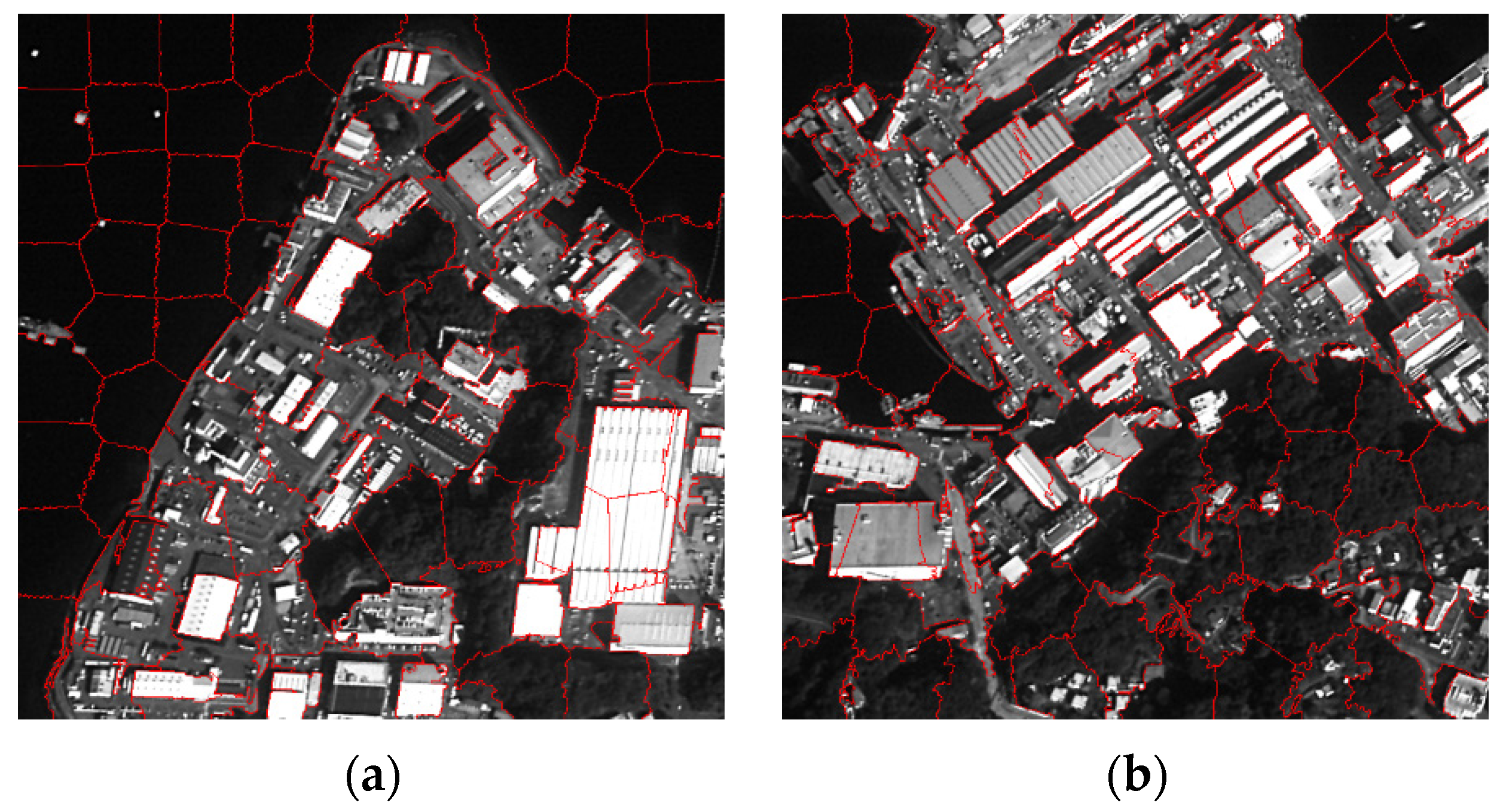
In order to improve the accuracy of building detection and reduce missed detection and misjudgment, the saliency model is used for building target detection. The specific flowchart is shown in Figure 4. First, the SLIC super-pixel segmentation method is used. This method uses the K-means algorithm to generate the super-pixels, and the color values and spatial distances of the images together define the distance metric function used for clustering. The results of super-pixel segmentation are shown in Figure 5.
After generating the SLIC super-pixel model, a construction graph G = (V,E) is obtained, where V represents the node, E represents the undirected edge connecting the nodes, and the saliency values of adjacent nodes are very similar with high probability. And any two boundary nodes of the construction graph are adjacent to each other, thus forming a closed-loop graph, which can effectively reduce the geodesic distance of similar super-pixels, and then optimize the ranking results of the manifold ranking algorithm.
Assuming that N i denotes the set of neighboring points of node v i , and all nodes around the image boundary are considered as neighboring points of each other. Calculate the distance between the nodes in the CIELab color space, that is, the difference between the mean values of the superpixels corresponding to the two nodes and normalize them to obtain the incidence matrix W and use manifold ranking algorithm to achieve saliency propagation.
The tightness of the super-pixel blocks is defined by the degree of similarity between super-pixel blocks and spatial location, and to describe the similarity between super-pixels more precisely, define A = [ a i j ] N × N as the color similarity metric between a pair of super-pixels v i and v j , where a i j = exp ( c i c j / σ 2 ) , and use the manifold ranking algorithm to propagate the similarity between super-pixels to obtain H T = ( D α W ) 1 A , where the computed result H = [ h i j ] N × N is the executed diffusion of the similarity metric matrix. The method for calculating the spatial variance of the super-pixel v i is shown in Equation (8).
s v ( i ) = j = 1 N h i j n j b j u i j = 1 N h i j n j ,
where n j is the number of pixels of super-pixel v j and b j = [ b j x , b j y ] is the center of mass of super-pixel v j and defines the spatial mean μ i = [ μ i x , μ i y ] as Equation (9).
μ i x = j = 1 N h i j n j b i x j = 1 N h i j n j μ i y = j = 1 N h i j n j b i y j = 1 N h i j n j
The saliency map calculated by the diffusion-based foreground compactness saliency [15] detection method is shown in Equation (10).
S c o m ( i ) = 1 N o r m ( s v ( i ) ) ,
where Norm(.) is the function that normalizes the data to 0–1.
Define the Lab color space distance l d ( i ) of the super-pixel v i and its neighboring super-pixels as Equation (11).
l d ( i ) = j N i S c o m ( j ) n j j N i n j max j N i c i c j .
The smaller the value of l d ( i ) , the higher the probability that the super-pixel v i belongs to the background. The ld value smaller than the ld mean is set to 0. To improve the reliability of foreground detection and the overall quality of the saliency region segmentation, the distribution metric of super-pixel v i relative to the center of mass of the compactness-based saliency map S c o m is defined as Equation (12).
d m ( i ) = j = 1 N m i j n j b j u s j = 1 N m i j n j ,
where m i j is the spatial distance similarity measure of a pair of super-pixels v i and v j , defined as m i j = a i j exp ( b i b j / σ 2 ) . μ s = [ μ s x , μ s y ] is the center of mass of the compactness-based saliency map S c o m . u s is calculated in the same way as Equation (9).
μ s x = i = 1 N S c o m ( i ) n i b i x i = 1 N S c o m ( i ) n i μ s y = i = 1 N S c o m ( i ) n i b i y i = 1 N S c o m ( i ) n i
Combining the Lab color space distance ld and the distribution metric dm to define the local contrast, the N-dimensional column vector lc is obtained, as shown in Equation (14).
l c ( i ) = l d ( i ) ( 1 N o r m ( d m ( i ) ) ) .
The local contrast lc saliency map [16] tends to highlight the boundaries rather than the entire region. The lc saliency map is propagated using a manifold ranking algorithm to obtain an N-dimensional column vector S l o c = N o r m ( ( D α W ) 1 l c ) .
First, after the image is super-pixel segmented, a preliminary saliency map is generated using the algorithm of Reference [17] with background seeds and a modified manifold ranked diffusion model. The method uses the boundary super-pixel nodes of the experimental image as background seeds to rank the other super-pixel regions. The saliency maps of the four boundary priors are constructed by taking the upper boundary, lower boundary, left boundary and right boundary, respectively. The saliency map using the left boundary prior S l is represented as Equation (15).
S l ( i ) = 1 N o r m ( f ( i ) ) i = 1 , 2 , , N ,
where i is the subscript of the super-pixel node in the experimental image and N o r m ( f ( i ) ) represents the normalized vector of f . Similarly, the saliency map S r for the right boundary prior, the saliency map S t for the top boundary prior, and the saliency map S b for the bottom boundary prior are obtained. The saliency maps of the four boundary priors are integrated to obtain the saliency map: S b q ( i ) = S l ( i ) × S r ( i ) × S t ( i ) × S b ( i ) .
The compactness-based, local contrast-based, and boundary prior-based saliency maps are fused, and the fusion results are shown in Equation (16).
S i n i t = N o r m ( ε c o m S c o m + ε l o c S l o c + ε b d S b d ) ,
where ε represents the weights of the calculation results of the three saliency maps.
In this paper, Edge Boxes proposed in Reference [18] is chosen to generate saliency objects from edges. This algorithm outputs the number of bounding boxes and the score of each bounding box, but the number of generated bounding boxes is large, resulting in a large computational effort. According to Reference [19], the outliers with too large or too small sizes of the bounding boxes are removed, and then the bounding boxes of the regions without high saliency within the boxes are removed. For each super-pixel node, the average score is calculated from the scores of the screened bounding boxes, which is calculated as Equation (17).
m i o = j = 1 Q G j δ ( v i Ω j ) ,
where Q is the number of bounding boxes Ω j , Gj is the score of the bounding box Ω j , and δ ( v i Ω j ) is the indicator function, v i Ω j is 1, otherwise is 0. Get the foreground mask map M o = ( m i o ) N , and calculate d i i o = exp ( m i o ) , D o = ( d i i o ) N × N , with the other elements outside the diagonal as 0.
According to the definition of the construction graph, S i n i t calculates the new degree matrix D c and the new weight matrix W c . Combining M o to obtain the refined saliency map, the refined saliency map is generated by the proposed optimization method in Reference [20].
g = min g 1 2 { g T [ D c W c + μ 2 ( I D c v c ) ] g + g S i n i t 2 + g T D o g } .
The three terms in the formula define different constraint terms. The first two terms correspond to the improved manifold ranking algorithm, the first term is to maintain the continuity of the salient values, so that the detected building target is a whole rather than scattered small areas. The second item is to constrain the difference between the refined saliency map and the saliency map before refinement must not be too large, to maintain the consistency of the detection results, which can play the role of mutual supervision of the two detection results. The third item is to reflect the role of removing the background noise of the bounding box proposal, which can suppress the external environment area that does not belong to the bounding box proposal and highlight the target area of the building.
The optimal solution of Equation (18) is expressed as:
g = [ D c W c + μ 2 ( I D c v c ) + D o ] 1 S i n i t .
The saliency map obtained by combining the bounding box proposal is expressed as:
S f i n a l = N o r m ( g ) .

2.2.3. Pixel-Level Fusion and Interference Removal

The building target detection results based on rectangular approximation and diffusion saliency have been obtained previously, and the two detection results are fused in order to improve the accuracy and recall. In the first two methods of building detection, the screening of detection results is more stringent. The method to fuse the detection results is shown in Equation (21).
R = R r e c R s a l ,
where R r e c represents the mask map generated by the rectangular approximation-based building target detection method and R s a l represents the mask map generated by the multi-feature saliency detection method.
Most of the false alarms in the detected building targets are due to the fact that stacks, various types of ships and vessels in the port area have great similarity in shape and color to the building targets. In order to solve this problem, improve the accuracy of building target detection and reduce false alarms, this paper separates the ocean area from the land area. By observing the remote sensing images, it is found that the image brightness of the water area is lower than that of the land area, which can be used as the basis for segmentation. Use the image segmentation method of region growth to obtain the ocean area. First, the grayscale threshold of the image is calculated by using Otsu algorithm. Then, randomly select the seed points of the sea surface that satisfy Equation (22) [21].
P ( x , y ) = { 1 ( x 1 , y 1 ) U ( x , y ) , I ( x 1 , y 1 ) < t h r e s h o l d 0 ( x 1 , y 1 ) U ( x , y ) , I ( x 1 , y 1 ) t h r e s h o l d ,
where U ( x , y ) represents the neighborhood of point ( x , y ) and I represents the gray value of each pixel of the experimental image.
Then the region growth is performed, the growth condition is I ( x , y ) < b × m e a n ( R ( x , y ) ) , where b = 1.2, R ( x , y ) represents the part of the region growth that has been completed, and m e a n ( . ) is to calculate the mean value of the grown part.
After obtaining the ocean area mask, the fused experimental results are combined with the land area mask by Equation (23) to obtain a mask map of the building targets in the land area. ~ means to take the opposite.
R f i n a l = R i n i t ( R s e a ) .

2.2.4. Evaluation

In this paper, we applied four pixel-level quantitative evaluation metrics, namely accuracy, precision, recall and F1 [22].
Accuracy is expressed as:
A c c u r a c y = i = 1 n p i , i j = 1 n i = 1 n p i , j ,
where p i , j represents the total number of pixels that belong to class i and are assigned to class j and n represents the number of categories.
True positive (TP), false positive (FP), and false negative (FN) represent the number of correctly extracted classes, incorrectly extracted classes, and missing classes, respectively. Using these counts, recall, precision and F1 are defined as:
Re c a l l = T P T P + F N
Pr e c i s i o n = T P T P + F P
F 1 = 2 × Pr e c i s i o n × Re c a l l Pr e c i s i o n + Re c a l l .

3. Result

3.1. Analysis of Building Detection Results Based on Shape Features

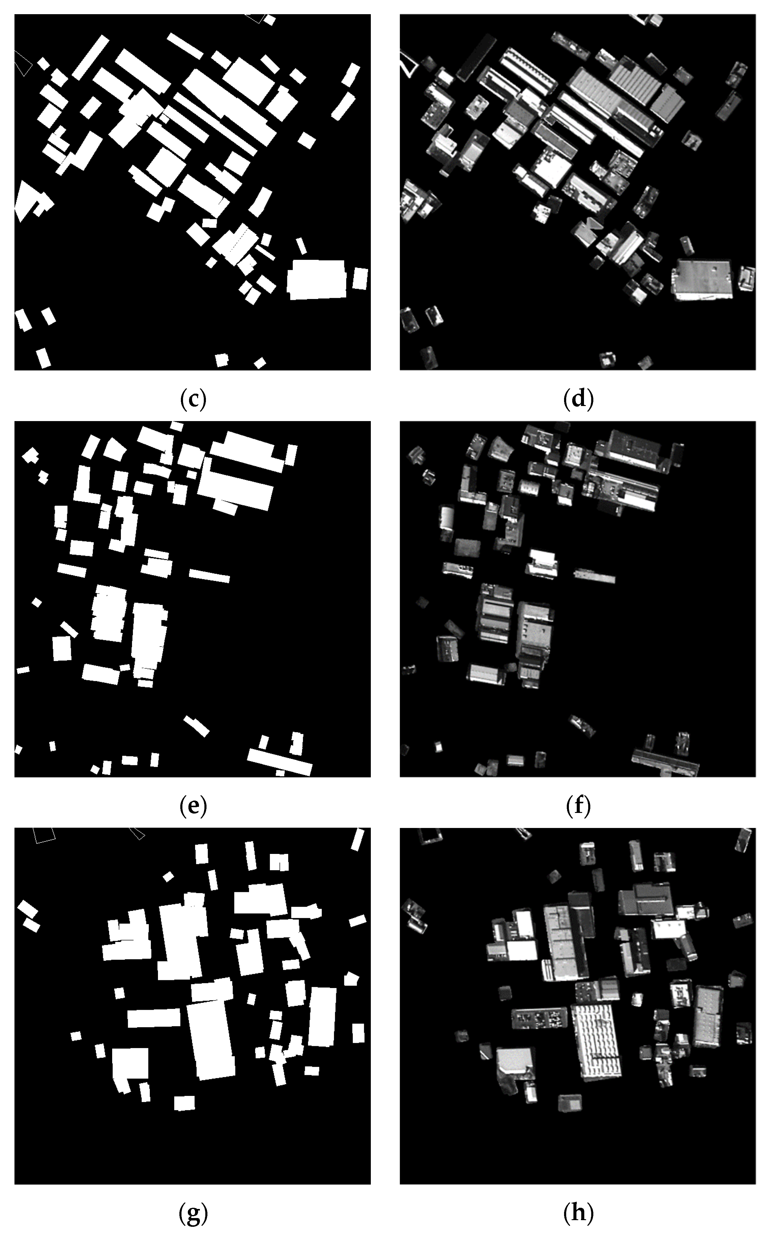
The parameters to be set for building detection based on rectangular approximation are as follows: the detected line segment length screening range is set to [20, 400], the angle range of the two line segments considered to form a right-angle is [80°, 100°], and the maximum distance between endpoints is 15. The experimental results are shown in Figure 6.
Comparing the mask map with the ground truth map reveals that although most of the targets can be detected, there are some false detections in the mask map due to the fact that the selected image is the port area and thus both the trestle and the ship at the port may have a similar shape to the building target, that is, a structure composed of right-angle primitives. There is also a phenomenon of missed detection. For this reason, other features of the target are added to improve the detection accuracy and recall.

3.2. Results of the Diffusion-Based Saliency Model

The compactness-based, local contrast-based, and boundary prior-based saliency maps are fused, and the weights of the three saliency maps are assigned to obtain the saliency map fusion result. For overcoming the complex environment around the building, a bounding box proposal is introduced to optimize the saliency map detection results.
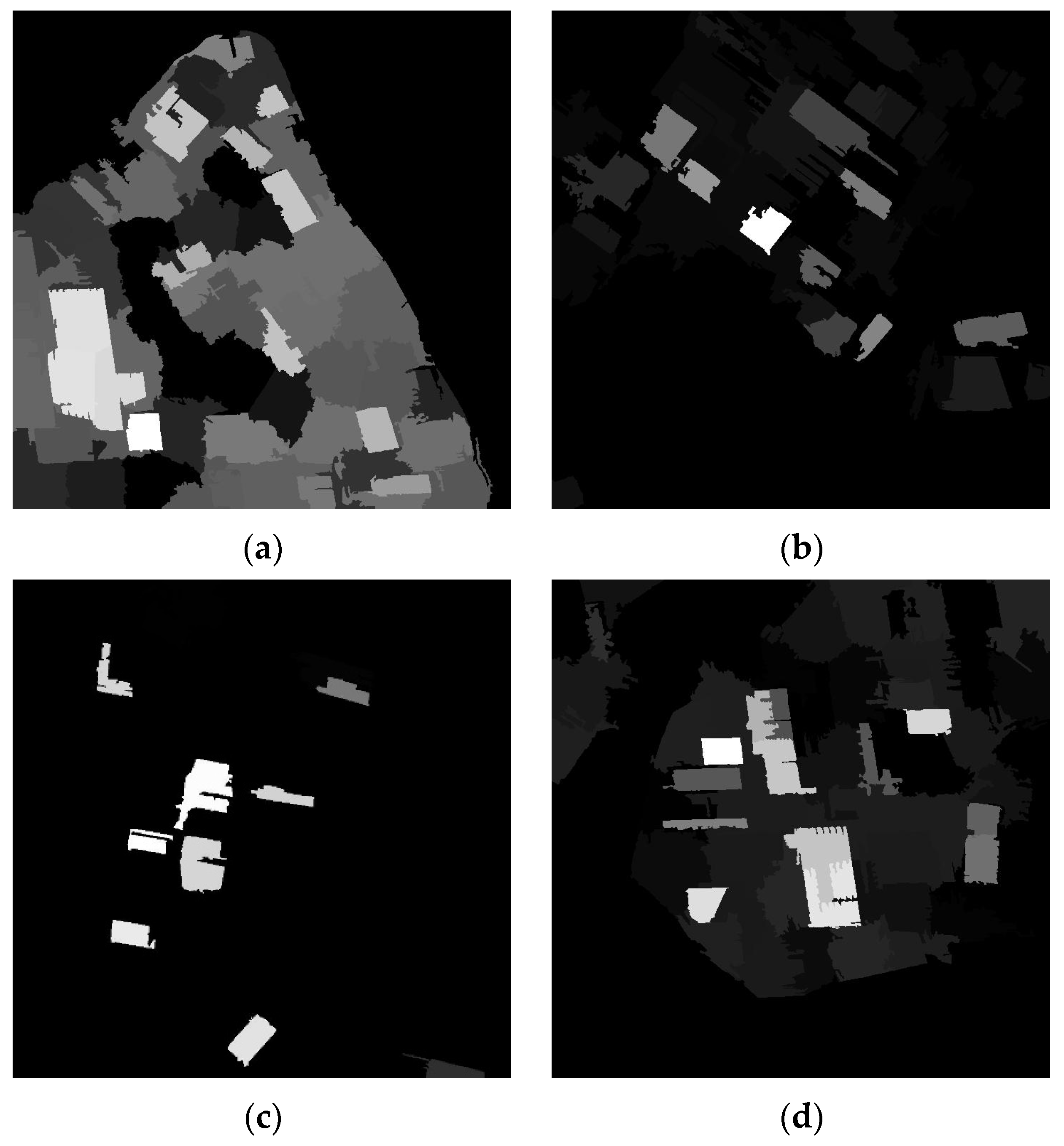
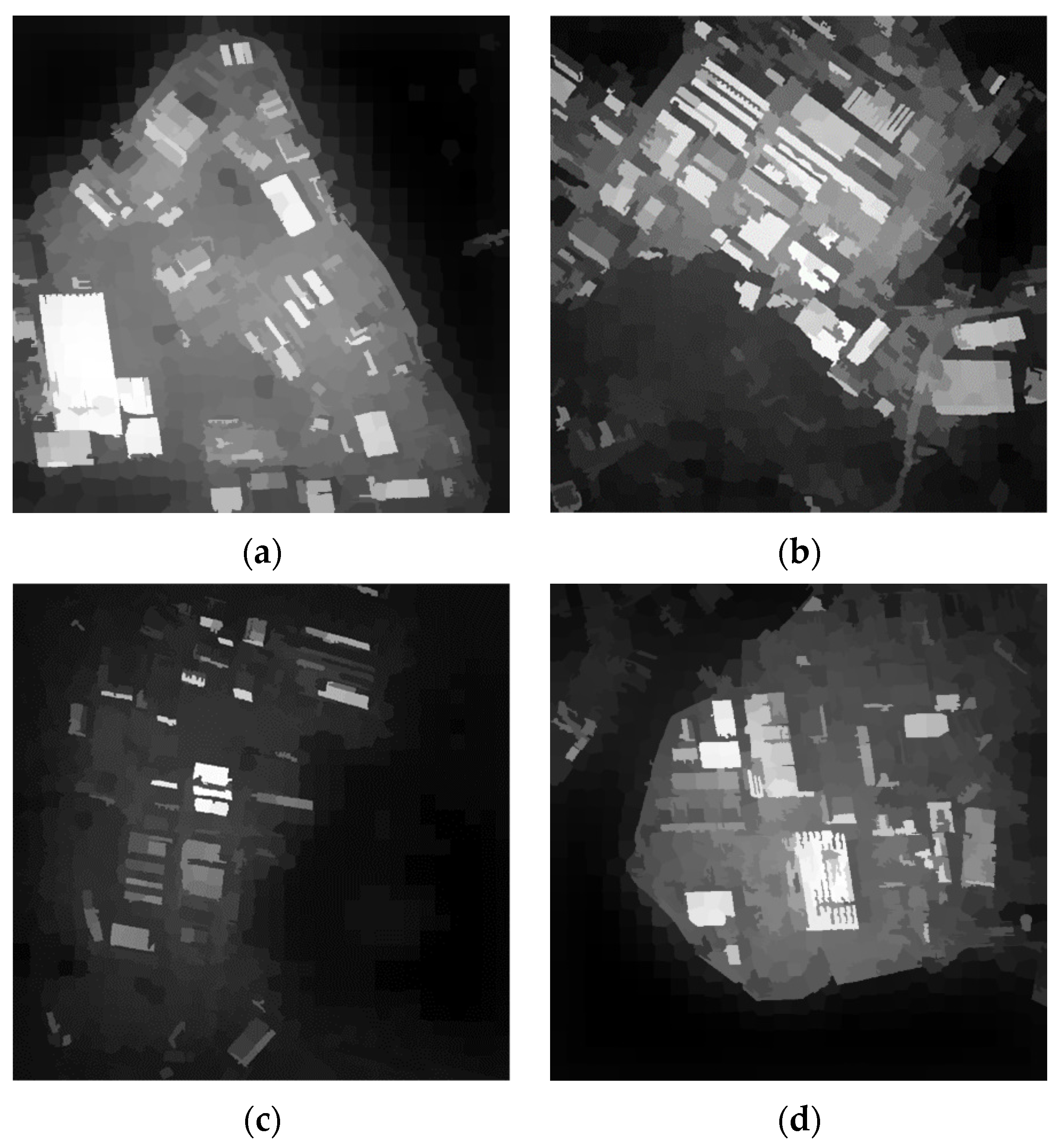
The prospect compactness saliency maps are shown in Figure 7. The local contrast saliency maps are shown in Figure 8. The improved boundary priori saliency maps are shown in Figure 9. The saliency maps after fusion are shown in Figure 10. The foreground mask maps are shown in Figure 11.
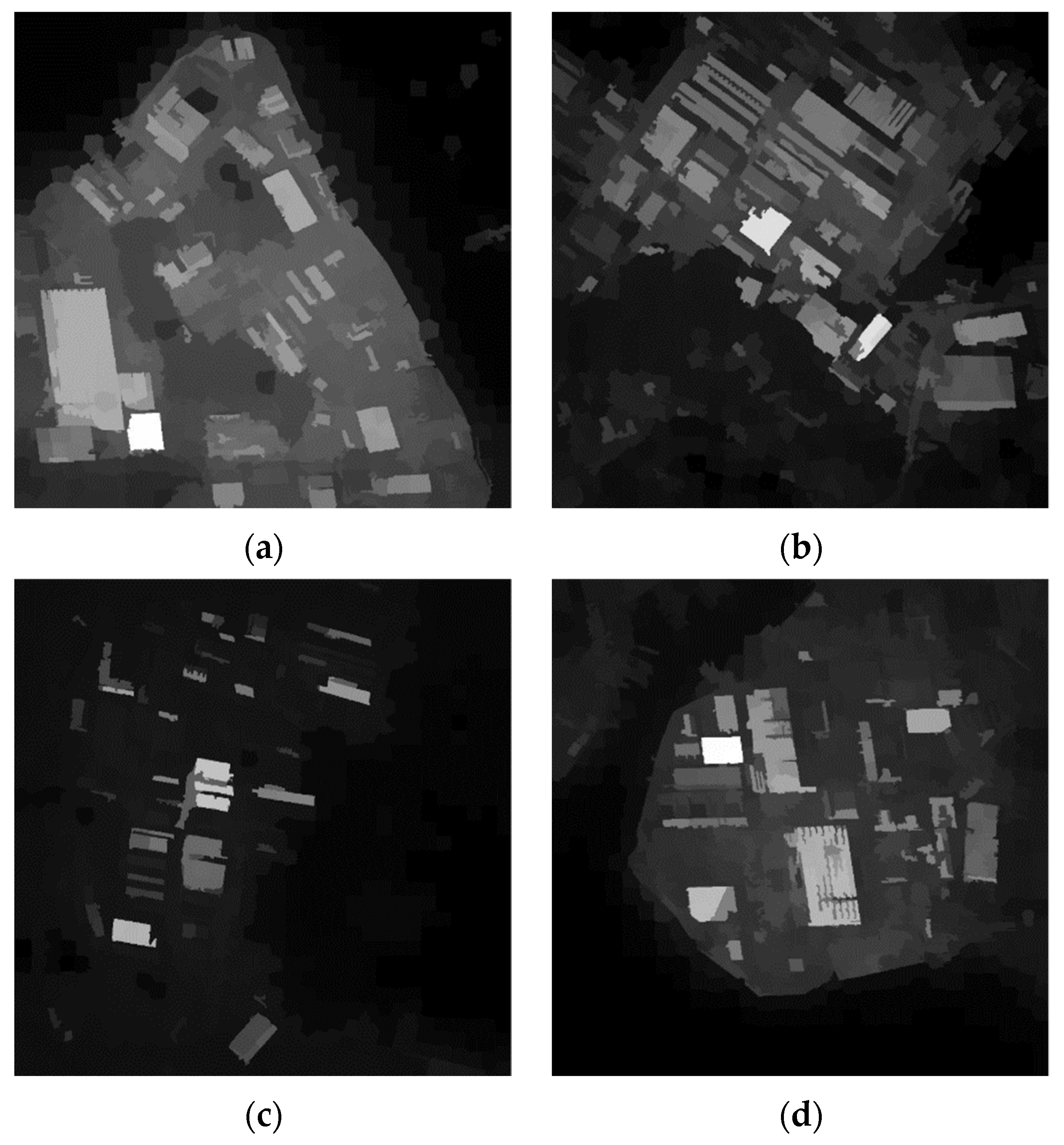
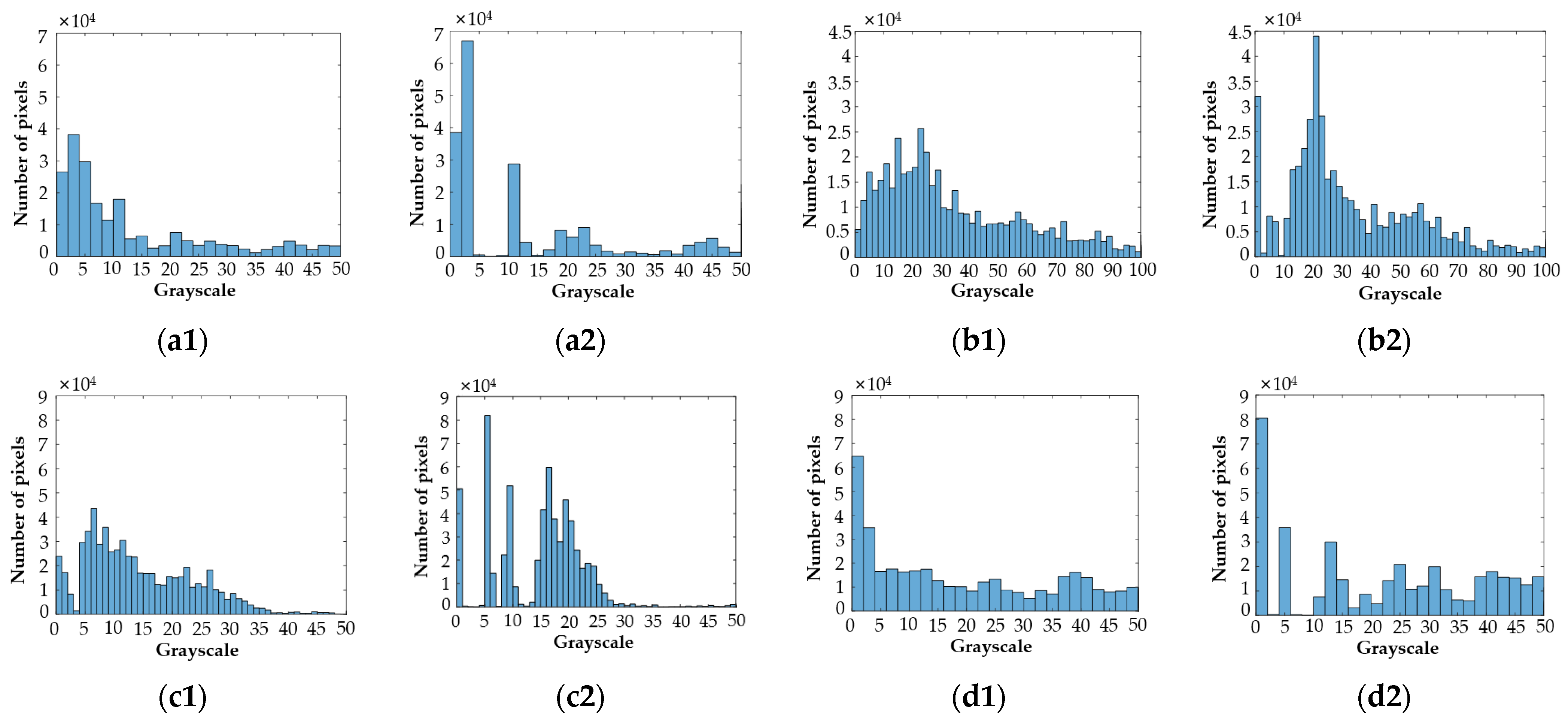
The saliency maps obtained by combining the bounding box proposal are shown in Figure 12. To observe the improvement of the saliency map more visually, the change of the histogram before and after obtaining the foreground mask map is shown in Figure 13. It can be seen that the interference in the environmental background except for the building target is suppressed to some extent. By combining the information from the initial saliency map and the object map, the final saliency map has better results in highlighting objects and suppressing background noise.
The experimental parameters of this paper are designed as follows:
(1)
The number of super-pixel nodes N used in the SLIC model: The SLIC model abstracts the input image into uniform and compact regions. If N is too small, different objects will be mapped to the same super-pixel, which will lead to a decrease in the accuracy of saliency object detection. If N is too large, saliency objects will be mapped to different super-pixels, which may incorrectly suppress saliency regions. The parameter N = 100 is set in the experiment based on compactness and local contrast saliency detection method. The improved saliency detection method with manifold ranking and boundary prior sets the parameter N = W H / 600 , where W and H are the width and height of the experimental image;
(2)
σ for controlling the decay rate of the exponential function: The highest accuracy was achieved when σ 2 = 0.1 in the experiment;
(3)
The equilibrium parameters of the manifold ranking algorithm: The parameters of the literature “Ranking on Data Manifolds” [17] are set with α = 0.99 and μ 2 = 0.5 ;
(4)
After experimental verification, the fusion parameters are chosen as follows: ε c o m = 0.3 , ε l o c = 0.2 , ε o b j = 0.5 for the best detection of the saliency map.
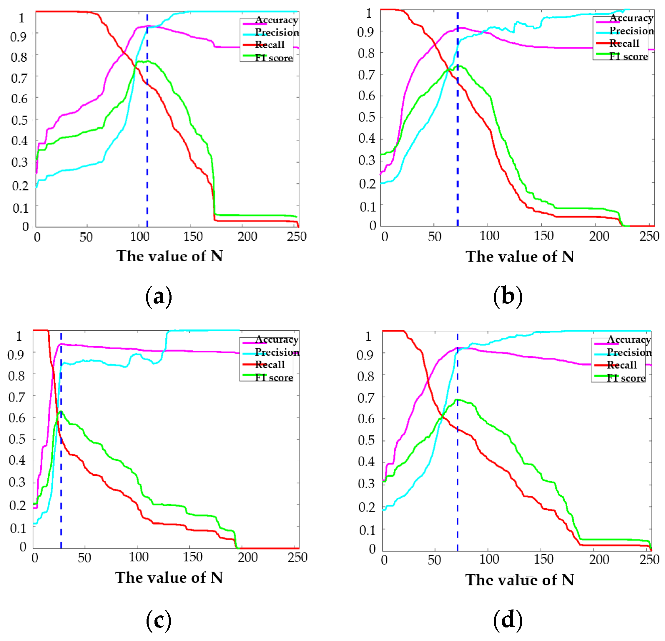
After obtaining the saliency map, the threshold value T f [ 0 , 255 ] of the saliency map is changed from 0 to 255 in order to obtain a better detection effect, and the value of the evaluation index corresponding to the threshold value is calculated by comparing the binary mask map and the binary ground truth map obtained by setting different thresholds of the saliency map, and the change curve of the evaluation indicator is shown in Figure 14.
Figure 9 shows the curves of accuracy, precision, recall and F1 score of the mask map calculated from the saliency map compared with the ground truth map for the case of the threshold value T f [ 0 , 255 ] . The blue line marked in the figure is the threshold position with the highest F1 score, and the adaptive threshold T a is defined as Equation (28).
T a = 2 W H i = 1 W i = 1 H S ( i , j ) 10 ,
where W and H are the width and height of the saliency map S . The saliency map is thresholded with T a to obtain a mask map for building target detection, which is used for the next step of image fusion.

3.3. Fusion and Analysis of Detection Results

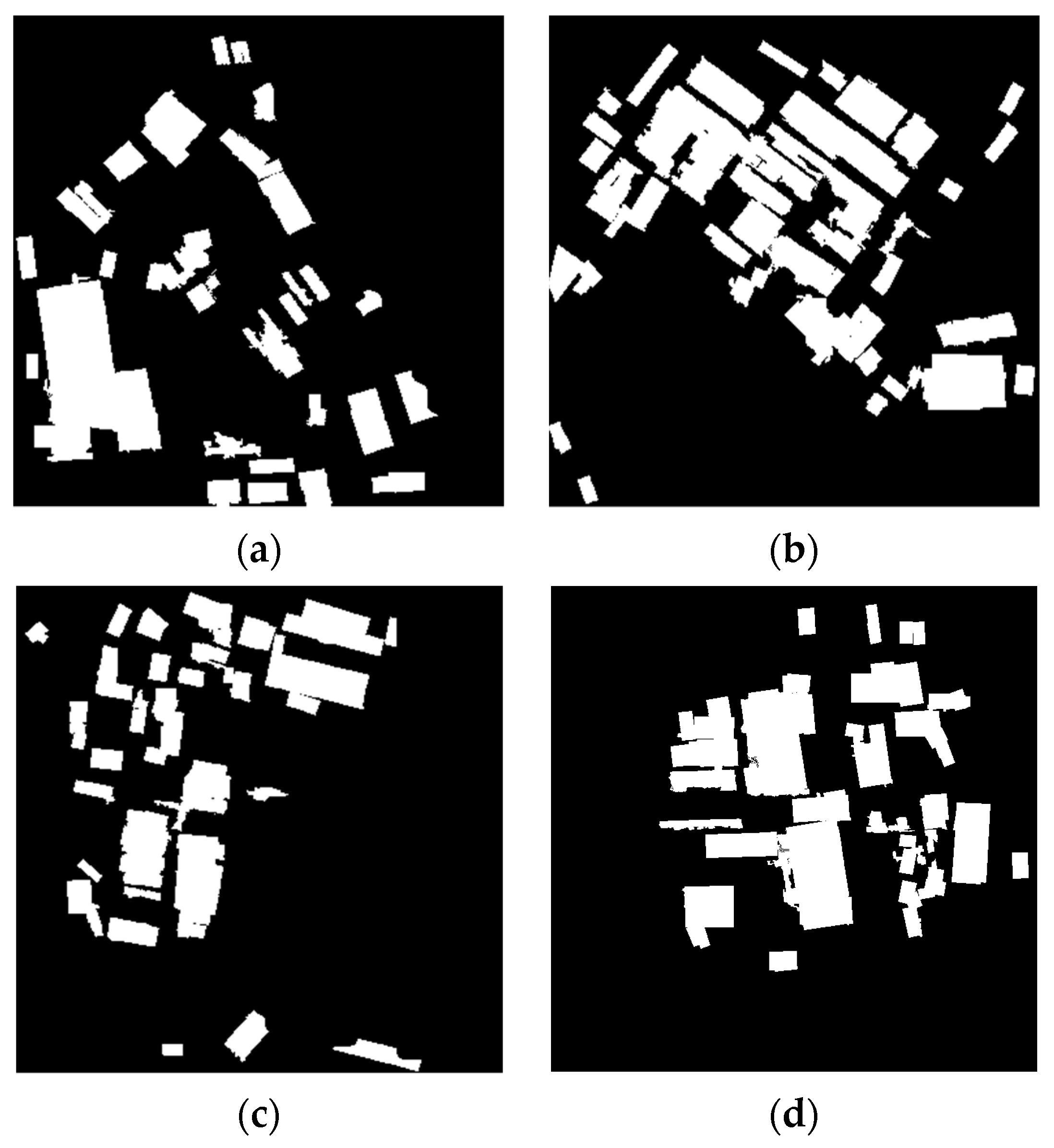
Eliminating the scattered small area interference points, the final obtained building target detection results are shown in Figure 15.
As can be seen from Figure 15, after separating the ocean area, the interference brought by various types of ships and trestles was significantly reduced, and the accuracy of building target detection was improved.
The accuracy, precision, recall, and F1 of the rectangular approximation-based detection results, saliency-based detection results, two mask fusions, and detection results after interference removal were calculated for images I, II, III, and IV, as shown in Table 3, Table 4, Table 5 and Table 6.
From the statistics of the evaluation indicators of the above detection results, it can be seen that the proposed building target detection method, which combines rectangular approximation-based and saliency-based detection results, is able to improve in accuracy, recall, and F1 compared to the detection results of buildings with a single feature. Simultaneously, the overall evaluation index is further improved by removing the ocean area, eliminating the possibility of ships and trestles that cause interference being detected.

4. Discussion

From the experimental results, it can be seen that typical straight line segment detection methods include Hough line detection, LSD and radon transform. Among them, the detection results of the better performing LSD have broken line segments, which is unfavorable to the extraction of right-angle primitives of buildings. Therefore, the constructed broken straight line segment criterion is used to effectively recover the line segments in the image by connecting the broken line segments with parallelism, covariance and broken distance criterion. The detection method of right-angle primitives has ambiguity to tolerate the case of non-adjacent perpendicular straight line segments, and we establish a voting space V R M × N × A of position angles for the extraction of potential right-angle primitives, which obtains the building area and constrains the contour boundary of the building.
The compactness-based, local contrast-based, and boundary prior-based saliency maps are fused, and the weights of the three saliency maps are assigned to obtain the saliency map fusion result. For overcoming the complex environment around the building, a bounding box proposal is introduced to optimize the saliency map detection results. Finally, the detection method based on rectangular approximation and the saliency detection method are combined to further improve the detection of buildings.
The proposed method preserves the contour boundary of the building well, and is an effective method for building detection. Among the existing building target detection methods, deep learning-based building detection methods are more widely used, and we find that many studies are based on pixels to classify buildings. The pixel-based classification and recognition methods can hardly consider the neighborhood information around the pixels, so the contours of buildings cannot be well guaranteed [23].
The existing wavelet transform-based building detection methods, which use different data sources for research, use the binary wavelet transform to detect building edges, which is difficult for the detection of complex building backgrounds and the study of complex building roofs [24,25,26]. Therefore, enhancing building detection constraints can be effective for building extraction, and ensuring the geometric contour of the building while guaranteeing the accuracy of building extraction is the next focus of our research.

5. Conclusions

In this study, building detection in remote sensing image applications was studied. To make the detection of building targets in remote sensing images more accurate, a novel building detection method was developed by fusing the results of the rectangular approximation-based and saliency-based methods to avoid leakage and false detection using individual features. First, for the geometric structure of the top surface of the building target is mostly right-angle primitives composed of mutually perpendicular line segments, this paper proposed a building detection method based on rectangular-approximation and region growth and obtained the saliency map of the building area using a saliency detection model based on the foreground compactness and local contrast of the manifold ranking algorithm. Then, the boundary priori saliency detection method based on the improved manifold ranking algorithm was adopted to successfully detect building targets with low contrast with the background, and the saliency detection results were integrated. Next, introduce the bounding box proposal to remove the environmental noise to obtain the final saliency map, and set the adaptive threshold to obtain the mask map. Finally, the detection results based on rectangular approximation and saliency map were combined and the ocean area in the image was segmented to remove the interference of ships and trestles to achieve the detection of building targets.
In summary, the building target detection method using the fusion of rectangular approximation and saliency detection can avoid the problems of false detection and missing the detection of building targets caused by the fewer gray levels and low resolution of remote sensing images, low contrast between targets and background, shadow occlusion, uneven illumination, and improve the accuracy of building target detection compared with the building target detection method using a single image feature.

Author Contributions

Conceptualization, methodology, visualization, and writing—original draft preparation, Y.M.; data curation, formal analysis, supervision, project administration, funding acquisition, and writing—review and editing, H.C.; investigation, software, resources, and validation, S.Y. All authors have read and agreed to the published version of the manuscript.

Funding

This research was funded by National Natural Science Foundation of China, grant number 61771170.

Institutional Review Board Statement

Not applicable.

Informed Consent Statement

Not applicable.

Data Availability Statement

Not applicable.

Conflicts of Interest

The authors declare no conflict of interest.

Appendix A

Table A1 lists all the acronyms used in this paper.
Table A1. All the acronyms used in this paper.
AbbreviationFull Name
SIFTScale Invariant Feature Transform
VHRVery High Spatial Resolution
CNNConvolutional Neural Network
SVMSupport Vector Machine
LSDLine Segment Detector
SLICSimple Linear Iterative Clustering
TPTrue Positive
FPFalse Positive
FNFalse Negative

References

  1. Ghanea, M.; Moallem, P.; Momeni, M. Building extraction from high-resolution satellite images in urban areas: Recent methods and strategies against significant challenges. Int. J. Remote Sens. 2016, 37, 5234–5248. [Google Scholar] [CrossRef]
  2. Grinias, I.; Panagiotakis, C.; Tziritas, G. MRF-based segmentation and unsupervised classification for building and road detection in peri-urban areas of high-resolution satellite images. ISPRS J. Photogramm. Remote Sens. 2016, 122, 145–166. [Google Scholar] [CrossRef]
  3. Chen, R.; Li, X.; Li, J. Object-based features for house detection from RGB high-resolution images. Remote Sens. 2018, 10, 451. [Google Scholar] [CrossRef] [Green Version]
  4. Hui, J.; Du, M.; Ye, X.; Qin, Q.; Sui, J. Effective building extraction from high-resolution remote sensing images with multitask driven deep neural network. IEEE Geosci. Remote Sens. Lett. 2018, 16, 786–790. [Google Scholar] [CrossRef]
  5. Jing, W.; Xu, Z.; Ying, L. Texture-based segmentation for extracting image shape features. In Proceedings of the 2013 19th International Conference on Automation and Computing (ICAC), London, UK, 13–14 September 2013. [Google Scholar]
  6. Liu, Z.; Li, H.; Zhou, W.; Rui, T.; Tian, Q. Making residual vector distribution uniform for distinctive image representation. IEEE Trans. Circuits Syst. Video Technol. 2016, 26, 375–384. [Google Scholar] [CrossRef]
  7. Mi, W.; Yuan, S.; Pan, J. Building detection in high resolution satellite urban image using segmentation corner detection combined with adaptive windowed hough transform. In Proceedings of the 2013 IEEE International Symposium on Geoscience and Remote Sensing (IGARSS), Melbourne, Australia, 21–26 July 2013; pp. 508–511. [Google Scholar]
  8. Zhang, L.; Zhong, B.; Yang, A. Building change detection using object-oriented LBP feature map in very high spatial resolution imagery. In Proceedings of the 10th International Workshop on the Analysis of Multitemporal Remote Sensing Images (MultiTemp), Shanghai, China, 1 August 2019; pp. 1–4. [Google Scholar]
  9. Vakalopoulou, M.; Karantzalos, K.; Komodakis, N.; Paragios, N. Building detection in very high resolution multispectral data with deep learning features. In Proceedings of the 2015 IEEE International Geoscience and Remote Sensing Symposium (IGARSS), Milan, Italy, 26–31 July 2015; pp. 1873–1876. [Google Scholar]
  10. Zhang, Q.; Wang, Y.; Liu, Q.; Liu, X.; Wang, W. CNN based suburban building detection using monocular high resolution Google Earth images. In Proceedings of the 2016 IEEE International Geoscience and Remote Sensing Symposium (IGARSS), Beijing, China, 10–15 July 2016; pp. 661–664. [Google Scholar]
  11. Liu, Y.; Zhang, Z.; Zhong, R.; Chen, D.; Ke, Y.; Peethambaran, J.; Chen, C.; Sun, L. Multilevel building detection framework in remote sensing images based on convolutional neural networks. IEEE J. Sel. Top. Appl. Earth Obs. Remote Sens. 2018, 11, 3688–3700. [Google Scholar] [CrossRef]
  12. Sidike, P.; Prince, D.; Essa, A. Automatic building change detection through adaptive local textural features and sequential background removal. In Proceedings of the 2016 IEEE International Geoscience and Remote Sensing Symposium (IGARSS), Beijing, China, 10–15 July 2016; pp. 2857–2860. [Google Scholar]
  13. Manandhar, P.; Aung, Z.; Marpu, P.R. Segmentation based building detection in high resolution satellite images. In Proceedings of the 2017 IEEE International Geoscience and Remote Sensing Symposium (IGARSS), Fort Worth, TX, USA, 23–28 July 2017; pp. 3783–3786. [Google Scholar]
  14. Von Gioi, R.G.; Jakubowicz, J.; Morel, J.-M.; Randall, G. LSD: A line segment detector. Image Process. Line 2012, 2, 35–55. [Google Scholar] [CrossRef] [Green Version]
  15. Cong, R.; Lei, J.; Zhang, C.; Huang, Q.; Cao, X.; Hou, C. Saliency detection for stereoscopic images based on depth confidence analysis and multiple cues fusion. IEEE Signal Process. Lett. 2016, 23, 819–824. [Google Scholar] [CrossRef] [Green Version]
  16. Jian, M.; Qi, Q.; Dong, J.; Yin, Y.; Lam, K.M. Integrating QDWD with pattern distinctness and local contrast for underwater saliency detection. J. Vis. Commun. Image Represent. 2018, 53, 31–41. [Google Scholar] [CrossRef]
  17. Yang, C.; Zhang, L.; Lu, H.; Ruan, X.; Yang, M.H. Saliency Detection via Graph-Based Manifold Ranking. Available online: https://openaccess.thecvf.com/content_cvpr_2013/papers/Yang_Saliency_Detection_via_2013_CVPR_paper.pdf (accessed on 14 October 2021).
  18. Zitnick, C.L.; Dollár, P. Edge boxes: Locating object proposals from edges. In Proceedings of the European Conference on Computer Vision, Zurich, Switzerland, 6–12 September 2014; pp. 391–405. [Google Scholar]
  19. Huang, F.; Qi, J.; Lu, H.; Zhang, L.; Ruan, X. Salient object detection via multiple in-stance learning. IEEE Trans. Image Process. 2017, 26, 1911–1922. [Google Scholar] [CrossRef] [PubMed]
  20. Wu, X.; Ma, X.; Zhang, J.; Wang, A.; Jin, Z. Salient object detection via deformed smoothness constraint. In Proceedings of the 2018 25th IEEE International Conference on Image Processing (ICIP), Athens, Greece, 7–10 October 2018; pp. 2815–2819. [Google Scholar]
  21. Otsu, N. A threshold selection method from gray-level histograms. Automatica 1975, 11, 23–27. [Google Scholar] [CrossRef] [Green Version]
  22. Yang, S.; Gu, L.; Li, X.; Jiang, T.; Ren, R. Crop classification method based on optimal feature selection and hybrid CNN-RF networks for multi-temporal remote sensing imagery. Remote Sens. 2020, 12, 3119. [Google Scholar] [CrossRef]
  23. Wang, Y.; Gu, L.; Li, X.; Ren, R. Building extraction in multitemporal high-resolution remote sensing imagery using a multifeature LSTM network. IEEE Geosci. Remote Sens. Lett. 2020, 18, 1645–1649. [Google Scholar] [CrossRef]
  24. Ghaderpour, E.; Pagiatakis, S.; Hassan, Q. A survey on change detection and time series analysis with applications. Appl. Sci. 2021, 11, 6141. [Google Scholar] [CrossRef]
  25. Wang, H.; Li, S.; Zhou, Y.; Chen, S. SAR automatic target recognition using a Roto-translational invariant wavelet-scattering convolution network. Remote Sens. 2018, 10, 501. [Google Scholar] [CrossRef] [Green Version]
  26. Aamir, M.; Pu, Y.-F.; Rahman, Z.; Tahir, M.; Naeem, H.; Dai, Q. A framework for automatic building detection from low-contrast satellite images. Symmetry 2018, 11, 3. [Google Scholar] [CrossRef] [Green Version]
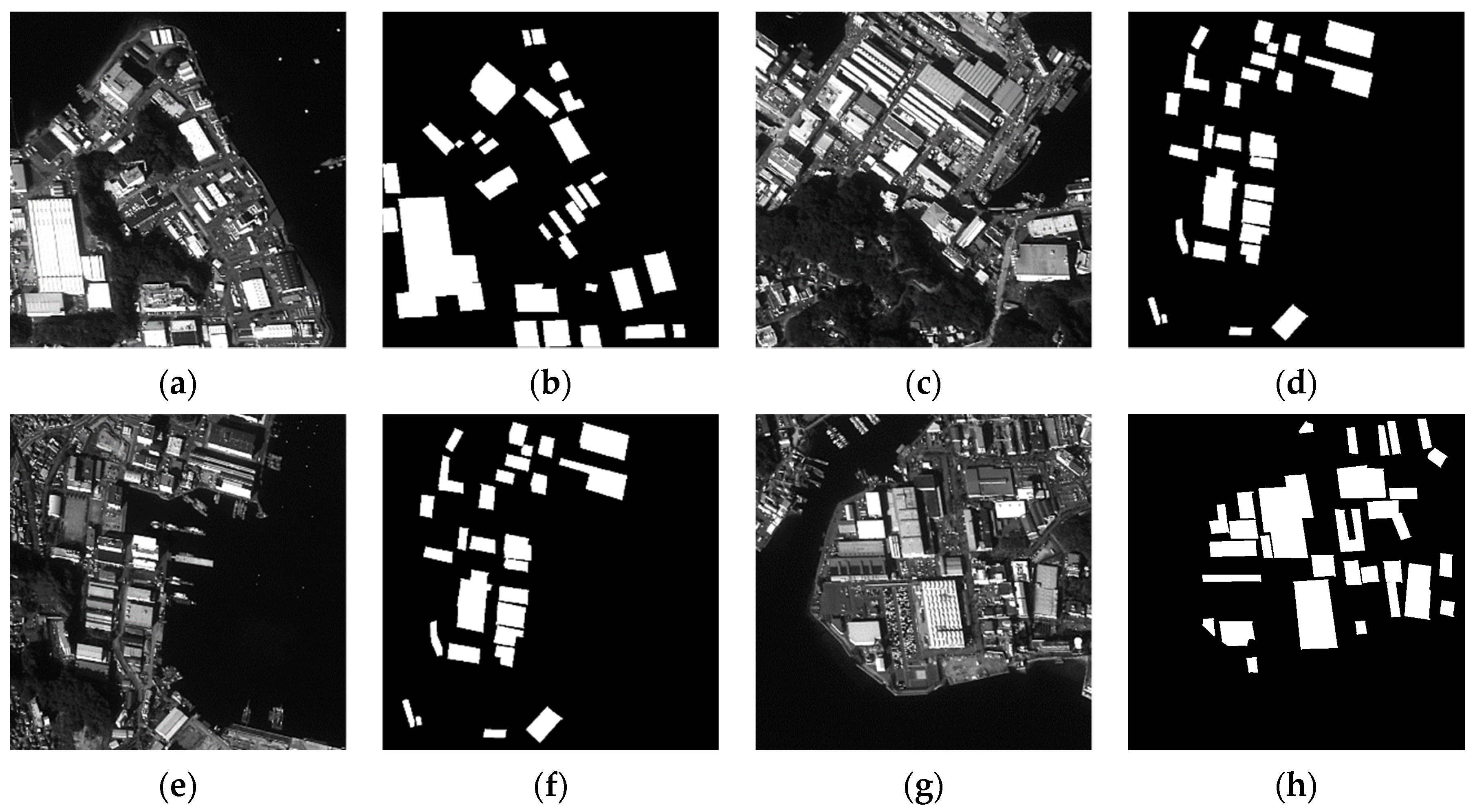
Figure 1. The original experimental images and the corresponding ground truth maps. (a) Original image I, (b) Ground truth I, (c) Original image II, (d) Ground truth II, (e) Original image III, (f) Ground truth III, (g) Original image IV, (h) Ground truth IV.
Algorithms 14 00300 g001
Figure 2. The flowchart of building detection based on rectangular approximation.
Algorithms 14 00300 g002
Figure 3. Line segment detection results. (a) Image I, (b) Image II.
Algorithms 14 00300 g003
Figure 4. The flowchart of saliency model for building detection.
Algorithms 14 00300 g004
Figure 5. The results of super-pixel segmentation. (a) Image I, (b) Image II.
Algorithms 14 00300 g005
Figure 6. Building detection results based on rectangular approximation. (a) Image I mask map, (b) Image I detection result, (c) Image II mask map, (d) Image II detection result, (e) Image III mask map, (f) Image III detection result, (g) Image IV mask map, (h) Image IV detection result.
Algorithms 14 00300 g006aAlgorithms 14 00300 g006b
Figure 7. Prospect compactness saliency maps. (a) Image I, (b) Image II, (c) Image III, (d) Image IV.
Algorithms 14 00300 g007
Figure 8. Local contrast saliency maps. (a) Image I, (b) Image II, (c) Image III, (d) Image IV.
Algorithms 14 00300 g008
Figure 9. The improved boundary priori saliency maps. (a) Image I, (b) Image II, (c) Image III, (d) Image IV.
Algorithms 14 00300 g009
Figure 10. Saliency maps after fusion. (a) Image I, (b) Image II, (c) Image III, (d) Image IV.
Algorithms 14 00300 g010
Figure 11. Foreground mask maps. (a) Image I, (b) Image II, (c) Image III, (d) Image IV.
Algorithms 14 00300 g011
Figure 12. Foreground mask map overlaid with saliency detection result. (a) Image I, (b) Image II, (c) Image III, (d) Image IV.
Algorithms 14 00300 g012
Figure 13. Grayscale histogram comparison before and after overlaying the foreground mask. (a1) Image I before masking, (a2) Image I after masking, (b1) Image II before masking, (b2) Image II after masking, (c1) Image III before masking, (c2) Image III after masking, (d1) Image IV before masking, (d2) Image IV after masking.
Algorithms 14 00300 g013
Figure 14. Variation of each indicator for threshold T f [ 0 , 255 ] . (a) Image I, (b) Image II, (c) Image III, (d) Image IV.
Algorithms 14 00300 g014
Figure 15. Final obtained building detection results. (a) Image I, (b) Image II, (c) Image III, (d) Image IV.
Algorithms 14 00300 g015
Table 1. Jilin-1 Gaofen 03-1 satellite imagery information.
Data/ResolutionRoll Satellite AnglePitch Satellite AngleYaw Satellite Angle
JL1GF03B01/1m−25.601.292.98
Table 2. Captured experimental image information.
ImagePlace/TimeSizeSpace Occupied
Image I
Image II
Image III
Image IV
Port/10 November 2020700 × 700 (I)
700 × 700 (II)
800 × 800 (III)
700 × 700 (IV)
407 KB (I)
483 KB (II)
509 KB (III)
422 KB (IV)
Table 3. Image I detection results.
AccuracyPrecisionRecallF1
Rectangular approximation-based0.90120.74190.64450.6898
Saliency-based0.93280.92070.66270.7706
Fusion0.92040.74560.80870.7759
Interference removal0.93100.81310.77300.7925
Table 4. Image II detection results.
AccuracyPrecisionRecallF1
Rectangular approximation-based0.86890.64290.65470.6487
Saliency-based0.91340.83170.66630.7398
Fusion0.88420.64450.83360.7270
Interference removal0.89580.68070.82160.7445
Table 5. Image III detection results.
AccuracyPrecisionRecallF1
Rectangular approximation-based0.90940.55150.74220.6329
Saliency-based0.93730.83430.50450.6288
Fusion0.91730.57000.87150.6892
Interference removal0.93100.62770.84730.7212
Table 6. Image IV detection results.
AccuracyPrecisionRecallF1
Rectangular approximation-based0.90800.69700.72890.7126
Saliency-based0.92110.90380.55500.6877
Fusion0.91660.69650.82750.7564
Interference removal0.92570.74300.80180.7712
Publisher’s Note: MDPI stays neutral with regard to jurisdictional claims in published maps and institutional affiliations.