3. Clustering Algorithm
Our algorithm for approximating the diameter of a weighted graph uses, as a crucial building block, a clustering strategy which partitions the graph nodes into subsets, called clusters, of bounded (weighted) radius. The strategy grows the clusters around suitable “seed” nodes, called centers, which are selected progressively in batches throughout the algorithm. The challenge is to perform cluster growth by exploiting parallelism while, at the same time, limiting the weight of the edges involved in each growing step, so to avoid increasing excessively the radius of the clusters, which, in turn, directly influences the quality of the subsequent diameter approximation.
Specifically, we grow clusters in stages, where in each stage a new randomly selected batch of centers is added, and clusters are grown around all centers (old and new ones) for a specified radius, which is a parameter of the clustering algorithm. The probability that a node is selected as center increases as the algorithm progresses. The idea behind such a strategy is to force more clusters to grow in regions of the graph which are either poorly connected or populated by edges of large weight, while keeping both the total number of clusters and the maximum cluster radius under control. Note that we cannot afford to grow a cluster boldly by adding all nodes connected to its frontier at once, since some of these additions may entail heavy edges, thus resulting in an increase of the weighted cluster radius which could be too large for our purposes. To tackle this challenge, we use ideas akin to those employed in the
-stepping parallel SSSP algorithm proposed in [
20].
In what follows, we describe an algorithm that, given a weighted graph and a radius parameter r, computes a k-clustering of G with radius slightly larger than r, and k slightly larger than the minimum number of centers of any clustering of G of radius at most r. For each node the algorithm maintains a four-variable state . Variable is the center of the cluster to which u currently belongs to, and is an upper bound to the distance between u and . Variable is the generation of the cluster to which u belongs to, that is, the iteration at which the cluster centerd at started growing. Finally, variable is a Boolean flag that marks whether node u is stable, that is, if the assignment of node u to the cluster centered at is final. Initially, and are undefined, and is false. A node is said to be uncovered if is undefined, and covered otherwise.
For a given graph
and integer parameter
r, Algorithm
RandCluster, whose pseudocode is given in Algorithm 1, builds the required clustering in
iterations (Unless otherwise specified, throughout the paper all logarithms are taken to the base 2. Also, to avoid cluttering the mathematical derivations with integer-rounding notation, we assume
n to be a power of 2, although the results extend straightforwardly to arbitrary
n). In each iteration, all clusters are grown for an extra weighted radius of
, with new centers also being added at the beginning of the iteration. More specifically, initially all nodes are uncovered. In iteration
i, with
, the algorithm selects each uncovered node as a new cluster center with probability
uniformly at random (line 4), and then grows both old and new clusters using a sequence of
growing steps, defined as follows. In a growing step, for each edge
of weight
(referred to as a
light edge) such that
is defined (line 7), the algorithm checks two conditions: whether
v is not stable and whether assigning
v to the cluster centered at
would result in a radius compatible with the one stipulated for
at the current iteration, calculated using the
generation variable
(line 8). If both checks succeed, and if
, then the state of
v is updated, assigning it to the cluster centered at
, updating the distance, and setting
to the generation of
(line 10). In case two edges
and
trigger a concurrent state update for
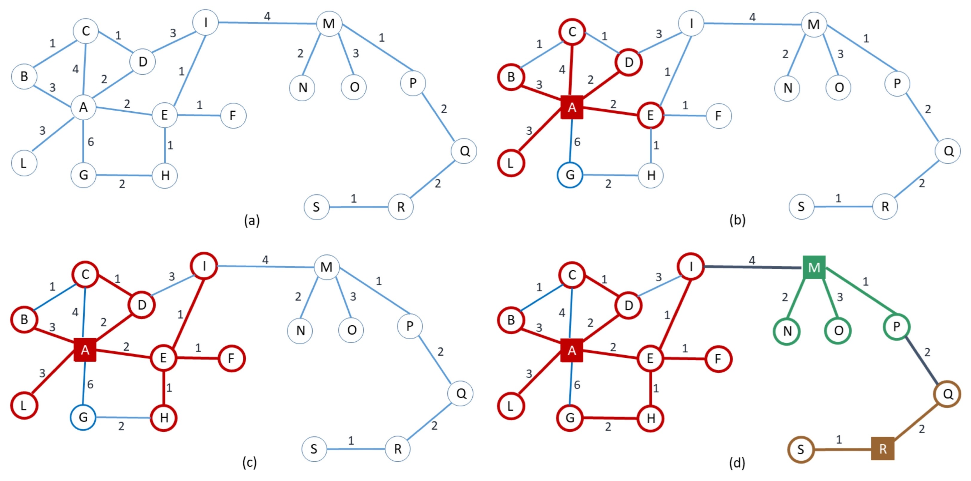
v, we let an arbitrary one succeed. When a growing step does not update any state, then all the covered nodes are marked as stable (line 13) and the algorithm proceeds to the next iteration. An example of one execution of
RandCluster is described pictorially in
Figure 2.
| Algorithm 1:RandCluster |
 |
For a weighted graph and a positive integer x, define as the maximum number of edges in any path in G of total weight at most x. We have:
Theorem 2. Let be a weighted graph, r be a parameter, and let be the minimum integer such that there exists a -clustering of G of radius at most r. Then, with high probability, Algorithm RandCluster performs growing steps and returns an -clustering of G of radius at most .
Proof. The bounds on the number of growing steps and on the radius of the clustering follows straightforwardly from the fact that in each of the iterations of the for loop, the radius of the current (partial) clustering can grow by at most an additive term , hence the growth is attained along paths of distance at most which are covered by traversing at most edges in consecutive growing steps.
We now bound the number of centers selected by the algorithm. We need to consider only the case since, for larger values of , the claimed bound is trivial. The argument is structured as follows. We divide the iterations of the for loop into two groups based on a suitable index h (determined below as a function of and n). The first group comprises iterations with index , where the low selection probability ensures that few nodes are selected as centers. The second group comprises iterations with , where, as we will prove, the number of uncovered nodes decreases geometrically in such a way to counterbalance the increase in the selection probability, so that, again, not too many centers are selected.
Let
and define
h as the smallest integer such that
Since
, we can safely assume that
and define
. For
, we define the event
At the end of iteration of the for loop, at most nodes are still uncovered. We now prove that the event
occurs with high probability. Observe that
where the first equality comes from the definition of conditional probability, and the second is due to the fact that
clearly holds with probability 1.
Consider an arbitrary
, and assume that the event
holds. We prove that, conditioned on this event,
holds with high probability. Let
be the set of nodes already covered at the beginning of iteration
. By hypothesis, we have that
. We distinguish two cases. If
, then
clearly holds with probability 1. Otherwise, it must be
Let
be a
-clustering of
G with radius
r, whose existence is implied by the definition of
, and divide its clusters into two groups: a cluster
is called
small if
, and
large otherwise. Let
be the set of small clusters. We can bound the number of uncovered vertices contained in the small clusters as follows:
It then follows that, overall, the
large clusters contain at least half of the nodes that the algorithm has yet to cover at the beginning of iteration
. We now prove that, with high probability, at least one center will be selected in each large cluster. Consider an arbitrary large cluster
C. By Equations (
1) and (
3), we have that the number of uncovered nodes in
C is at least
Since in iteration
, an uncovered node becomes a center with probability
, the probability that no center is selected from
C is at most
By applying the union bound over all large clusters and taking the complement of the probability, it immediately follows that the probability that each large cluster has at least one center being selected among its uncovered nodes is at least . Now, it is easy to see that in each iteration, in particular, in iteration , all nodes at distance at most from the newly selected centers will be covered by some cluster (either new or old). Consequently, since the radius of any cluster of is , we have that with probability at least , at the end of iteration all nodes in large clusters are covered. Thus, the nodes still uncovered at the of the iteration can belong only to small clusters in , and, from what was observed before, there are at most of them.
By multiplying the probabilities of the conditional events , we conclude that happens with probability at least , where the last bound follows from Bernoulli’s inequality and the fact that .
We can finally bound the number of centers selected during the execution of the algorithm. We do so by partitioning the iterations into three groups based on the iteration index j, and by reasoning on each group as follows:
Iterations j, with : since, at the beginning of each such iteration j, the number of uncovered nodes is clearly and the selection probability for each uncovered node is , by the Chernoff bound we can easily show that centers are selected, with probability at least .
Iterations j, with : by conditioning on the event , we have that at the beginning of each such iteration j the number of uncovered nodes does not exceed and the selection probability for an uncovered node is . Since , by the Chernoff bound we can easily show that in iteration j, centers are selected, with probability at least .
Iteration : by conditioning on the event we have that at the beginning of iteration the number of uncovered nodes is , and since in this iteration the selection probability is 1, all uncovered nodes will be selected as centers.
Putting it all together we have that, by conditioning on
and by Bernoulli’s inequality, with probability at least
the total number of centers selected by the algorithm is
The theorem follows. □
Algorithm RandCluster exhibits the following important property, which will be needed in proving the diameter approximation. Define the light distance between two nodes u and v of G as the weight of the shortest path from u to v consisting only of light edges, that is, edges of weight at most (note that this distance is not necessarily defined for every pair of nodes). We have the following.
Observation 1. For a specific execution of RandCluster, given a center selected at iteration i, and a node at light distance d from c, v cannot be covered by c (i.e., cannot be set to c by the algorithm) in less than iterations. Also, by the end of iteration , v will be covered by some cluster center (possibly c).
Proof. Let be a path of light edges of total weight d between c and v. In each iteration of the algorithm, the cluster centered at c is allowed to grow for a length at most along . Also, an easy induction suffices to show that any node at light distance at most from c on the path will surely be covered (by c or another center) by the end of iteration s. □
An immediate consequence of the above observation is the following. Let be a center selected at iteration i, and a node at light distance d from c. No center selected at an iteration and at distance at least d from v is able to cover v. The reason is that any such center would require the same number of iterations to reach v as c, and by the time it is able to reach v, v would have already been reached by c (or some other center) and marked as stable, which would prevent the reassignment to other centers.
4. Diameter Approximation Strategy
We are now ready to describe our clustering-based strategy to approximate the diameter of a graph G. For any fixed value , we run RandCluster to obtain a clustering . By Theorem 2, we know that, with high probability, has radius and consists of clusters, where is the minimum number of clusters among all the clusterings of G with radius r. Also, we recall that is represented by the tuples , for every , where is the center of the cluster of u, and is an upper bound to .
As in [
16], we define a weighted auxiliary graph
associated with
where the nodes correspond to the cluster centers and, for each edge
of
G with
, there is an edge
in
of weight
. In case of multiple edges between clusters, we retain only the one yielding the minimum weight. (See
Figure 3 for the auxiliary graph associated to the clustering described in
Figure 2).
Let
(resp.,
) be the diameter of
G (resp.,
). We approximate
with
It is easy to see that . The following theorem provides an upper bound to .
Theorem 3. If , then with high probability.
Proof. Since , and, by hypothesis, , it is sufficient to show that . To this purpose, let us fix an arbitrary pair of distinct clusters and a shortest path in G between their centers of (minimum) weight . Let be the (not necessarily simple) path of clusters in traversed by , and observe that, by shortcutting all cycles in , we have that the distance between the nodes associated to the centers of and in is upper bounded by plus twice the sum of the radii of the distinct clusters encountered by . We now show that, with probability at least , this latter sum is . Then the theorem will immediately follow by applying the union bound over all pairs of distinct clusters. We distinguish the following two cases.
Case 1. Suppose that
(hence,
, since we assumed
) and let
be the index of the first iteration where some centers are selected. By applying a standard Chernoff bound ([
31], Corollary 4.6) we can easily show that
centers are selected in Iteration
i, with probability at least
. Moreover, since all nodes in
G are at light distance at most
from the selected centers, we have that, by virtue of Observation 1, all nodes will be covered by the end of Iteration
i. Therefore, with probability at least
,
contains
clusters and it easily follows that its weight is
.
Case 2. Suppose now that . We show that, with high probability, at most clusters intersect (i.e., contain nodes of ). Observe that can be divided into subpaths, where each subpath is either an edge of weight or a segment of weight . We next show that the nodes of each of the latter segments belong to clusters, with high probability. Consider one such segment S. Clearly, all clusters containing nodes of S must have their centers at light distance at most from S (i.e., light distance at most from the closest node of S).
For , let be the set of nodes whose light distance from S is between and , and observe that any cluster intersecting S must be centered at a node belonging to one of the ’s. We claim that, with high probability, for any j, there are clusters centered at nodes of which may intersect S. Fix an index j, with , and let be the first iteration of the for loop of RandCluster in which some center is selected from . By Observation 1, iterations are sufficient for any of these centers to cover the entire segment. On the other hand, any center from needs at least iterations to touch the segment. Hence, we have that no center selected from at Iteration or higher can cover a node of S, since by the time it reaches S, the nodes of the segment are already covered and stable.
We now show that the number of centers being selected from in Iterations and is . For a suitable constant c, we distinguish two cases.
. Then the bound trivially holds.
. Let h be an index such that in Iteration h the center selection probability is such that . Therefore, in Iteration the expected number of centers selected from is . By applying the Chernoff bound, we can prove that, with high probability, the number of centers selected from in Iteration is and that the number of centers selected in any iteration is . Furthermore, observe that, with high probability, : indeed, if no center is selected in iterations up to the , with high probability at least one is chosen at iteration h, since we just proved that are selected in iteration h.
Therefore, we have that the total number of centers selected from
in Iterations
and
(and thus the only centers from
which may cover nodes of
S) is
. Overall, considering all
’s, the nodes of segment
S will belong to
clusters, with high probability. By applying the union bound over all segments of
, we have that
clusters intersect
, with high probability. It is easy to see that by suitably selecting the constants in all of the applications of the Chernoff bound, the high probability can be made at least
. Therefore, with such probability we have:
where last equality follows from the hypothesis
. □
An important remark regarding the above result is in order at this point. While the upper bound on the approximation ratio does not depend on the value of parameter r (as long as ), this value affects the efficiency of the strategy. In broad terms, a larger r yields a clustering with fewer clusters, hence a smaller auxiliary graph whose diameter can be computed efficiently with limited main memory, but requires a larger number of growing steps in the execution of RandCluster, hence a larger number of synchronizations in a distributed execution. In the next section we will show how to make a judicious choice of r which strikes a suitable space-round tradeoff in MapReduce.
5. Implementation in the MapReduce Model
In this section we describe an algorithm for diameter approximation in MapReduce, which uses sublinear local memory and linear aggregate memory and, for an important class of graphs which includes well-known instances, features a round complexity asymptotically smaller than the one required to obtain a 2-approximation through the state-of-the-art SSSP algorithm by [
20]. The algorithm runs the clustering-based strategy presented in the previous section for geometrically increasing guesses of the parameter
r, until a suitable guess is identified which ensures that the computation can be. carried out within a given local memory budget.
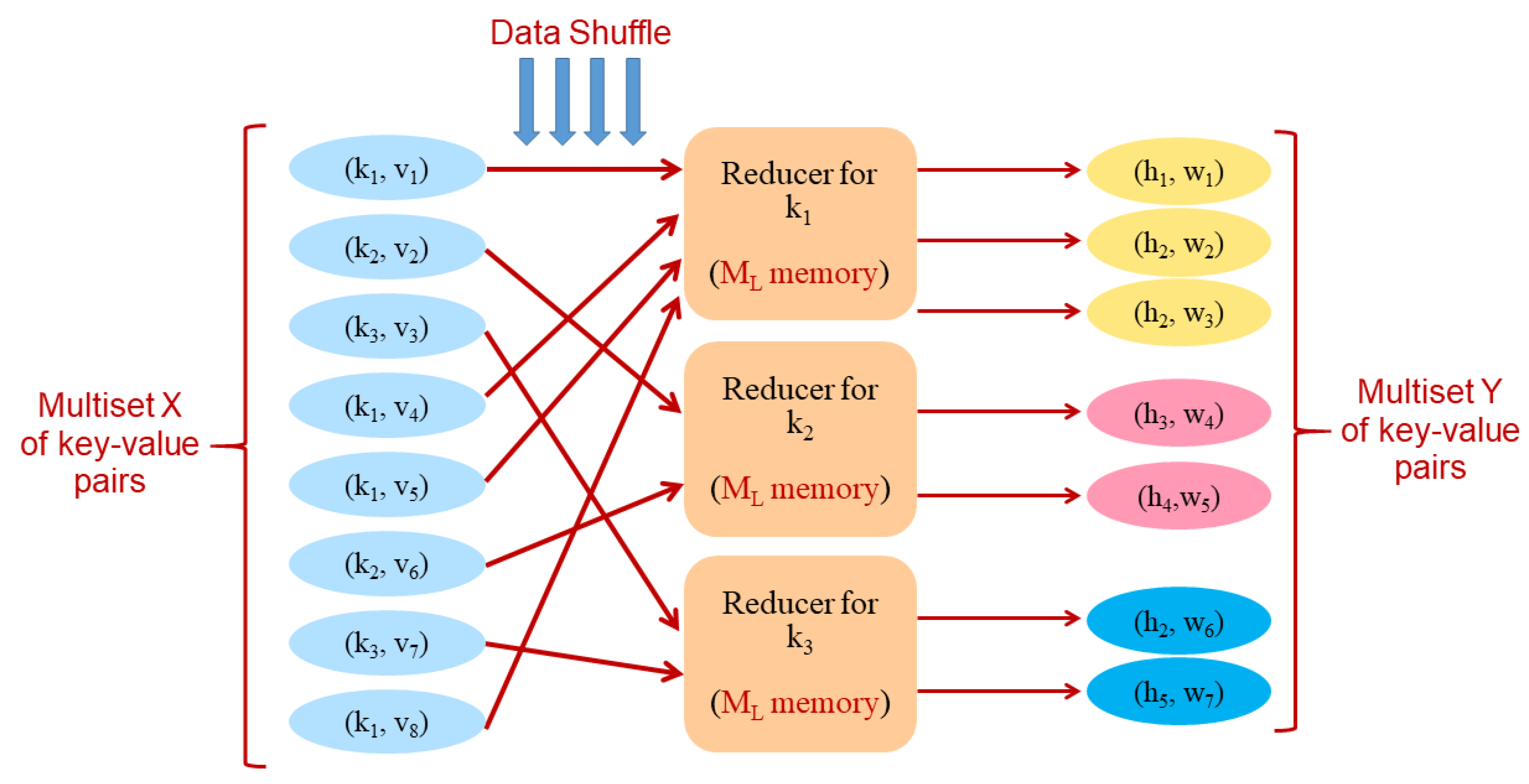
Recall that the diameter-approximation strategy presented in the previous section is based on the use of Algorithm RandCluster to compute a clustering of the graph, and that, in turn, RandCluster entails the execution of sequences of growing steps. A growing step (lines 7–10 of Algorithm 1) can be implemented in MapReduce as follows. We represent each node by the key-value pair and each edge by the two key-value pairs and . We then sort all key-value pairs by key so that for every node u there will be a segment in the sorted sequence starting from and followed by the pairs associated to its incident edges u. At this point, a segmented prefix operation can be used to create, for each edge two pairs and , which are then gathered by a single reducer to perform the possible update of or as specified by lines 8–10 of Algorithm 1. A final prefix operation can be employed to determine the final value of each 4-tuple , by selecting the update with minimum .
By Theorem 1, each sorting and prefix operation can be implemented in MR with rounds and linear aggregate memory. The MapReduce implementation of all other operations specified by Algorithm 1 is simple and can be accomplished within the same memory and round complexity bounds as those required by the growing steps. Recall that for a weighted graph G, we defined to be the maximum number of edges in any path of total weight at most x. By combining the above discussion with the results of Theorems 1 and 2, we have:
Lemma 1. Let G be a connected weighted graph with n nodes and m edges. On the MR model algorithm RandCluster can be implemented inrounds, with . In particular, if , for some constant , the number of rounds becomes . We are now ready to describe in detail our MapReduce algorithm for diameter approximation. Consider an n-node connected weighted graph G, and let be the minimum edge weight. For a fixed parameter , the algorihm runs RandCluster for geometrically increasing values of r, namely , with , until the returned clustering is such that the corresponding auxiliary graph has size (i.e., number of nodes plus number of edges) . At this point, the diameter of is computed using a single reducer, and the value , where is the radius of , is returned as an approximation to the true diameter . We have:
Theorem 4. Let G be connected weighted graph with n nodes, m edges, and weighted diameter . Also, let be an arbitrarily fixed constant and define as the minimum radius of any clustering of G with at most clusters. With high probability, the above algorithm returns an estimate such that , and can be implemented in the MR model using rounds, with and .
Proof. Let be the first radius in the sequence such that . Define (resp., ) as the minimum number of clusters in a clustering of G with radius (resp., ). It is straightforward to see that . Since, by hypothesis, , we have that . By Theorem 2, with high probability RandCluster returns a clustering with clusters whose corresponding auxiliary graph has size . Therefore, with high probability, the MapReduce algorithm will complete the computation of the approximate diameter after an invocation of RandCluster with radius at most .
By Lemma 1, each invocation of
RandCluster can be implemented in MapReduce using
rounds with
and
. In particular, the round complexity of the last invocation (with radius at most
) will upper bound the one of any previous invocation. Considering the fact that
, we have that the round complexity of each invocation is
. Note that
, therefore the maximum number of values
r for which
RandCluster is executed is
. Since
, where
is the maximum edge weight, and
is polynomial in
n, as we assumed at the beginning of
Section 3, we have that the maximum number of invocations of
RandCluster is
. Therefore, the aggregated round complexity of all the invocations of
RandCluster up to the one finding a suitably small clustering is
. Moreover, it is easy to see that the computation of the auxiliary graph after each invocation of
RandCluster and the computation of the diameter after the last invocation, which is performed on an auxiliay graph of size
, does not affect neither the asymptotic round complexity nor the memory requirements.
Finally, the bound on the approximation follows directly from Theorem 3, while the bounds on and derive from Lemma 1 and from the previous discussion. □
We observe that the term
which appears in the round complexity of the algorithm stated in the above theorem, depends on the graph topology. In what follows, we will prove an upper bound to
, hence an upper bound to the round complexity, in terms of the
doubling dimension of
G, a topological notion which was reviewed in
Section 2.2. To this purpose, we first need the following technical lemma.
Lemma 2. Let G be a graph with n nodes and maximum degree d. If we remove each edge independently with probability at least , then, with high probability, the graph becomes disconnected and each connected component has size .
Proof. Let be a graph obtained from by removing each edge in E with probability . Equivalently, each edge in E is included in with probability , independent of other edges. If has a connected component of size k then it must have a tree of size k. We prove the claim by showing that for , the probability that a given vertex v is part of a tree of size is bounded by .
For a fixed vertex
, let
and let
be the set of vertices in
connected to
but not to
,
, i.e.,
Consider a Galton–Watson branching process [
32]
, with
, and
, where
are independent, identically distributed random variables with a Binomial distribution
. Clearly for any
, the distribution of
is stochastically upper bounded by the distribution of
. For a branching process with i.i.d. offspring distributions as the one we are considering, the
total progeny can be bound as follows ([
33], Theorem 3.13) [
34]
where the
are independent random variables with the same distribution as the offspring distribution of the branching process, which in this case is a Binomial with parameters
and
p.
Now, we have
, therefore, by applying a Chernoff bound, the probability that
v is part of a tree of size
is bounded by
If
, with
, then we have
By union bound over the n nodes, the probability that the graph has a connected component of size greater than is bounded by . □
On weighted graphs, the result of Lemma 2 immediately implies the following observation.
Observation 2. Given a graph of maximum degree d with edge weights uniformly distributed in , if we remove the edges whose weight is larger than or equal to , then with high probability the graph becomes disconnected and the size of each connected component is . That is, in any simple path the number of consecutive edges with weight less than is , with high probability.
Observation 2 allows us to derive the following corollary of Theorem 4. Recall that denotes the weighted diameter of G. With , instead, we denote its unweighted diameter.
Corollary 1. Let G be a connected graph with n nodes, m edges, maximum degree , doubling dimension D, and positive edge weights chosen uniformly at random from , with . Also, let be an arbitrarily fixed constant. With high probability, an estimate such that , can be computed in rounds on the MR model with and .
Proof. Given the result of Theorem 4, in order to prove the corollary we only need to show the bound on the number of rounds. From the statement of Theorem 4, recall that, with high probability, the number of rounds is , where is the minimum radius of any clustering of G with at most clusters.
By iterating the definition of doubling dimension starting from a single ball of unweighted radius containing the whole graph, we can decompose G into disjoint clusters of unweighted radius . Since is the maximum edge weight, we have that . We will now give an upper bound on . By Lemma 2 and Observation 2, we have that by removing all edges of weight , with high probability the graph becomes disconnected and each connected component has nodes. As a consequence, with high probability, any simple path in G will traverse an edge of weight every nodes. This implies that a path of weight at most has at most edges, and the corollary follows. □
The above corollary ensures that, for graphs of constant doubling dimension, we can make the number of rounds polynomially smaller than the unweighted diameter
. This makes our algorithm particularly suitable for inputs that are otherwise challenging in MapReduce, like high-diameter, mesh-like sparse topologies (a mesh has doubling dimension 2). On these inputs, performing a number of rounds sublinear in the unweighted diameter is crucial to obtain good performance. In contrast, algorithms for the SSSP problem perform a number of rounds linear in the diameter. Consider for instance
-stepping that, being a state of the art parallel SSSP algorithm, is our most natural competitor. Given a graph
G with random uniform weights, the analysis in [
20] implies that under the linear-space constraint a natural MapReduce implementation of
-stepping requires
rounds. In the next section, we will assess experimentally the difference in performance between our algorithm and
-stepping.
6. Improved Performance for Unweighted Graphs
We can show that running the MapReduce implementation described in the previous section on unweighted graphs is faster than in the general case. In fact, in the unweighted case, the growing step is very efficient, since once a node is covered for the first time, it is always with the minimum distance from its center, so it will not be further updated. (In fact, in the unweighted case the growing step is conceptually equivalent to one step of a BFS-like expansion). This results in an improvement in the round complexity by a doubly logarithmic factor, as stated in the following corollary to Theorem 4.
Corollary 2. Let G be a connected unweighted graph with n nodes, m edges, and doubling dimension D. Also, let be an arbitrarily fixed constant. With high probability, an estimate such that can be computed in rounds on the MR model with and .
Proof. The approximation bound is as stated in Theorem 4. For what concerns the round complexity, we first observe that an unweighted graph can be regarded as a weighted graph with unit weights. On such a graph, we have , for every positive integer x. Thus, by Lemma 1, each execution of RandCluster can be implemented in rounds in the MR model with and . From the statement of Theorem 4, recall that is the minimum radius of any clustering of G with at most clusters. As argued in the proof of that theorem, the round complexity of the algorithm is dominated by the executions of RandCluster, which are performed for geometrically increasing values of r up to a value at most , thus yielding an overall round complexity of .
By reasoning as in the proof of Corollary 1 we can show that G can be decomposed into disjoint of radius , which thus provides an upper bound to . The corollary follows. □
In the case of unweighted graphs, the most natural competitor for approximating the diameter is a simple BFS, instead of
-stepping. However, the same considerations made at the end of the previous section apply, since any natural MapReduce implementation of BFS also requires
rounds, similarly to
-stepping. Another family of competitors is represented by neighbourhood function-based algorithms [
10,
12,
15], which we reviewed in
Section 1.1. These algorithms, like the BFS, require
rounds, and are therefore outperformed by our approach on graphs with constant doubling dimension.
As a final remark on our theoretical results for both the weighted and the unweighted cases, we observe that the
bound on the ratio between the diameter returned by our strategy and the exact diameter may appear rather weak. However, these theoretical bounds are the result of a number of worst-case approximations which, we conjecture, are unlikely to occur in practice. In fact, in the experiments reported in
Section 7.1, our strategy exhibited an accuracy very close to the one of the 2-approximation based on
-stepping. Although to a lesser extent, the theoretical bounds on the round complexities of the MapReduce implementation may suffer from a similar slackness. An interesting open problem is to perform a tighter analysis of our strategy, at least for specific classes of graphs.
7. Experiments
We implemented our algorithms with Rust 1.41.0 (based on LLVM 9.0) on top of Timely Dataflow (
https://github.com/TimelyDataflow/timelydataflow) (compiled in
release mode, with all available optimizations activated). Our implementation, which is publicly available (
https://github.com/Cecca/diameter-flow/), has been run on a cluster of 12 nodes, each equipped with a 4 core I7-950 processor clocked at a maximum frequency of
GHz and 18 GB RAM, connected by a 10 Gbit Ethernet network. We configured Timely Dataflow to use 4 threads per machine.
We implemented the diameter-approximation algorithm as described in
Section 5 (referred to as
ClusterDiameter in what follows), by running several instances of
RandCluster, each parametrized by a different value of
r, until a clustering is found whose corresponding auxiliary graph fits into the memory of a single machine. In order to speed up the computation of the diameter of the auxiliary graph, rather than executing the classical exact algorithm based on all-pairs shortest paths, we run two instances of Dijkstra’s algorithm: the first from an arbitrary node, the second from the farthest reachable node, reporting the largest distance found in the process. We verified that this procedure, albeit providing only a 2-approximation in theory, always finds a very close approximation to the diameter in practice, in line with the findings of [
6], while being much faster than the exact diameter computation. The only other deviation from the theoretical algorithm concerns the initial value of
r, which is set to the average edge weight (rather than
) in order to save on the number of guesses.
We compared the performance of our algorithm against the 2-approximation algorithm based on
-stepping [
20], which we implemented in the same Rust/Timely Dataflow framework. In what follows, we will refer to this implementation as
DeltaStepping. For this algorithm, we tested several values of
, including fractions and multiples of the average edge weight, reporting, in each experiment, the best result obtained over all tested values of
.
We experimented on three graphs: a web graph (
sk-2005), a social network (
twitter-2010), (both downloaded from the WebGraph collection [
35,
36]:
http://law.di.unimi.it/datasets.php) and a road network (
USA, downloaded from
http://users.diag.uniroma1.it/challenge9/download.shtml). Since both
sk-2005 and
twitter-2010 are originally unweighted graphs, we generated a weighted version of these graphs by assigning to each edge a random integer weight between 1 and
n, with
n being the number of nodes. Also, since the road network
USA, on the other hand, is small enough to fit in the memory of a single machine, we inflated it by generating the cartesian product of the network with a linear array of
S nodes and unit edge weights, for a suitable scale parameter
S. In the reported experiments we used
. The rationale behind the use of the cartesian product was to generate a larger network with a topology similar to the original one. For each dataset, only the largest connected component was used in the experiments.
Table 1 summarizes the main characteristics of the (largest connected components of the) above benchmark datasets. Being a web and a social graph,
sk-2005 and
twitter-2010 have a small
unweighted diameter (in the order of the tens of edges), which allows information about distances to propagate along edges in a small number of rounds. Conversely,
USA has a very large unweighted diameter (in the order of tens of thousands), thus requiring a potentially very large number of rounds to propagate information about distances. We point out that a single machine of our cluster is able to handle weighted graphs of up to around half a billion edges using Dijkstra’s algorithm. Thus, the largest among our datasets (
sk-2005,
twitter-2010, and
USA with
) cannot be handled by a single machine, hence they provide a good testbed to check the effectiveness of a distributed approach.
Our experiments aim at answering the following questions:
How does
ClusterDiameter compare with
DeltaStepping? (
Section 7.1)
How does the guessing of the radius in
ClusterDiameter influence performance? (
Section 7.2)
How does the algorithm scale with the size of the graph? (
Section 7.3)
How does the algorithm scale with the number of machines employed? (
Section 7.4)
7.1. Comparison with the State of the Art
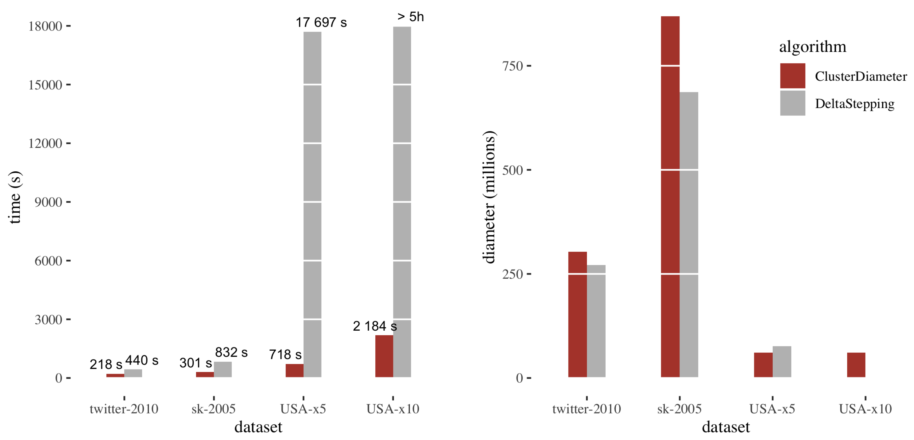
Figure 4 reports the comparison between
ClusterDiameter and
DeltaStepping on the benchmark datasets. The left plot shows running times, the right plot shows the diameter.
Considering the running times, we observe that on sk-2005 and twitter-2010 the running times are comparable, with ClusterDiameter being approximately twice as fast. Recall that DeltaStepping performs a number of parallel rounds linear in the unweighted diameter of the graph, whereas ClusterDiameter employs a number of rounds typically sublinear in this metric. However, on these two graphs the unweighted diameter is too small to make the difference in performance evident. On the other hand, USA has a very large unweighted diameter, and, as expected ClusterDiameter is much faster than DeltaStepping on this instance.
As for the diameter returned by the two algorithms, we have that both yield similar results, with ClusterDiameter reporting a slightly larger diameter on twitter-2010 and sk-2005. Note that DeltaStepping provides a 2-approximation, whereas ClusterDiameter provides a polylog approximation in theory. The fact that the two algorithms actually give similar results shows that ClusterDiameter is in practice much better than what is predicted by the theory. We notice that, since the very slow execution of DeltaStepping on USA-x10 was stopped after 5 hours, no diameter approximation was obtained in this case.
7.2. Behaviour of the Guessing of the Radius
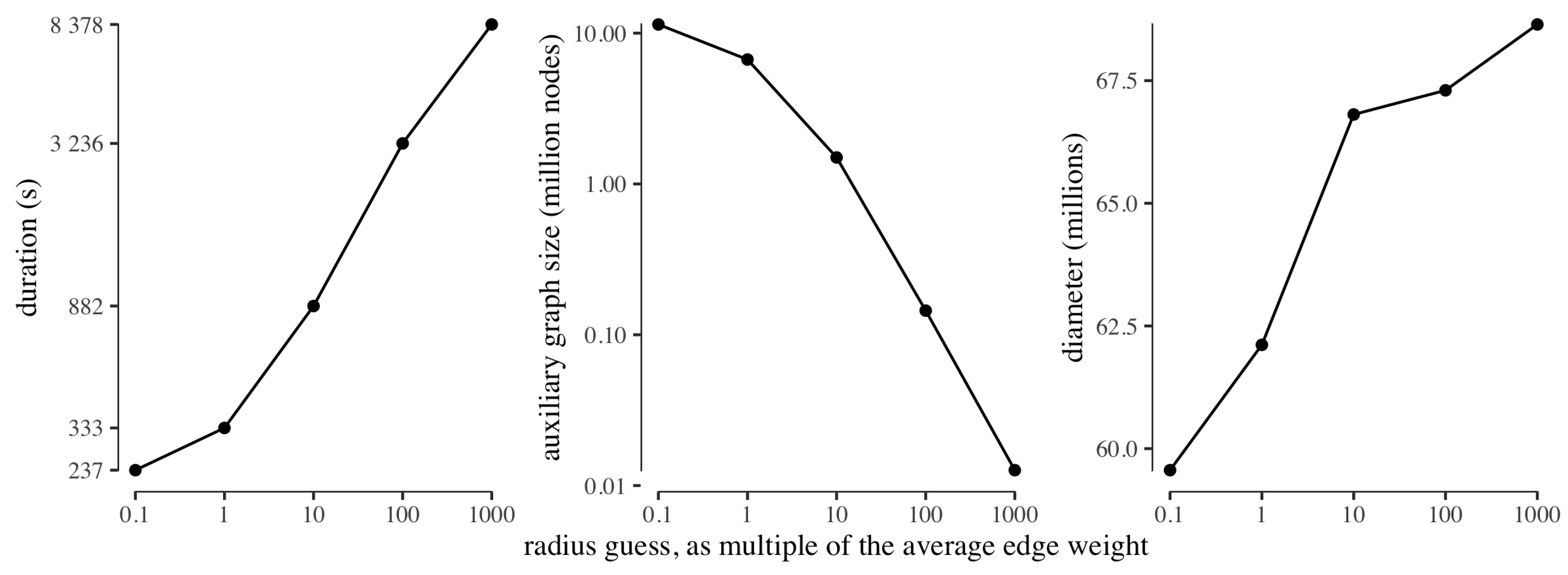
To test the behaviour of the guessing of the radius, we ran ClusterDiameter on USA with an initial guess of one tenth the average edge weight, increasing the guess by a factor ten in each step, and stopping at a thousand times the average edge weight. For each guessing step, we recorded the running time, along with the size of the auxiliary graph obtained with that radius guess, and the diameter approximation computed from the auxiliary graph. We remark that, in all experiments, the time required to compute the diameter on the auxiliary graph (not reported) is negligible with respect to the time required by the clustering phase.
Figure 5 reports the results of this experiment. First and foremost we note that, as expected due to exponential growth of the radius parameter in the search, the duration of each guessing step is longer than the cumulative sum of the durations of the previous steps. Also as expected, the size of the auxiliary graph decreases with the increase of the radius used to build the clustering. As for the approximate diameter computed from the different auxiliary graphs, intuition suggests that the auxiliary graph built from a very fine clustering is very similar to the input graph, hence will feature a very similar diameter; whereas a coarser clustering will produce an auxiliary graph which loses information, hence leading to a slightly larger approximate diameter. However, we observe that the diameter approximation worsens only slightly as the size of the auxiliary graph decreases (by less than
from the minimum to the maximum guessed radius). This experiment provides evidence that our strategy is indeed able to return good diameter estimates even on platforms where each worker has very limited local memory, although, on such platforms, the construction of a small auxiliary graph requires a large radius and is thus expected to feature large round complexity, as reflected by the increase in running time reported in the leftmost graph of
Figure 5.
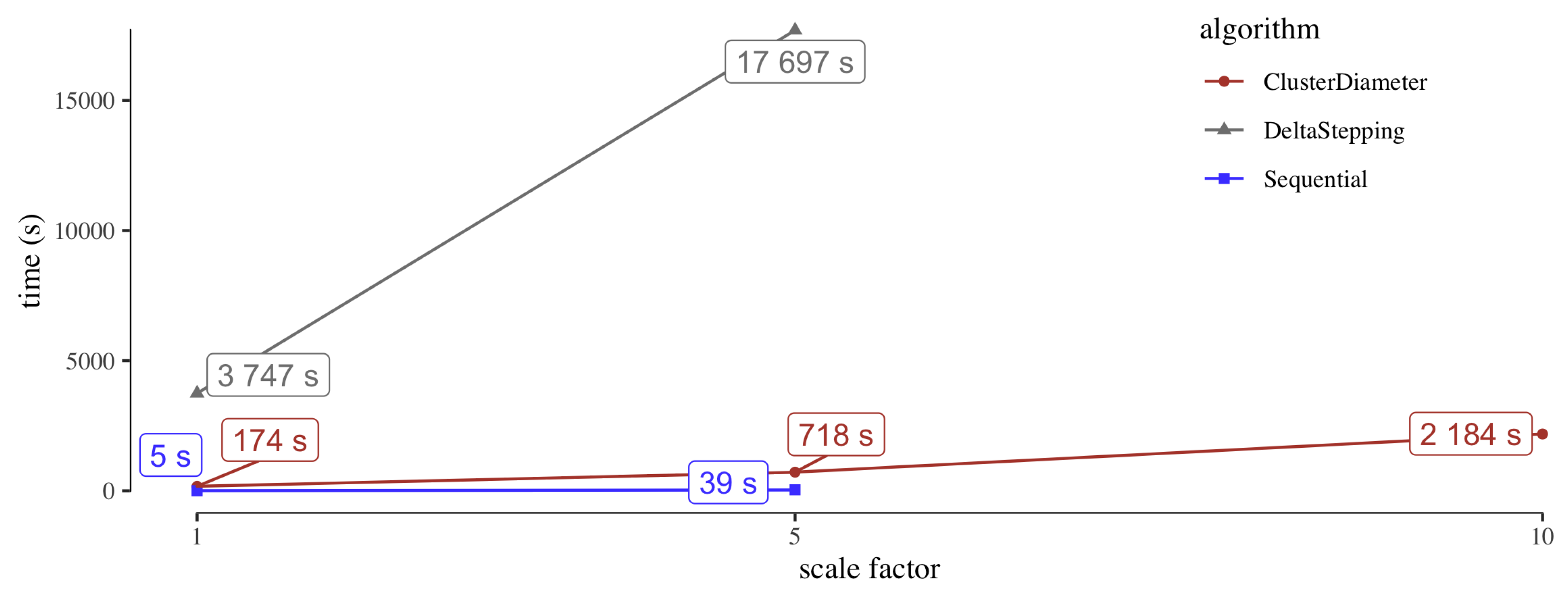
7.3. Scalability
The goal of the scalability experiments is twofold. One the one hand, we want to assess the overhead incurred by a distributed algorithm over a sequential one, in case the graph is small enough so that the latter can be run. On the other hand, we want to compare the scalability with respect to the graph size of ClusterDiameter versus DeltaStepping. To this purpose, we used as benchmarks the original USA network and the two inflated versions with . We note that both the original USA network and the inflated version with fit in the memory of a single machine. We did not experiment with the sk-2005 and twitter-2010 graphs, since it was unclear how to downscale them to fit the memory of a single machine, while preserving the topological properties. As a fast sequential baseline, we consider a single run of Dijkstra’s algorithms from an arbitrary node, which gives a 2-approximation to the diameter.
The results of the experiments are reported in
Figure 6. On the original
USA network, as well as on its fivefold scaled up version, the sequential approach is considerably faster than both
ClusterDiameter and
DeltaStepping, suggesting that when the graph can fit into main memory it is hard to beat a simple algorithm with low overhead. However, when the graph no longer fits into main memory, as is the case of
USA-x10, the simple sequential approach is no longer viable. Considering
DeltaStepping, it is clearly slower than
ClusterDiameter, even on small inputs, failing to meet the five hours timeout on
USA-x10, On the other hand,
ClusterDiameter exhibits a good scalability in the size of the graph, suggesting that it can handle much larger instances, even in the case of very sparse graphs with very large unweighted diameters.
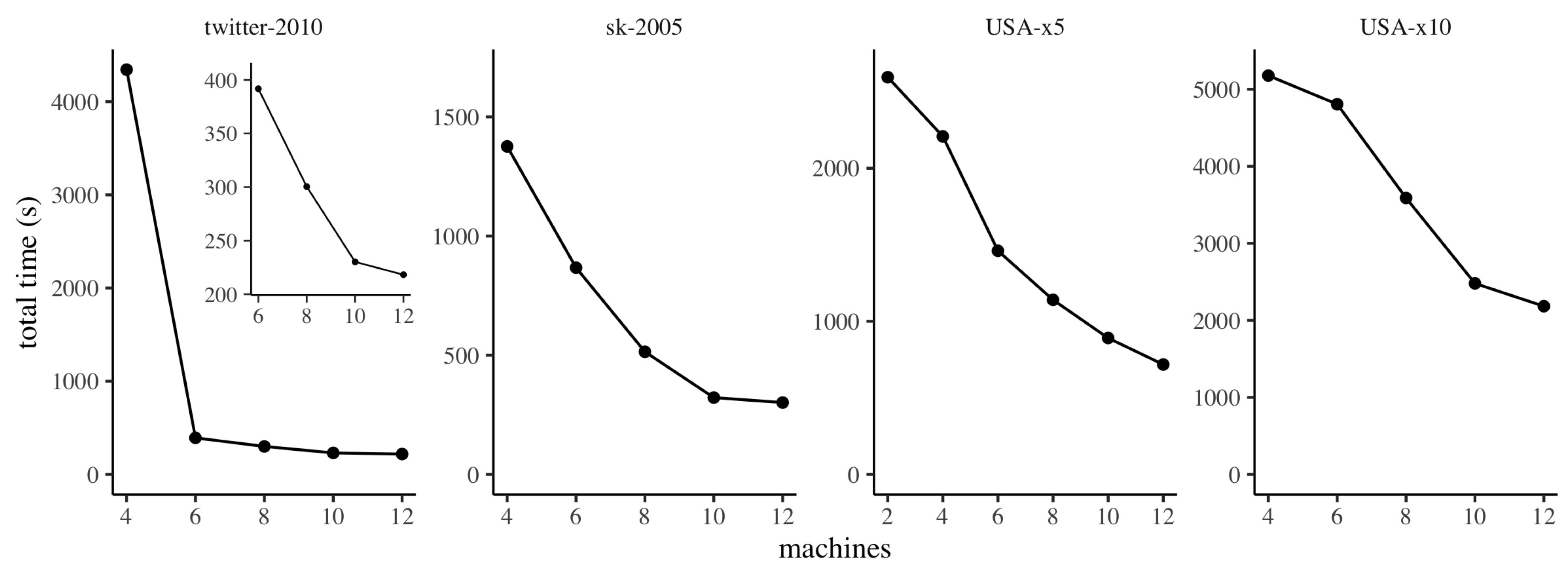
7.4. Strong Scaling
In this section we investigate the
strong scaling properties of
ClusterDiameter, varying the number of machines employed while maintaining the input instance fixed. The results are reported in
Figure 7, where, for each graph, we report results starting from the minimum number of machines for which we were able to complete the experiment successfully, avoiding running out of memory.
We observe that, in general, our implementation of ClusterDiameter scales gracefully with the number of machines employed. It is worth discussing some phenomena that can be observed in the plot, and that are due to peculiarities of our hardware experimental platform. Specifically, on twitter-2010 we observe a very large difference between the running times on 4 and 6 machines. The reason for this behaviour is that for this dataset, on our system, when using 4 machines our implementation incurs a heavy use of swap space on disk when building the clustering. Interestingly, the slightly larger graph sk-2005 does not trigger this effect. This difference is due to the fact that twitter-2010 exhibits faster expansion (the median number of hops between nodes is 5 on twitter-2010, and 15 on sk-2005), therefore on twitter-2010 the implementation needs to allocate much larger buffers to store messages in each round. From 6 machines onwards, the scaling pattern is similar to the other datasets, as detailed in the smaller inset plot. Similarly, on USA-x5, the scaling is very smooth except between 4 and 6 machines, where the improvement in performance is more marked. The reason again is that on 2 and 4 machines the implementation makes heavy use of swap space on disk during the construction of the auxiliary graph.
We remark that the experimental evaluation reported in this section focus exclusively on weighted graphs. A set of experiments, omitted for the sake of brevity, has shown that, on unweighted graphs of small diameter, a distributed implementation of BFS is able to outperform our algorithm, due to its smaller constant factors, while for unweighted graphs of higher diameter we obtained results consistent with those reported in this section for the weighted USA dataset.


