Abstract
Computing shortest-path distances is a fundamental primitive in the context of graph data mining, since this kind of information is essential in a broad range of prominent applications, which include social network analysis, data routing, web search optimization, database design and route planning. Standard algorithms for shortest paths (e.g., Dijkstra’s) do not scale well with the graph size, as they take more than a second or huge memory overheads to answer a single query on the distance for large-scale graph datasets. Hence, they are not suited to mine distances from big graphs, which are becoming the norm in most modern application contexts. Therefore, to achieve faster query answering, smarter and more scalable methods have been designed, the most effective of them based on precomputing and querying a compact representation of the transitive closure of the input graph, called the 2-hop-cover labeling. To use such approaches in realistic time-evolving scenarios, when the managed graph undergoes topological modifications over time, specific dynamic algorithms, carefully updating the labeling as the graph evolves, have been introduced. In fact, recomputing from scratch the 2-hop-cover structure every time the graph changes is not an option, as it induces unsustainable time overheads. While the state-of-the-art dynamic algorithm to update a 2-hop-cover labeling against incremental modifications (insertions of arcs/vertices, arc weights decreases) offers very fast update times, the only known solution for decremental modifications (deletions of arcs/vertices, arc weights increases) is still far from being considered practical, as it requires up to tens of seconds of processing per update in several prominent classes of real-world inputs, as experimentation shows. In this paper, we introduce a new dynamic algorithm to update 2-hop-cover labelings against decremental changes. We prove its correctness, formally analyze its worst-case performance, and assess its effectiveness through an experimental evaluation employing both real-world and synthetic inputs. Our results show that it improves, by up to several orders of magnitude, upon average update times of the only existing decremental algorithm, thus representing a step forward towards real-time distance mining in general, massive time-evolving graphs.
1. Introduction
Mining shortest-path distances is universally considered one of the most fundamental operation to be performed on graph data, due to the wide range of applications it finds. Prominent examples include social networks analysis [1], route planning [2,3], intelligent transport systems [4], context-aware search [5,6], web search optimization [7], graph databases [8,9], decision making [10], analysis of biological networks [11], artificial intelligence [12] and network design [13].
Standard algorithms for solving the problem of computing answers to queries on the distance, i.e., to retrieve the weight of a shortest path between a pair of vertices of a given graph upon request, are well known and include the Breadth First Search (BFS) algorithm for unweighted graphs and the Dijkstra’s algorithm for weighted ones. Unfortunately, there exists vast, mostly experimental, algorithmic literature showing they are not suited for solving the problem at large-scale, i.e., when the graph to be managed is massively sized [14,15,16,17]. In fact, in these cases, the mentioned approaches do not scale well enough against the input’ size, since their linear (or slightly superlinear for weighted graphs) worst-case time complexity yield impractical average time per query when graphs are huge (with up to millions of vertices and billions of arcs). The other extreme approach is to compute distances between all pairs of vertices beforehand and store them in an index [7]. Though in this way we can answer distance queries almost instantly, this approach is also unacceptable since preprocessing time and index size are quadratic and unrealistically large.
For the above reasons, and since big graphs are becoming the norm in most modern application contexts that rely on distance mining, many smarter and more scalable techniques, between these two extreme solutions, have been proposed in the recent past to deal with massive graphs. Essentially all of them adopt the common strategy of preprocessing the graph to compute some data structure that is then exploited to accelerate the query algorithm [2,3,7,9,18,19,20,21,22,23]. Some of these methods have been designed to handle special classes of graphs, of interest of specific applications (e.g., speed-up techniques for route planning) and in road/transport networks (e.g., [2,14,20,21,24,25]) while some others are general and provide speedups over baseline strategies regardless of the structural properties of the graph to be managed (e.g., [3,15,19,23]). In this latter category we find 2-HOP-COVER-based labeling approaches that currently are considered state-of-the-art methods for distance mining in massive graphs. In fact, they have been shown to exhibit superior performance in terms of query times, allowing computation of shortest-path distances in microseconds even for billion-vertex graphs, at the price of a competitive preprocessing time and space overhead [7,8,21,26,27].
Specifically, such approaches rely on the idea of precomputing a compressed representation of the transitive closure of the input graph in terms of concatenations of shortest paths: for each pair of vertices of the input graph, such representation includes (at least) one intermediate vertex, called hub vertex, and (at least) two corresponding shortest paths, connecting the hub vertex to the two vertices of the pair, called hops. In this way, the shortest path connecting the pair of vertices can be reconstructed as the concatenation of the two hops at the hub vertex. In more details, a label at each vertex contains the length of a shortest path towards each hub and, to retrieve the distance between two vertices, it suffices to find a common hub in their labels minimizing the sum of the two distances. The difficult point here is to find a small set of hubs covering a shortest path for each pair of vertices in the graph, since in this way the resulting labeling is compact and, consequently the average query time is small. Indeed, it is known that finding a minimum size set of hubs is NP-hard [18,28] but both heuristics and approximation algorithms, for computing fairly compact labelings, providing excellent practical performance in terms of query times at the price of a reasonable preprocessing effort, are known [3,7,18]. Specifically, the two approaches of [3,7] currently are considered the best options in this direction.
A further level of complexity arises when the network to be handled is time-evolving, i.e., is when the underlying graph can evolve over time. In fact, in this which is universally considered the most realistic scenario, every time the network is subject to an update, i.e., when the corresponding graph undergoes some topological change (e.g., an arc removal or an arc weight decrease), the preprocessed data can become obsolete and hence must be updated to preserve query correctness (i.e., that exact distances are returned). A naive way to produce updated preprocessed data is to recompute everything from scratch. Nonetheless, this is not a practical strategy when inputs are massive, as it requires unsustainable computational overheads [8,27,29]. Observe that this issue is common to many preprocessing-based approaches for mining properties from big graphs (e.g., mining betweenness centralities [30]).
For these reasons, in the last few years, researchers have worked to adapt known methods, for mining (generic) properties from static graphs, to function in such time-evolving scenarios through the design of specific dynamic algorithms, i.e., algorithms that are able to update the preprocessed data to reflect graph changes without performing any full recomputation from scratch [8,14,17,24,25,26,27,30,31]. Such algorithms are typically divided in two broad categories, namely incremental and decremental algorithms, depending on whether they able to handle incremental updates only (i.e., insertion of vertices/arcs and arc weight decreases) or decremental updates only (deletion of vertices/arcs and arc weight increases).
Both types of algorithms find several prominent applications in the real-world, as well documented in the literature [8,17,26]. On the one hand, incremental algorithms are essential to handle scenarios where the graph to be managed tends to be subject to sequences of changes that correspond to a growth of the size of the underlying network. Examples include citation networks, where new references or new authors can be added dynamically, or email/messaging networks, where one can observe only new emails being sent and new addresses being added. On the other hand, decremental algorithms are useful in all those cases where the graph to be managed tends to be subject to sequences of changes that correspond to a reduction of the size/functionality of the underlying network. Examples include: communication networks where links can become unavailable, and arc weights representing latencies typically can deviate by increasing from the initial value; railway/bus networks where delays due to disruptions can occur, while no train is allowed to leave before the scheduled time; data mining for linked data (web link analysis, social network analysis, biological networks analysis, databases processing) where one’s purpose is to determine which nodes/links are the most important by observing the effect of removals/congestions on the structure of the shortest paths (and/or diameter or components) of the corresponding graphs. Finally, it is well known that both kinds of solutions are necessary to build effective fully dynamic algorithms that are of fundamental importance for all those applications where the structure of the sequences of modifications, affecting the graph, is unpredictable [26,32,33]. A typical example is social network analysis where users can join or leave, and connections between users can be established or removed.
For all above reasons, it is of utmost importance to have efficient algorithms to process both incremental and decremental operations when one aims at mining shortest-path properties from a time-evolving graph. Please note that the investigation on dynamic algorithms can also have a general graph theoretical interest since, often, studying how decremental changes affect shortest paths can also have applications to static graphs problems or other contexts (see, e.g., works on multi-commodity flows or cut problems [34]).
1.1. Our Contribution
For 2-hop-cover labelings, two dynamic algorithms that do not compromise on query performance are known, both employing the common strategy of identifying and updating only the part of the labeling that is compromised by a graph change. In details, the algorithm proposed in [8], named resume–2hc, is able to handle incremental updates only while the algorithm proposed in [26,27], named bidir–2hc, can manage decremental updates only. Both have been shown, experimentally, to be rather effective and faster on average than the recomputation from scratch and to preserve the quality of the labeling in terms of query time and compactness (while there exists a dynamic approach that tolerates degradation on query time to achieve fast update [31]). Moreover, both have been combined and tested as a single fully dynamic algorithm in [26]. However, while the former exhibits extremely low update times that are compatible with real-time applications, the latter is slower, and sometimes only slightly better, on average, than the recomputation from scratch in some categories of input instances that are highly relevant to application domains, e.g., sparse weighted graphs.
In this paper, we focus on this latter issue and try to overcome the above limiting factor of bidir–2hc by introducing a new dynamic algorithm, called queue–2hc, to update 2-hop-cover labelings when decremental update operations affect the input graph. We prove its correctness and formally analyze its worst-case performance. Since its worst-case time complexity cannot be directly compared with that of bidir–2hc, which depends on different parameters, we assess its effectiveness through an extensive experimental evaluation employing both real-world and synthetic inputs. Our results show that queue–2hc improves, in some case up to orders of magnitude, upon the update times of bidir–2hc, especially in some input categories where such algorithm was shown to be not so effective. Our results also show queue–2hc is always much faster than the recomputation from scratch, despite being worse in terms of worst-case complexity. This is a feature in common with bidir–2hc and resume–2hc, have been observed to be very effective in practice, despite their worst-case bound on the running time. The same holds for the preprocessing method, which is much faster in practice than what the worst-case bound suggests. This is a quite common behavior in the field of research dedicate to dynamic algorithms, typically due to two main reasons: either the worst-case essentially never or very rarely occurs in practical cases, or that the analysis is not tight. Nonetheless, having solutions like the one proposed in this paper is necessary to allow the use of the 2-hop-cover labeling method in the real-world. Thus, to summarize, queue–2hc can be considered a step forward towards real-time distance mining for general, massive time-evolving graphs.
1.2. Structure of the Paper
The paper is organized as follows. In Section 2 we give the notation and nomenclature used throughout the manuscript, describe the basics of the 2-hop-cover labeling technique, and the algorithms known in the literature for handling the time-evolving scenario. In Section 3 we introduce our new algorithm, sketch its correctness proofs and computational complexity analysis while in Section 4 we present the experimental evaluation we conducted to assess the performance of the new approach. Finally, Section 5 concludes the paper and outlines possible future research directions.
2. Notation and Background
In this section, we provide the notation and the background notions that are necessary to introducing the contributions of the paper. In the remainder of the paper, for the sake of simplicity and generality, we consider the most general setting where the graph to be handled is a directed weighted graph , with vertices and arcs, such that is a weight function assigning a positive real to any arc .
A path in G, connecting two vertices s and t, is a sequence of arcs where , , and each consecutive pair of arcs in the sequence shares a common endpoint. We call k the length of the path itself, i.e., the number of arcs in the sequence. A path is simple if it does not contain self-loops, i.e., if any vertex in the sequence of arcs appears only once. Moreover, we denote by the weight of a path P, defined as the sum of the weights of its constituting arcs, i.e., . A path P, connecting two vertices u and v, that has minimum weight among all paths in G between said two vertices is called a shortest path from u to v. We call the distance from vertex u to vertex v in G, which is the weight of a shortest path from u to v in G. If such a path does not exist, i.e., vertices are disconnected, then we assume . Observe that conventionally, in unweighted graphs we have for all . Therefore, the weight of a shortest path equals its length in these graphs.
We denote by (, respectively) the set of the outgoing (incoming, respectively) neighbors of v in G, that is (, respectively). Clearly, in undirected graphs we have for any . Furthermore, we denote by the transpose of G where an arc if and only if , and . Similarly, we use (, respectively) to denote the set of the outgoing (incoming, respectively) neighbors of v in . A graph update or modification can be either incremental, if it is an insertion of a new arc or a decrease in the weight of an existing arc, or decremental, if otherwise it is a deletion or an increase in the weight of an existing arc. Please note that insertions/deletions of arcs can be easily modeled as decreases of weights from ∞ to and vice versa. Notice also that vertex insertions/deletions can be easily modeled as sets of modifications to the corresponding arcs, hence the approaches for handling arc updates can be easily extended to manage vertex insertions/deletions by repeatedly executing them for the set of adjacent arcs. For the sake of clarity, we use to represent the distance function in a given graph G but we omit subscripts from our notation whenever the meaning is clear from the context.
2.1. 2-hop-cover Labeling
In this section, we summarize the main characteristics of the 2-hop-cover labeling method. Our descriptions refer to the most general case of weighted directed graphs, which is the most complex to handle. Simpler versions of the approaches can be obtained for unweighted or undirected graphs, we refer the reader to [26] for a thorough discussion on the differences.
For each vertex v of G, we call incoming and outgoing labels, respectively, and of v two sets of pairs (also known as label entries) of the form and , respectively, where while and , respectively. The collection of all the labels is referred to as a distance labeling of G. For the sake of readability, we use (, respectively) to denote that (, respectively), whenever the meaning is clear from the context. Similarly, for any we say whenever there exists some such that and (and vice versa). Labels can be used to retrieve the (exact or approximate) distance from vertex to vertex in G by performing a query on the distance from s to t, as in Equation (1).
Please note that each query requires access to the labels of s and t only.
A distance labeling L is a 2-hop-cover labeling [18] of a graph G (often referred to simply as labeling of G in the remainder of the paper) if, for any pair of vertices :
- either contains (at least) a vertex lying on a shortest path between s and t in G, and therefore (s and t are connected in G);
- or and hence (when s and t are not connected in G).
If a pair of vertices is connected, then the above-mentioned vertex , lying on a shortest path from s to t, is called hub vertex of pair (or simply hub). Vertex h is said to cover pair . Symmetrically, the pair is said to be covered by h and, thus, by the labeling L. By extension, if the above conditions hold, the graph is said to be covered by the labeling and the labeling is said to cover the graph (or to satisfy the cover property for the considered graph). Notice that a given pair of vertices can be covered by more than one hub vertex, depending on how the 2-hop-cover labeling is computed.
A naive approach to compute a 2-hop-cover labeling of a graph consists of executing twice a shortest-path algorithm that can be a Breadth First Search (BFS) in unweighted graphs or the Dijkstra’s algorithm in weighted ones, using as root each vertex , once forward (that is, in G), and once backward (that is, in ). In the forward case, when a vertex u is extracted from the queue, used by the shortest-path algorithm, with a priority of d, that is when a shortest path with weight d from the root v to u in G is found, then entry is added to . In the backward case, instead, entry is added to whenever vertex u is extracted from the queue and hence when a shortest path, with weight d, from the root v to u in , is found.
It is easy to see how a labeling obtained as above covers the graph [7], since there is at least one hub vertex per pair of vertices (the root vertex of each visit). However, computing a labeling L as above costs worst-case time, where is the worst-case computational time of a corresponding shortest-path algorithm. Moreover, L contains hub vertices and hence label entries, which is the same space complexity of storing all pairs distances. Furthermore, it induces a query algorithm with computational effort, since all labels contain entries. Thus, this basic version of 2-hop-cover labeling is far from being considered an effective approach for distance mining, since, as is, it is worse than standard methods for shortest paths. To make it practical, one must aim at minimizing both running times for computing a labeling (a.k.a. preprocessing times) and labeling size (i.e., total number of entries), which in turn hopefully induces small query times in practice.
To this end, unfortunately, it is known that finding a minimum-size labeling covering a graph G is an NP-hard problem [18]. However, few heuristic approximation algorithms for computing compact labelings are known [3,7,18].
In particular, the ones in [3,7] have been shown to achieve considerably better scalability, in terms of both preprocessing times and space requirements, than other methods in essentially all classes of graphs. Both these methods require worst-case running time to compute a labeling that can have label entries. Nevertheless, extensive experimentation shows they behave very well in practice. Specifically, they exhibit preprocessing times in the order of hours even for massively sized inputs, and produce labelings that have a labeling size that on average, is much smaller than the worst-case estimation of a constant multiple of [3,7]. This leads to have average query times that in practice, are below milliseconds even for the largest instances.
The elements that are common to the two strategies are: (i) considering the vertices of V in order according to some importance criterion with respect to the shortest paths in the graph; (ii) performing a number n of shortest-path visits, each rooted at a vertex in the above-mentioned order, say , that incrementally build the labeling starting from empty label sets (Observe that the ordering can be greedily changed in this phase to achieve better results); (iii) employing a so-called pruning mechanism that stops the branch of the graph that is currently being explored whenever a pruning condition is met. In particular, let us denote by the vertex ordering and by the labeling computed after the execution of the two shortest-path visits, rooted at vertex (i.e., containing only entries of the form for ).
If we consider a vertex u that is reached during the forward (backward, respectively) visit rooted at and assume that is the currently discovered distance from to u (from u to , respectively). Then, the algorithm checks whether (, respectively). If the above condition holds, then already contains a hub vertex for pair (, respectively) and for all pairs such that there exists a shortest path between and x passing through vertex u (for all pairs such that there exists a shortest path from x to passing through vertex u, respectively). Therefore, the visit rooted is pruned at u. Otherwise, the algorithm updates either or as described above and continues. Clearly, for each vertex u that is not reachable from (that cannot reach , respectively), we have (, respectively). It can be proven that the obtained is a 2-hop-cover labeling [7]. It can also easily seen that both methods guarantee that if in the considered vertex ordering, then both and , while v might be in or in . This property, called well-ordering property [22], is quite important, as it can be exploited to prove that the computed labeling is minimal [7], in the sense that removing any single label entry from the labeling breaks (i.e., induces the violation of) the cover property for at least one pair of vertices of the graph. Formally speaking, the well-ordering property is as follows.
Property 1
(Well-ordered Labeling). Let be a 2-hop-cover labeling of a graph . Let be an ordering on the vertices of G. Then L is well-ordered if, for any such that we have that:
- ;
- and .
Please note that minimality is a highly desirable property since it has been empirically shown that 2-hop-cover labelings that are minimal and that are computed by considering certain vertex orderings yield excellent practical performance in terms of both preprocessing time, labeling size, and average query times. In particular, it is known that the performance of the methods above heavily depends on the vertex ordering and it has been experimentally observed that the average label size (and the resulting average running time of the query algorithm) decreases by several orders of magnitudes, with respect to random orderings, if vertices are sorted according to a centrality-related measure, like, e.g., vertex degree or (approximations of) betweenness centrality [3,7,26]. Moreover, for well-ordered (minimal) labelings, if distinct ids ranging from 0 to are assigned to the vertices of V and, for each vertex , pairs in and are stored in the form of an array and sorted according to said ids, then can be effectively implemented as shown in Algorithm 1 to take worst-case running time ( and denote the number of label entries in the two labels). Given a label, say , of a vertex v stored as above, in what follows we denote by it i-th element and by its size.
| Algorithm 1: Query algorithm for minimal well-ordered labelings |
 |
In the remainder of the paper, we will call fs–2hc the generic preprocessing strategy, described above, that yields well-ordered minimal labelings.
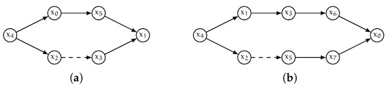
Observe that all dynamic algorithms known can be used regardless of the specific preprocessing strategy used to compute the initial labeling of the graph [7,26]. We will show that the same holds for the new algorithm proposed in this work. More specifically, all dynamic algorithms considered in this paper only need an initial labeling that is well-ordered, and this is guaranteed if fs–2hc strategies are used. A sample directed, unweighted graph, with a corresponding well-ordered minimal 2-hop-cover labeling is shown in Figure 1.
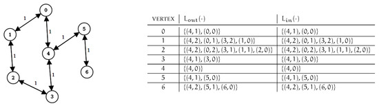
Figure 1.
A sample graph and a corresponding 2-hop-cover labeling is shown. Vertex ordering is .
2.2. Dynamic Algorithms for Updating 2-hop-cover Labelings
Essentially, the only two known methods for updating 2-hop-cover labelings are those in [8,26], named resume–2hc and bidir–2hc in what follows, respectively, whose main features are briefly summarized below, since the new approach we propose in this paper borrows some features from both solutions. We refer the reader to [8,26] for a thorough description of the resume–2hc and bidir–2hc, respectively.
Algorithm RESUME–2HC. Given a graph and a 2-hop-cover labeling L of G, algorithm resume–2hc is able to update L in order to reflect an incremental update (i.e., a newly added arc or a decrease in the weight of an arc ). In particular, if we denote by G a graph before a given incremental modification, by L a 2-hop-cover labeling L of G, and by the graph resulting by the application of the change to G, then resume–2hc computes a 2-hop-cover labeling of by updating L as follows.
First of all notice that resume–2hc does not remove from L the so-called outdated label entries of L, i.e., entries in the label sets that correspond to shortest paths in G but not in , due to the incremental update occurred on arc , and hence they are present also in . Formally, an outdated entry is a pair (or symmetrically ), for some u and v in G, such that (or symmetrically ). The above choice is motivated by the fact that distances can only decrease as a consequence of incremental updates and hence, if one adds entries corresponding to new shortest paths, then queries return correct distances in for all pairs of vertices even in the presence of such outdated entries (i.e., the cover property is preserved). This is because the query algorithm searches for minimum values in the label sets.
Therefore, resume–2hc simply adds new label entries or overwrite distances of existing ones. A drawback of this approach is that the minimality of the resulting labeling as a whole is broken even after a single update and this is known to affect the performance over time (periodical reprocessing is necessary to restore minimality and avoid the labeling grows too large). Observe that the problem of designing an incremental algorithm that does not suffer from this issue is still open [29].
The strategy of resume–2hc, for adding label entries corresponding to new shortest paths, is based on the following two facts: (i) if the distance from a vertex to a vertex u changes, then all new shortest paths from to u pass through the updated arc ; (ii) if a shortest path P from to changes, then the distance between and w changes, where w is the penultimate vertex in P. Based on the above insights, for every vertex , the idea is that it suffices to resume forward and backward, respectively, shortest-path visits (i.e., in and , respectively) that: (i) are originally rooted at ; (ii) start at b and a, respectively; (iii) stop at unchanged vertices. That is, instead of inserting into the priority queue, the algorithm inserts pair (, respectively). Then, the search proceeds by adopting a pruning mechanism similar to that of fs–2hc described above, modified to consider that outdated entries are not removed. In particular, it employs the notion of prefixal query, denoted as pQ, that, given two vertices and an integer k and a labeling L, is computed as in Equation (2).
In simpler terms, is the answer to a query from s to t computed from labeling L using distances to vertices only. Suppose now a resumed forward (backward, respectively) visit, originally rooted at , visits vertex u with distance , then it is possible to prune the search at u if (, respectively). It can be shown that to obtain a 2-hop-cover labeling of by updating L with the above strategy, it suffices to resume forward and backward shortest-path searches rooted at vertices [8].
Algorithm BIDIR–2HC. First of all, notice that when handling a decremental graph update, outdated label entries must be removed from L to obtain a 2-hop-cover labeling of , as otherwise it is easy to show the cover property does not hold for . Specifically, even after a single decremental operation, a query on such labeling might return an arbitrary underestimation of the true value of distance in . For this reason, algorithm bidir–2hc works in three phases. If we assume that an arc undergoes a decremental update (i.e., either it is removed or its weight is increased), in a first phase bidir–2hc performs two shortest-path-like searches of the graph G, one backward (i.e., on ) and one forward (i.e., on G itself), rooted at x and y respectively. By exploiting both L and the structure of the graph, the visits detect the so-called affected vertices, i.e., vertices that are candidate to contain at least one outdated label entry. In a second phase, the algorithm scans all such vertices and removes outdated label entries. For efficiency purposes, affected vertices are divided into two sets and are sorted according to the original vertex ordering, and the removal policy works as follows: (i) given an affected vertex v of the first set, entries such that u is in the second set are removed from (if any); (ii) given an affected vertex v of the second set, entries such that u is in the second set are removed from (if any). The result of the removal phase is that there might be pairs of affected vertices that are not covered by the resulting labeling, depending on the structure of . Therefore, a third phase to restore the cover property for all such pairs is executed to obtain a labeling that covers . To this aim, a set of shortest-path searches is performed, namely one forward search in , rooted at each affected vertex of the first set, and one backward search in , rooted at each affected vertex of the second set, following the vertex ordering to achieve both the well-ordered property and the minimality. Such visits essentially discover shortest paths connecting pairs of affected vertices and, accordingly, add entries to the corresponding labels. As well as both fs–2hc and resume–2hc, a pruning mechanism is incorporated in these visits, based on the ordering of vertices and on results of queries. However, the pruning is less “aggressive” and hence less effective in reducing the search space in practice. The motivation is essentially that shortest paths, connecting affected vertices in or , can pass through non-affected vertices (see [27,29] for more details). Therefore a forward (backward, respectively) visit, rooted at affected vertex of the second (first, respectively) set, can be stopped only if (or , respectively) and u is an affected vertex of the first (second, respectively) set, where is the distance from to u (from u to , respectively) found by the visit and is the labeling restricted to entries of the form for .
3. A New Algorithm: queue–2hc
In this section, we describe our new decremental algorithm for updating 2-hop-cover labelings, named queue–2hc. Our description refers to the most general case of weighted directed graphs, which is the most complex to handle [3,8,26,27]. Simpler versions of the approaches can be easily obtained for unweighted or undirected graphs by considering the observations reported in the previous sections or in [8,26,27].
3.1. Profiling of Algorithm bidir–2hc
The new method is inspired by some empirical observations on the behavior of bidir–2hc, the only previously known solution for updating 2-hop-cover labelings against decremental graph changes. These observations come from a preliminary experimental study we conducted through profiling software on an implementation of bidir–2hc itself. Specifically, our data show that:
- the first two phases require typically small fractions of the time taken by bidir–2hc, even in very large instances. However, some “computational redundancy” is observed. In particular, there can be some vertices whose label sets do not contain any outdated entry and yet such sets are scanned twice, once during the detection phase and once during the removal phase (within the computed set of affected vertices, see [26] or Section 2.2). This is clearly an undesired behavior that we aim at removing by designing a new algorithm for the purpose. An example of this scenario is shown in Figure 2.
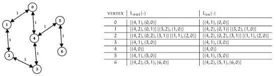 Figure 2. Consider the graph of Figure 1 (left) and the corresponding labeling (right). Assume arc is removed. If Algorithm bidir–2hc is executed, vertices have their label sets scanned twice, once during the detection of affected vertices and once during the removal phase, since hub vertex for pairs , and is vertex 4. However, no label entry is removed from nor from (the same hold for label sets of , , , ). Our algorithm instead scans these label sets only once.
 - the largest fraction of the entire computational effort to update a labeling, as a consequence of a decremental update, is spent by bidir–2hc on testing whether the cover property is satisfied and in restoring it when it is not, i.e., on the third phase. During this step, a number of shortest-path driven visits of the graph is performed, each rooted at one of the mentioned affected vertices and pruned according to a policy that is similar to that of fs–2hc. Unfortunately, however, the pruning conditions are less restrictive with respect to those of fs–2hc. Specifically, during the search started at , whenever a vertex u is settled with a distance of , the algorithm checks whether and prunes the search in the affirmative case, since this implies that labeling contains a hub vertex for and for all pairs such that there exists a shortest path between and x passing through node u. On the contrary, bidir–2hc must consider the fact that new paths, connecting pairs of affected vertices, can pass through non-affected vertices. Hence, to guarantee that the cover property is restored for all pairs of vertices, the search is pruned only if and u is affected. A consequence of this strategy is that many vertices of the graph, whose label sets do not change, are visited and tested for pruning by the searches of the third phase. This is, again, an undesired behavior we aim at avoiding by our new solution.
Beyond the Limitations of IDIR–2HC. Our algorithm tries to overcome the above-mentioned limitations by attacking the problem in a different way with respect to bidir–2hc. In details, the algorithm works in two phases, named clean and recover, respectively, as summarized in Algorithm 2. The aim of the clean phase is two-fold: (i) that of identifying and removing outdated label entries efficiently from the labeling (to produce an updated version of the labeling that contains only entries that are correct for the new graph); (ii) that of determining pairs of vertices that remain uncovered by the removal of outdated label entries without scanning their label sets twice (as done by bidir–2hc). The recover phase’s purpose, instead, is that of restoring the cover property for such pairs by suitably adding new label entries without visiting vertices of the graph whose label sets are unchanged by the graph update (unlike bidir–2hc). The two phases are described in the following sections.
| Algorithm 2: Algorithm queue–2hc |
| Input: Graph G, 2-hop-cover labeling L of G, arc subject to decremental update. Output: Resulting graph , 2-hop-cover labeling of .
|
3.2. clean Phase
Given an arc that undergoes a decremental update, the clean phase aims at performing a more efficient regarding bidir–2hc, removal of outdated labels, by finding and removing all and only outdated label entries (from now on simply referred to as outdated entries) from the labeling, i.e., by avoiding to remove any correct entry. This is obtained by scanning the labels of vertices that are actually subject to entry removals and, contextually, by identifying pairs of vertices that might remain "uncovered" (i.e., without an hub in the labeling) after the removal of the mentioned incorrect label entries. This last identification step is necessary to test that the cover property for the new graph efficiently, in a next phase. The two purposes above are achieved, in detail, by:
- determining two sets of vertices, named forward invalid hubs and backward invalid hubs, respectively, that are hubs for some pair in G but might stop being hubs in , due to the operation on , so to remove from L the incorrect entries associated with such vertices;
- identifying and exploring two (virtual) subgraphs of the input graph, named forward cover graph and backward cover graph, respectively, and denoted by and , respectively
In more details, to define our algorithm we give the following definitions.
Definition 1
(Forward Cover Graph). Given a graph , a 2-hop-cover labeling L of G, an arc . The forward cover graph is a subgraph of G with and as vertex and arc sets, respectively, as follows:
- a vertex u is in if and there exist two pairs and such that (that is a shortest path from u to y includes and h is a hub vertex for pair );
- an arc is in if and (hence ).
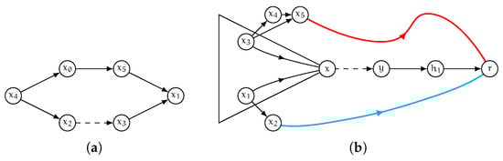
In other words, vertices of the forward cover graph are those with, in G, a shortest path toward y that might contain arc and hence whose distance toward y might change as a consequence of a decremental operation occurring on . Please note that whether the distance toward y changes or not depends on the number of shortest paths from the vertex to y that are in the graph, and on the vertex ordering (see Figure 3a for a graphical example of two different vertices of the forward cover graph). Note also that the arcs of such graph are the arcs of a shortest-path arborescence of G rooted at x plus arc . Symmetrically, we define a backward version of the cover graph as follows.
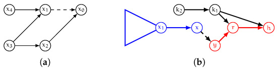
Figure 3.
(a): assume all arcs in this example have unitary weight and the vertex ordering is . Both and are in since the hub vertex for pairs and , in the labeling L induced by the above ordering, is vertex . However, if arc is removed then changes while does not, since has two shortest paths of the same weight to . (b): In the toy graph G shown here the only shortest path from x to h passes through arc . Therefore, if undergoes a decremental update, we have that , and all vertices that are connected to , are in the forward cover graph (in blue). Symmetrically, r and h are in the backward cover graph (in red) while and are in neither of the two cover graphs.
Definition 2
(Backward Cover Graph). Given a graph , a 2-hop-cover labeling L of G and an arc . The backward cover graph is a subgraph of G with and as vertex and arc sets, respectively, as follows:
- a vertex u is in if and there exist two pairs and such that (that is a shortest path from x to u includes and h is a hub vertex for pair );
- an arc is in if and (hence ).
In other words, analogously to the forward case, vertices of the backward cover graph are those having, in G, a shortest path from x that might contain arc and hence whose distance from x might change as a consequence of a decremental operation occurring on . Please note that again whether the distance from x changes or not depends on the number of shortest paths from the vertex from x that are in the graph, and on the vertex ordering. Note also that the arcs of such graph are the arcs of a shortest-path arborescence of rooted at y plus arc (a toy example of the structure of cover graphs for a given input graph is shown in Figure 3b).
Finally, we define the set of forward invalid hubs (backward invalid hubs , respectively) of as follows.
Definition 3
(Forward Invalid Hubs). Given a graph , a 2-hop-cover labeling L of G and an arc . Then, the set of forward invalid hubs of is defined as:
Similarly, we give a backward version.
Definition 4
(Backward Invalid Hubs). Given a graph , a 2-hop-cover labeling L of G and an arc . Then, the set of backward invalid hubs of is defined as:
Given the above definitions, algorithm clean’s strategy is based on the following properties. Notice that for the sake of simplicity, in what follows we use or to denote a vertex v belonging to the vertex set of either the forward or the backward cover graph.
Property 2.
Let L be a 2-hop-cover labeling of G. Assume arc is subject to a decremental operation and let be the graph obtained by applying to G such modification. Let (, resp.) be the forward (backward, resp.) cover graph. Then, for any vertex such that (, resp.) we have that (, resp.) contains only correct entries for , that is for any we have (for any we have , resp.).
Proof.
By definition of forward cover graph, we know implies there does not exist two pairs and such that for some . Observe that for any 2-hop-cover labeling, , for some , implies . Now, by contradiction, assume an entry is outdated, that is . This implies that the only shortest path from u to y in G includes arc (since the update is decremental we have that increases) and h is a hub vertex for pair . Hence we would have u is in the forward cover graph since there exist pairs and such that , which is a contradiction. The proof for the backward version is symmetric. □
Corollary 1.
For any pair such that and , we have that labeling L covers the pair also for , that is .
Proof.
Consider that for any pair , since L is a 2-hop-cover labeling, we have . Moreover, having and implies both and contain only correct entries for . Therefore . □
Hence, regardless of the magnitude of the change on , we are sure that the cover property is satisfied by L also in , for pairs such that and and we do not need to search for outdated entries in outgoing labels of vertices of the forward cover graph nor in incoming labels of vertices of the backward cover graph.
Now, we establish how to determine which entries are outdated in the labels of the vertices of the two cover graphs. Please note that there can be labels of vertices of the two cover graphs that do not contain outdated entries. Still, we will show it is necessary to identify such vertices since they might be interested by violations of the cover property due to the removals of the above-mentioned outdated entries. This heavily depends on the structure of the shortest paths in the graph and on the effect of the decremental update on such structure, as shown in the example of Figure 4.
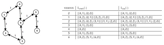
Figure 4.
Consider again the graph of Figure 1 and a corresponding 2-hop-cover labeling. Assume arc is removed. We have that vertex 3 is in and vertex 0 is in . However, there is no outdated label entry in but the decremental operation on arc causes the cover property to be broken for pair .
Property 3.
Let and be the forward and backward cover graphs, respectively. Let L be a well-ordered 2-hop-cover labeling of G. Assume arc is subject to a decremental operation and let be the graph obtained by applying to G such modification. Let and be the sets of forward and backward invalid hubs. Then:
- a label entry in the outgoing label of a vertex is outdated if and only if and there is no vertex such that: (i) ; (ii) ; (iii) ;
- a label entry in the incoming label of a vertex is outdated if and only if and there is no vertex such that: (i) ; (ii) ; (iii) .
Proof.
We focus on case 1. The proof for case 2 is symmetric.
(⇒) First of all observe that if contains an outdated label entry then, by Lemma 2, we must have and hence we know that and , i.e., v is connected in G to y via a shortest path that includes . By contradiction, we now assume that is outdated but one of the two following conditions is true:
- ;
- and there is a vertex such that: (i) ; (ii) ; (iii) .
Case 1. If , we have that h is not a hub vertex for pair in L. This implies that there exists another hub vertex that covers pair which in turn implies that:
- either ;
- or but h is not hub vertex (that is h does not belong to ) since precedes both h and x in the vertex ordering ( and ) and since L is well-ordered.
In both sub-cases we obtain a contradiction, as is not outdated (the decremental operation does not change the value of ).
Case 2. We have that there exists a neighbor of v, namely u, that is not in . Hence, its outgoing label, by Property 2, does not contain any incorrect entry and we have for any . Therefore, as and the weight of does not change in , we have that and thus the label entry is not outdated, which is a contradiction.
(⇐) Again by contradiction we assume that there is a non-outdated (correct) entry while and there is no vertex such that: (i) ; (ii) ; (iii) . Since and we know that . Now, since the entry is correct for , there must exist another shortest path, say P, in G that: (i) does not contain and such that . Call the neighbor of v on this second shortest path. Since there is no neighbor u such that and , it follows that .
It follows that pair is covered by some other vertex, say , such that and . Since we have also that h must be preceding in the vertex ordering (i.e., ) as otherwise the visit rooted at h would have not reached v (it would have been pruned thanks to ). This is a contradiction since for the pruning on P to happen must precede h. An explanatory example of this scenario is shown in Figure 5a. □
Figure 5.
(a): an example of the contradiction reached in the proof of Property 3. Suppose vertex ordering is and all arcs weight 1 for the sake of the example. Therefore, in any minimal well-ordered 2-hop-cover labeling entry cannot belong to . This allows Algorithm clean to avoid removing correct entries. (b): a case where a correct entry is preserved by Algorithm clean. Suppose the vertex ordering is and all arcs weight 1 for the sake of the example. Therefore in any minimal well-ordered 2-hop-cover labeling, will contain with . Clearly, also and will contain. similarly, entries and , respectively. If arc undergoes some decremental update, the (correct) entry in is not removed thanks to the presence of the alternative shortest path through with the same weight as that through .
To summarize, Properties 2–3 provide a theoretical basis upon which we design an effective algorithm for removing outdated entries, and for detecting pairs of uncovered vertices in , as we know that: (i) to find and remove (all and only) outdated entries it suffices to scan labels (, resp.) of vertices (, resp.) and to search for entries in the form such that ( such that , resp.); (ii) to find pairs of vertices whose cover property can be broken in due to removals of outdated entries, it suffices to determine vertices of and ,
Therefore, the strategy of algorithm clean is divided in two steps. First, it computes sets and , according to the definition (line 3 of Algorithm 3), and then it performs two suited visits of the input graph G (Algorithms 5 and 6) with the two-fold aim of identifying the vertices of the two cover graphs and removing outdated entries. These two sets are stored to evaluate, in a subsequent phase, whether the cover property in the new graph is satisfied or not.
| Algorithm 3: Algorithm clean |
 |
Specifically, each of the two visits start from the endpoints of the arc that is interested by the update (x and y, respectively), as shown in Algorithms 5 and 6, and proceed by determining vertices of the cover graphs on the basis of the corresponding conditions (see Definitions 1 and 2).
To limit the search to such vertices only, each visit employs a priority queue to drive the exploration in a shortest-path first fashion, starting from either x or y, and performs corresponding relax operations (see procedure 7 used in both Algorithms 5 and 6). This guarantees that vertices of the cover graphs are analyzed in order of distance from x or y and hence that entries are removed only if outdated.
In fact, whenever a vertex v of the forward (backward, resp.) cover graph is found, its outgoing (incoming, resp.) label is searched for entries in the form for every (, resp.). If any entry of this kind is present, then the algorithm determines whether the entry is correct or not for by looking at the outgoing (incoming, resp.) neighbors’ labels to establish whether there exists a second shortest path in G from v to h (from h to v, resp.), which is sufficient for the label entry to be correct in (see Figure 5b).
If the search fails, then the entry is outdated and hence it is selected for removal (see line 12 of Algorithm 5 and line 12 of Algorithm 6) by adding the hub to a corresponding list (one per vertex, see line 17 of Algorithm 5 and line 17 of Algorithm 6). Otherwise, it is correct and hence it is preserved (see, e.g., line 13 of Algorithm 5). Once all vertices of the cover graphs have been found, and their label sets searched to select outdated entries, the visit terminates and both the lists of hubs corresponding to outdated entries and sets of vertices of the cover graphs are returned.
| Algorithm 4: Algorithm recover |
 |
The actual removal of outdated entries is performed then at this point, once the two visits are concluded, by sequentially scanning only the labels of vertices of the cover graphs that contain at least one outdated label entry (see lines 7–9 of Algorithm 3).
This is done for the sake of the efficiency, so to be able to test the membership of vertices of the cover graph and the presence of outdated entries in linear time, by exploiting the content of the 2-hop-cover labeling L of G (see, e.g., line 18 of Algorithm 5 or line 18 of Algorithm 6). The naive alternative to achieve the same purpose would be executing a traditional shortest-path algorithm (with possibly superlinear worst-case running time, e.g., Dijkstra’s).
We conclude the section by proving some results concerned with the correctness of Algorithm clean. In particular, first we show the two sets and , computed by the algorithm, are exactly the two vertex sets of and .
| Algorithm 5: Procedure fclean |
 |
| Algorithm 6: Procedure bclean |
 |
| Algorithm 7: Sub-Procedure RELAX used in Procedures fclean and bclean |
 |
Lemma 1.
Let L be a minimal well-ordered 2-hop-cover labeling of a graph G. Let us assume that an arc of G undergoes a decremental update. Let (, resp.) be the forward (backward, resp.) cover graph. Then, if a vertex v is in (in , resp.), we have that vertex v is added to set by Algorithm 5 (to set by Algorithm 6, resp.).
Proof.
The proof is by induction on the number of operations on the queue . We first focus on Algorithm 5. Consider that at least one vertex is always inserted in the queue, namely x, with a priority of , the weight of the arc in G. Observe that is a monotonically increasing value.
Base case (). The only time when we have is when . Hence and this shows the inductive basis since, if x is in we have that with . Therefore, the vertex is added to by the algorithm. Please note that x is always added to .
Inductive Hypothesis. We assume the claim holds when , i.e., we have k extracted vertices that are in and have been visited by Algorithm 5.
Inductive Step. We consider the case when . Observe that the next extracted vertex v must be a neighbor of some vertex, say , processed in one of the previous k iterations, as otherwise v would not be in . Moreover, as v is the one with minimum priority. Therefore, we have that, if vertex v is in , in line 18, set must be not empty, with for some (since any pair of vertices is covered by some hub h in L for G) and . Thus, the claim holds. □
Then, we prove that all entries left in the labeling by Algorithm clean are correct for .
Lemma 2.
Let L be a minimal well-ordered 2-hop-cover labeling of a graph G. Let us assume that an arc of G undergoes a decremental update and let be the resulting graph. Let the labeling returned by Algorithm 3. Then, for any , all entries are correct for , that is . Symmetrically, for any , all entries are correct for , that is .
Proof.
By contradiction, assume that there exists some entry , for some , that does not correspond to a shortest path in after executing Algorithm 3, i.e., such that . Since undergoes a decremental update, we must have that , as otherwise a first contradiction would be reached (either a decremental update is not increasing the distance or ).Moreover, we know since L is a 2-hop-cover labeling therefore v must be a descendant of x in a shortest-path arborescence of G rooted at h, as otherwise would not be in . Hence, by Lemma 1, vertex v must be in the forward cover graph and hence is processed by Algorithm 3 in line 19. Thus, two cases can occur: either or not. In the former case, the label entry is removed by Algorithm clean, which is again a contradiction. In the latter case, instead, we have that the shortest path from x to h in G did not contain , hence . Now, on the one hand, if the shortest path from v to h in G included , we reach a contradiction. In fact, is removed, since and hence and . On the other hand, if the shortest path from v to h in G did not include , we obtain the contradiction of being correct, since not being on the shortest path from v to h implies . A symmetric argument can be used to show that all entries are correct, for any , by considering the shortest-path arborescence of and set . □
Finally, we prove a slightly stronger property, which is the minimality of removals. Specifically, we can prove that no correct label entry is removed by Algorithm 3, i.e., the number of removals is minimal to remove all entries that do not correspond to shortest paths in . In what follows, given two labelings L and we use to denote the set of label entries that are in L but not in .
Lemma 3.
Let L be a minimal well-ordered 2-hop-cover labeling of a graph G. Let us assume that an arc of G undergoes a decremental update and let be the resulting graph. Let the labeling returned by Algorithm 3. Then, does not contain any label entry that is correct for .
Proof.
Assume by contradiction a correct label entry is removed from , that is contains, for some , pair and . Call u the neighbor of v that induces the presence of such label entry in L which is well-ordered. Clearly we have that and since there must exist a neighbor on the shortest path from v to h (which is traversed, e.g., by fs–2hc).
Now, either the shortest path P from u to h contains arc or not. In the latter case, we have that and . Therefore, in line 13 of Algorithm 5 the label entry is not selected for removal, which is a contradiction. In the former case, as the entry is correct for , there must exist another shortest path, say , that does not contain arc and such that . Call the neighbor of v on such path, i.e., and . Since the label entry is removed, it follows that Algorithm 5 in line 12 does not find any neighbor of satisfying , i.e., cannot have in . Therefore, the visit rooted at h has not reached due to some pruning test. It follows that pair is covered (on ) by some other vertex, say , such that and . Since we have also that h must be preceding in the vertex ordering (i.e., ) as otherwise the visit rooted at h would have not reached v (it would have been pruned thanks to ). This is a contradiction since, for the pruning on to happen, vertex must precede h (an explanatory example of the scenario discussed in this proof is shown in Figure 6a). A symmetric argument can be used to prove that no correct label entry is removed from any incoming label . □
Figure 6.
(a): an example of the contradiction reached in the proof of Lemma 3. Suppose vertex ordering is and all arcs weight 1. Therefore, in any minimal well-ordered 2-hop-cover labeling, entry cannot belong to , due to the pruning test succeeding because of . Also, in this case no correct entry is removed by Algorithm clean. (b): restore phase for vertex r.
3.3. recover Phase
The second phase of Algorithm queue–2hc, named recover, takes place after Algorithm clean is concluded and considers sets and with the aim of restoring the (possibly broken) cover property for the new graph . The procedure, shown in Algorithm 4, takes as input also and the labeling returned by Algorithm clean, say , and works by resuming a series of forward and backward shortest-path visits, each considering as root one of the vertices in sets and (i.e., vertices of forward and backward cover graphs), in the order imposed by the vertex ordering. Please note that in the remainder of the paper, given a vertex , we denote by the index of h in said ordering. Each visit, rooted at some vertex , has the purpose of checking whether the cover property is satisfied for pairs for any other and, in case it is not, to restore it. This is done by visiting only the vertices and the arcs of the forward and backward cover graphs, as discussed in the following. The above is possible thanks to the following property on the labeling, holding after the execution of Algorithm clean.
Property 4.
Let and the forward and backward cover graphs, respectively. Let be the labeling returned by Algorithm 3 when applied to G, to its 2-hop-cover labeling L, as a consequence of a decremental update on arc . Then, for any pair such that or , we have that labeling covers pair also for , that is .
Proof.
By contradiction assume for a pair such that (while v can be of any kind) we have that labeling does not cover the pair for , i.e., (the case when u can be of any kind while is symmetric). Notice that by Lemma 2 we know that entries in are all correct for . Now, only three cases can occur: (i) ; (ii) ; (iii) and . Notice in fact that by the definition of cover graphs, we cannot have that and .
Case (i). Both u and v are in hence we know that the shortest path in G between u and v does not contain . Furthermore, it is straightforward to see that the shortest path from u to v is made of only vertices in (by contradiction, otherwise u cannot be in ). Hence the hub, say h covering the pair must be in as well. Therefore h is not in thus it cannot be removed from by Algorithm 5. Moreover, is not changed by Algorithm 5. Hence, we reach the contradiction of .
Case (ii). We know the shortest path from x to v in G included arc . We can distinguish two sub-cases: either the hub h covering pair in G belongs to such path or not. In the former case, we have that and hence also the shortest path from u to h in G must include . This implies that since there must exist two pairs and such that and (that is there must exist an that is a hub vertex for pair ) which is a contradiction. In the latter case, the shortest path from u to h in G does not include and neither the shortest path from h to v in G. Hence, by Lemma 3, correct entries and must be in and , respectively, which implies the pair is covered and the contradiction is reached.
Case (iii). As with case (i), we have that the shortest path in G between u and v does not contain and that both labels and are not changed by Algorithm 5. Hence, again we have the contradiction of with . □
By Property 4 it emerges that to guarantee the property holding for , it suffices to restart some shortest-path visits as follows. Given a root vertex (), all vertices (, respectively) are first analyzed in order to find viable neighbors for h. A viable neighbor (, respectively) is a neighbor such that: (a) (, respectively) and (b) (, respectively). For all such neighbors, we know that after the execution of Algorithm clean, there exists at least one shortest path from u to h (from h to u, respectively) that did not contain in G. Clearly, there can be many viable neighbors (see Figure 6b). Therefore, to correctly discover distances corresponding to shortest paths, the procedure selects the one with a minimum distance encoded in the label entry. In particular, if we call then the algorithm inserts v into a queue Q with priority (see Algorithm 4). If no viable neighbor exists in , then the vertex is not inserted in the queue. Observe that the search for viable neighbors can be accelerated by skipping vertices according to their ordering and to the well-ordered property (see lines 5–8 or lines 18–21) that guarantees that if then and .
| Algorithm 8: Procedure used by Algorithm recover |
 |
Once all vertices in (, respectively) has been treated as above, we have that Q contains vertices in (, respectively) with at least one viable neighbor, i.e., connected to the vertex h under consideration through a path that is not including . If Q is empty, it follows that no such vertices exist, and hence it is easy to see that the decremental operation must be an arc removal that has increased the number of strongly connected components of G (otherwise we would have that at least vertex x has vertex y as viable neighbor). Therefore, vertices in (, respectively) are not connected to (are not reachable from, respectively) h and hence the visit for h can terminate. If Q is not empty instead, the vertex v with minimum priority, say , is extracted and, if (or , respectively) then new label entry is added to (, respectively). In particular, if the value of is smaller than the distance returned by pQ, it follows that the shortest path being discovered is not encoded in the labeling, i.e., that pair is not covered by L. Please note that the pruning test considers vertices up to index in the ordering, as done by resume–2hc to preserve minimality of the labeling (see [8] for more details on prefixal correctness). Now, if a new label entry is added, then only the neighbors of v that are in (, resp.) are scanned in a relaxation step (see Algorithm 8) to add them to the queue or to decrease their key. In fact, vertices outside (, resp.) by Lemma 2 already satisfy the cover property to h. The algorithm terminates when the queue is empty for all vertices in and . We are now ready to conclude the proof of correctness of Algorithm queue–2hc.
Theorem 1.
Let and the forward and backward cover graphs, respectively. Let be the labeling returned by Algorithm 4 when applied to graph , labeling and set and , respectively. Then, is a minimal well-ordered 2-hop-cover labeling that covers , i.e., for any pair we have .
Proof.
First of all, observe that any pair that can have the cover property not satisfied for (see Property 4) is considered by Algorithm recover, either in line 5 or in line 8.
We focus on proving the claim for all pairs for a given vertex (the proof for the case is symmetric). The proof is by induction on the number of operations on the queue . Observe that if we have that no vertex has at least one viable neighbor. It is easy to see that this implies none of such vertices are reachable, in , from h in . In fact, any viable neighbor, say w, is outside hence pair is covered by by Lemma 4. Moreover, all entries in are correct. Thus, and the claim holds.
Base case (). In this case, we have that one vertex, say w, has a viable neighbor and . By Lemma 2 it follows that and hence the cover property is tested in line 27. If is smaller than , a label entry is added to thus the claim follows. Otherwise, we have that which, in turn, implies that by the definition of pQ.
Inductive Hypothesis. We assume the claim holds when , i.e., we have and for any vertex t among the k vertices that have been extracted up to this point.
Inductive Step. We consider the case when . Observe that the next extracted vertex v must be a neighbor of some vertex, say , processed in one of the previous k iterations, as otherwise v would not be in . Therefore, we have that , as otherwise either v would not be extracted to be the minimum, or would not be among the previously extracted vertices. Therefore, two cases can occur: either is smaller than or not. In the former case, a label entry is added to thus the claim follows. In the latter case, again we have that which, in turn, implies that by the definition of pQ and this concludes the proof. □
3.4. Complexity of queue–2hc
In this section, we provide the complexity analysis of queue–2hc. We start by bounding the worst-case running time of Algorithm clean. All results refer to a graph with n vertices and m arcs.
Theorem 2.
Algorithm 3 runs in worst-case time per graph update.
Proof.
First of all, it is easy to observe line 3 takes linear time in the size of the two involved label sets (that of x and that of y). In fact, computing and requires several comparisons, each taking time, that is equal to the size of the two label sets (that can be scanned in order regarding vertex ordering, as in Algorithm 1). Therefore, if we call the size of the largest label (containing the largest number of pairs), then this step takes worst cast time, which is .
Now, we bound the computational time of procedure fclean, which is equal to that procedure bclean (which operates symmetrically on the graph and on the labeling). Specifically, it is easy to see that the initialization phase of and costs , while the cycle of lines 7–20 is simply a shortest-path driven visit of the forward cover graph, which mimics Dijkstra’s algorithm (hence this would require ). The only difference consists of the tests of lines 9–17, whose purpose is to determine where entries are actually outdated, and in the condition for continuing the visit (membership to the cover graph) that is checked in line 18. Each execution of the former requires worst-case time every time a vertex v is dequeued while the latter costs per arc relax operation. Thus, the cost of this visit is upperbounded by . Finally, removal of outdated entries (lines 6–9) requires, in the worst case, to execute two label set scans (once for the outgoing label and once for the incoming label) per vertex of the graph. Each scan costs thus the running time of this part is upperbounded by . □
Theorem 3.
Algorithm 4 requires worst-case time per graph update.
Proof.
We bound the cost of lines 4–16, i.e., for handling the case of . In fact, note that the running time of the procedure for handling the case of is asymptotically the same. Now, observe that for each , we first scan the vertices in to search for viable neighbors. This costs for a vertex v, if again we call the size of the largest label. Moreover, again for each , we perform a shortest-path driven visit of the graph, whose worst-case running time is , since we need to add an extra factor whenever we dequeue a vertex, for testing the cover property and possibly adding a label. Thus, for each vertex the worst-case running time is . Hence, since the number of vertices in is , we obtain a total running time for the procedure of . □
Therefore, we can summarize the complexity of Algorithm queue–2hc as follows.
Theorem 4.
Algorithmqueue–2hcrequires worst-case time per graph update.
Proof.
The claim follows by the proofs of Theorems 2–3. □
By the above, it is easy to notice that given a graph update, queue–2hc in the worst-case is slower than recomputing the labeling from scratch (which takes worst-case time). However, we show in the next section that experimentally queue–2hc is much faster in all tested instances. Regarding bidir–2hc, it is not trivial to understand, on a theoretical basis, whether asymptotically speaking its performance is better or worse than that of queue–2hc, since the two time complexities depend on different parameters. In the experimental evaluation that follows, we hence also consider bidir–2hc and show that experimentally queue–2hc is faster also than bidir–2hc, in all tested instances.
4. Experimentation
In this section, we present the experimental study we conducted to assess the performance of queue–2hc. In particular, we implemented both queue–2hc, bidir–2hc and fs–2hc, and designed a test environment to evaluate all considered algorithms on given input graphs. More in details, among the general approaches that go under the name of fs–2hc, we implemented the version proposed in [7] where the ordering is fixed during the computation of the labeling, while for bidir–2hc, we implemented both its two versions, given in [26], and selected the fastest for comparisons. Regarding the vertex ordering, we consider either the degree or an approximation of the betweenness, as in [26]. Specifically, for each graph, for the sake of fairness, we selected the ordering yielding faster preprocessing (and hence the most compact labeling) among the two.
Setup and Inputs. Our entire framework is based on NetworKit [35], a widely adopted open-source toolkit for implementing graph algorithms and performing various types of network analyses. All code has been written in C++ and compiled with GNU g++ v.7.4.0 (O3 opt. level) under Linux (Kernel 5.3.0-53). Implementations of bidir–2hc and queue–2hc are both sequential, while fs–2hc can exploit core-level parallelism for unweighted instances [8]. All tests have been executed on a workstation equipped with an Intel Xeon CPU E5-2643 v3 3.40 GHz, 128 GB of RAM of type DIMM Synchronous 2133 MHz (0.5 ns), and three levels of cache (384KiB L1 cache, 1536KiB L2 cache, 20MiB L3 cache). As input to our tests, inspired by other studies on the subject [4,7,8,14,17,26,27,36], we used a large set of both real-world datasets, taken from known publicly available repositories, such as SNAP [37], NetworkRepository [38] and KONECT [39], and synthetic graphs, randomly generated via well-known algorithms for random graph generation, such as the Erdos-Rényi model [40] and the Barabási–Albert model [41]. We considered both directed/undirected graphs and weighted/unweighted ones. All details of the tested inputs can be found at the corresponding URLs, while sizes and main characteristics are given in Table 1.

Table 1.
Overview of the used input graphs. The first and second columns reports name of the dataset and type of the corresponding network. Third and fourth columns show number of vertices and arcs of the graph, while the fifth column reports the average vertex degree. The last three columns, namely S, D, and W, respectively, indicate whether the graph is synthetic or real-world and whether it is directed/weighted or not, respectively (• = true, ⚬ = false). Graphs are ordered according to their number of arcs, non-decreasing.
Experiments. To assess the performance of queue–2hc against bidir–2hc and fs–2hc, we performed a set of experimental trials that aim at modeling the real-world scenarios where the studied algorithms are supposed to be employed. Specifically, we assume we are given a time-evolving network, subject to decremental modifications, and we need to mine distances between vertices of the graph. Hence, our experimental setup is as follows: for each input graph we start by computing an initial 2-hop-cover labeling via fs–2hc. Then, the graph undergoes a sequence of randomly selected decremental updates (either arc removals or arc weight increases). After each graph modification, we update the labeling (either via bidir–2hc or queue–2hc) and measure the computational time required by the dynamic algorithm. Furthermore, we also execute fs–2hc on the modified graph to recompute a 2-hop-cover labeling from scratch and again measure the required running time. For each of the obtained labelings we measure the size, that is the number of label entries, and the average query time, i.e., the average time for answering a query via the labeling for randomly selected pairs of vertices of the graph (in microseconds). This latter step is done both for the sake of correctness, to test that the labelings return the same values of distances, and for evaluating the quality of the labelings updated via the dynamic algorithms, against that of the labeling recomputed via fs–2hc, as in [26]. In fact, it is known that compact labelings yield better performance in terms of average query times [3].
At the end of the k updates, statistic measures of central tendency and dispersion (e.g., mean, median, interquartile range, standard deviation) are computed for all observed performance indicators. The results of our experimentation are summarized in Table 2, where we compare the running time of queue–2hc against that of bidir–2hc and fs–2hc, respectively, by showing both mean and median values, as central tendency measures. Dispersion of (some of) the samples is shown through the scatterplots of Figure 7 where we report all observed values of running time for a meaningful subset of the tested inputs. Please note that we omit the measures of average labeling size and average query times, since they are essentially identical for the three computed labelings (that recomputed from scratch and the two obtained via dynamic algorithms). This is expected by the theoretical results, since both the dynamic algorithms and fs–2hc produce minimal labelings (small, negligible variations are observed due to ties in the vertex ordering, which are broken arbitrarily). Notice also that our choice of considering randomly selected updates is dictated by the fact that unfortunately, datasets containing real-world graphs with real-world sequences of decremental updates are not so easy to find in publicly available repositories. However, we employed quite large sequences of updates and this is considered rather effective in capturing the typical performance of this kind of algorithms, as well documented in the literature [42,43]. Clearly, the larger the size of the sequences, the better is with respect to variance in the observed results. To the purpose, in our case, the value of k is selected so to obtained observed average running times that are quite stable between different runs considering different sequences.
Table 2.
Experimental results: average update time of queue–2hc against that of bidir–2hc and fs–2hc. For each network, we report both mean and median values. The column named parallel indicates whether fs–2hc is accelerated by executing part of its code in parallel among the cores (for unweighted instances [8], • = true, ⚬ = false).
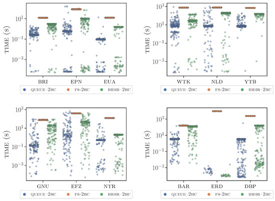
Figure 7.
Running times of fs–2hc, bidir–2hc and queue–2hc on some of the considered inputs. The y-axis is log-scaled to magnify the differences.
Analysis. Our experiments’ main outcomes are essentially two. First and foremost, we observe that queue–2hc worst-case analysis deviates from the performance in practice. In fact, despite the super-cubic worst-case time per update, queue–2hc is always much faster than fs–2hc in our experiments, up to several orders of magnitude faster. Moreover, it is also faster than bidir–2hc, on average. Of particular interest are the improvements observed in weighted instances, where bidir–2hc is not particularly effective and slow enough to be close to fs–2hc (see instances nld or lux). More specifically, queue–2hc achieves superior performance with respect to bidir–2hc update times, up to several orders of magnitude smaller update times (see, e.g., baa or bioinstances). The only exception is graph erd, where the two solutions behave similarly and both exhibit extremely low update times, compared to the time spent by fs–2hc. This might be due to the fact that a small number of operations suffice to update the labeling in this instance (as the graph is quite dense). Hence both solutions are very effective, likely close to an optimal behavior, and the difference is just induced by the determination of the cover graphs. For the sake of fairness, similar behavior is observed in instance ntr, where however queue–2hc is slightly faster.
Thus, on the whole, the performance of queue–2hc is much closer to that of the very efficient resume–2hc for incremental updates [8], which is considered suited to be applied to mine distances from massive time-evolving graphs in real-time contexts [27]. This suggests queue–2hc as well can be considered a reasonable solution for real-time contexts, and that in any case should the preferred option to be adopted in time-evolving scenarios when decremental graph operations must be handled.
5. Conclusions and Future Work
In this paper, we have introduced a new dynamic algorithm, named queue–2hc, to update 2-hop-cover labelings, as a consequence of decremental updates, in time-evolving graphs. We have shown its correctness and analyzed its computational complexity in the worst case. Not surprisingly, the worst-case analysis does not capture well the true performance of the new algorithm. In fact, extensive experimentation we conducted, to assess the performance of queue–2hc, shows queue–2hc is very effective in practice, and outperforms by far the only other known solutions for the problem, i.e., the recomputation from scratch [7] and algorithm bidir–2hc [26]. Therefore, we provide strong evidence that queue–2hc can considered the reference solution to allow distance mining when decremental graph operations can occur in time-evolving scenarios.
To achieve a complete framework for handling efficiently distance queries in massive time-evolving graphs, future works following this study should concentrate on removing the main limitation of the only known algorithm able to handle incremental operations that is resume–2hc [8]. In fact, this algorithm ignores outdated entries that are induced by incremental modifications: this does not affect correctness but leads to degradation in query performance and to the need for periodic reprocessing (see [8,29] for more details).
Another interesting direction should be to extend the experimental evaluation to: (i) consider the greedy ordering of [3]; (ii) include larger inputs or real-world sequences of graph modifications; (iii) investigate the existence of relationships of correlation between graph features (e.g., density, planarity or regularity) and the performance of both 2-hop-cover labelings and the corresponding algorithms, namely fs–2hc, resume–2hc and queue–2hc. This could lead to a more refined analysis explaining why dynamic approaches are so effective in practice, despite bad worst-case bounds (as done in the past for other algorithmic frameworks, such as speed-up techniques for Dijkstra’s algorithm in road networks).
Finally, it would be remarkable to develop an algorithm even faster than queue–2hc, in practice. An idea in this sense could be that of adopting a sort of memorization approach, by precomputing and maintaining, during the evolution of the graph, some additional (compact) data structure storing information about central vertices or critical arcs, to faster identify or update outdated label entries. The benefits of this strategy, however, could be limited due to overhead that would be required to also update the additional data structure itself. An attractive alternative could be to find a lower bound on the computational effort that is necessary to update a 2-hop-cover labeling under decremental operations.
Funding
This work has been partially supported by the Italian National Group for Scientific Computation GNCS-INdAM—Program “Finanziamento Giovani Ricercatori 2019-2020”—Project: “Toward Efficient Mining of Massive Dynamic Graphs: Theory and Applications” and by Project “ASSIOMI—Algorithms, Systems and Devices for Machine Monitoring and Diagnosing in Smart Factories (Algoritmi Sistemi e diSpositivI per mOnitoraggio e diagnostica di Macchine per le fabbriche Intelligenti)”.
Conflicts of Interest
The authors declare no conflict of interest.
References
- Vieira, M.V.; Fonseca, B.M.; Damazio, R.; Golgher, P.B.; Reis, D.C.; Ribeiro-Neto, B.A. Efficient search ranking in social networks. In Proceedings of the 16th ACM Conference on Conference on Information and Knowledge Management (CIKM 2007), Lisbon, Portugal, 6–10 November 2007; pp. 563–572. [Google Scholar]
- Abraham, I.; Delling, D.; Goldberg, A.V.; Werneck, R.F. Hierarchical Hub Labelings for Shortest Paths. In European Symposium on Algorithms; Springer: Berlin/Heidelberg, Germany, 2012; Volume 7501, pp. 24–35. [Google Scholar]
- Delling, D.; Goldberg, A.V.; Pajor, T.; Werneck, R.F. Robust Distance Queries on Massive Networks. In Proceedings of the 22st European Symposium on Algorithms (ESA 2004), Wroclaw, Poland, 8–10 September 2014; Springer: Berlin/Heidelberg, Germany, 2014; Volume 8737, pp. 321–333. [Google Scholar]
- Cionini, A.; D’Angelo, G.; D’Emidio, M.; Frigioni, D.; Giannakopoulou, K.; Paraskevopoulos, A.; Zaroliagis, C. Engineering Graph-Based Models for Dynamic Timetable Information Systems. J. Discret. Algorithms 2017, 46–47, 40–58. [Google Scholar] [CrossRef]
- Bonchi, F. Distance-Based Community Search. In Proceedings of the 45th International Conference on Current Trends in Theory and Practice of Computer Science (SOFSEM), Novy Smokovec, Slovakia, 27–30 January 2019; Catania, B., Královic, R., Nawrocki, J.R., Pighizzini, G., Eds.; Springer: Berlin/Heidelberg, Germany, 2019; Volume 11376, pp. 21–27. [Google Scholar] [CrossRef]
- Wei, H.; Yu, J.X.; Lu, C.; Jin, R. Reachability Querying: An Independent Permutation Labeling Approach. VLDB J. 2018, 27, 1–26. [Google Scholar] [CrossRef]
- Akiba, T.; Iwata, Y.; Yoshida, Y. Fast exact shortest-path distance queries on large networks by pruned landmark labeling. In Proceedings of the International Conference on Management of Data (SIGMOD 2013), New York, NY, USA, 22–27 June 2013; pp. 349–360. [Google Scholar]
- Akiba, T.; Iwata, Y.; Yoshida, Y. Dynamic and historical shortest-path distance queries on large evolving networks by pruned landmark labeling. In Proceedings of the 23rd Int. World Wide Web Conference (WWW 2014), Seoul, Korea, 7–11 April 2014; pp. 237–248. [Google Scholar]
- Cheng, J.; Yu, J.X. On-line exact shortest distance query processing. In Proceedings of the 12th International Conference on Extending Database Technology (EDBT 2009), Saint-Petersburg, Russia, 23–26 March 2009; pp. 481–492. [Google Scholar]
- Jiang, M.; Fu, A.W.C.; Wong, R.C.W. Exact Top-k Nearest Keyword Search in Large Networks. In Proceedings of the 2015 ACM SIGMOD International Conference on Management of Data (SIGMOD 2015), Melbourne, Australia, 31 May–4 June 2015; ACM: New York, NY, USA, 2015; pp. 393–404. [Google Scholar] [CrossRef]
- Borassi, M.; Crescenzi, P.; Habib, M.; Kosters, W.A.; Marino, A.; Takes, F.W. Fast diameter and radius BFS-based computation in (weakly connected) real-world graphs: With an application to the six degrees of separation games. Theor. Comput. Sci. 2015, 586, 59–80. [Google Scholar] [CrossRef]
- Uras, T.; Koenig, S. Subgoal graphs for fast optimal pathfinding. Game AI Pro 2015, 2, 145–159. [Google Scholar]
- D’Emidio, M.; Forlizzi, L.; Frigioni, D.; Leucci, S.; Proietti, G. Hardness, approximability, and fixed-parameter tractability of the clustered shortest-path tree problem. J. Comb. Optim. 2019, 38, 165–184. [Google Scholar] [CrossRef]
- D’Angelo, G.; D’Emidio, M.; Frigioni, D. Fully dynamic update of arc-flags. Networks 2014, 63, 243–259. [Google Scholar] [CrossRef]
- D’Angelo, G.; D’Emidio, M.; Frigioni, D.; Vitale, C. Fully Dynamic Maintenance of Arc-Flags in Road Networks. In Proceedings of the 11th International Symposium on Experimental Algorithms (SEA 2012), Bordeaux, France, 7–9 June 2012; Springer: Berlin/Heidelberg, Germany, 2012; Volume 7276, pp. 135–147. [Google Scholar]
- Bauer, R.; Wagner, D. Batch Dynamic Single-Source Shortest-Path Algorithms: An Experimental Study. In Proceedings of the 8th International Symposium on Experimental Algorithms (SEA 2009), Dortmund, Germany, 4–6 June 2009; Springer: Berlin/Heidelberg, Germany, 2009; Volume 5526, pp. 51–62. [Google Scholar]
- Bast, H.; Delling, D.; Goldberg, A.V.; Müller-Hannemann, M.; Pajor, T.; Sanders, P.; Wagner, D.; Werneck, R.F. Route Planning in Transportation Networks. In Algorithm Engineering; Springer: Cham, Switzerland, 2016; Volume 9220, pp. 19–80. [Google Scholar]
- Cohen, E.; Halperin, E.; Kaplan, H.; Zwick, U. Reachability and Distance Queries via 2-Hop Labels. SIAM J. Comput. 2003, 32, 1338–1355. [Google Scholar] [CrossRef]
- Fu, A.W.C.; Wu, H.; Cheng, J.; Wong, R.C.W. IS-Label: An Independent-set Based Labeling Scheme for Point-to-point Distance Querying. Proc. VLDB 2013 2013, 6, 457–468. [Google Scholar] [CrossRef]
- Jin, R.; Ruan, N.; Xiang, Y.; Lee, V.E. A highway-centric labeling approach for answering distance queries on large sparse graphs. In Proceedings of the International Conference on Management of Data (SIGMOD 2012), Scottsdale, AZ, USA, 20–24 May 2012; pp. 445–456. [Google Scholar]
- Delling, D.; Dibbelt, J.; Pajor, T.; Werneck, R.F. Public Transit Labeling. In Experimental Algorithms; Bampis, E., Ed.; Springer International Publishing: Cham, Switzerland, 2015; pp. 273–285. [Google Scholar]
- Qin, Y.; Sheng, Q.Z.; Zhang, W.E. SIEF: Efficiently Answering Distance Queries for Failure Prone Graphs. In Proceedings of the 18th Int. Conference on Extending Database Technology (EDBT 2015), Brussels, Belgium, 23–27 March 2015; pp. 145–156. [Google Scholar]
- Wei, F. TEDI: Efficient Shortest Path Query Answering on Graphs. In Proceedings of the ACM SIGMOD International Conference on Management of Data (SIGMOD 2010), Indianapolis, IN, USA, 6–11 June 2010; pp. 99–110. [Google Scholar]
- Delling, D.; Goldberg, A.V.; Pajor, T.; Werneck, R.F. Customizable route planning. In Proceedings of the 10th Symposium on Experimental Algorithms (SEA 2011), Kolimpari, Chania, Crete, Greece, 5–7 May 2011; Springer: Berlin/Heidelberg, Germany, 2011; Volume 6630, pp. 376–387. [Google Scholar]
- D’Emidio, M.; Khan, I. Dynamic Public Transit Labeling. In Proceedings of the Computational Science and Its Applications (ICCSA 2019), 19th International Conference, Saint Petersburg, Russia, 1–4 July 2019; Misra, S., Gervasi, O., Murgante, B., Stankova, E.N., Korkhov, V., Torre, C.M., Rocha, A.M.A.C., Taniar, D., Apduhan, B.O., Tarantino, E., Eds.; Proceedings, Part I. Springer: Cham, Switzerland, 2019; Volume 11619, pp. 103–117. [Google Scholar] [CrossRef]
- D’Angelo, G.; D’Emidio, M.; Frigioni, D. Fully Dynamic 2-Hop Cover Labeling. J. Exp. Algorithmics 2019, 24, 1.6:1–1.6:36. [Google Scholar] [CrossRef]
- D’Angelo, G.; D’Emidio, M.; Frigioni, D. Distance Queries in Large-Scale Fully Dynamic Complex Networks. In Proceedings of the 27th International Workshop on Combinatorial Algorithms (IWOCA 2016), Helsinki, Finland, 17–19 August 2016; Springer: Cham, Switzerland, 2016; Volume 9843, pp. 109–121. [Google Scholar]
- Weller, M. Optimal Hub Labeling is NP-complete. arXiv, 2014; arXiv:1407.8373. [Google Scholar]
- Cicerone, S.; D’Emidio, M.; Frigioni, D. On Mining Distances in Large-Scale Dynamic Graphs. In Proceedings of the 19th Italian Conference on Theoretical Computer Science, Urbino, Italy, 18–20 September 2018; Volume 2243, pp. 77–81. [Google Scholar]
- Bergamini, E.; Meyerhenke, H. Fully-dynamic Approximation of Betweenness Centrality. In Algorithms-ESA; Springer: Berlin/Heidelberg, Germany, 2015. [Google Scholar]
- Hayashi, T.; Akiba, T.; Kawarabayashi, K. Fully Dynamic Shortest-Path Distance Query Acceleration on Massive Networks. In Proceedings of the 25th ACM International on Conference on Information and Knowledge Management (CIKM 2016), Indianapolis, IN, USA, 24–28 October 2016; pp. 1533–1542. [Google Scholar]
- D’Andrea, A.; D’Emidio, M.; Frigioni, D.; Leucci, S.; Proietti, G. Experimental Evaluation of Dynamic Shortest Path Tree Algorithms on Homogeneous Batches. In Proceedings of the 13th International Symposium on Experimental Algorithms (SEA 2014), Copenhagen, Denmark, 29 June–1 July 2014; Springer: Cham, Switzerland, 2014; Volume 8504, pp. 283–294. [Google Scholar]
- Henzinger, M.; Krinninger, S.; Nanongkai, D. Decremental Single-Source Shortest Paths on Undirected Graphs in Near-Linear Total Update Time. J. ACM 2018, 65. [Google Scholar] [CrossRef]
- Chuzhoy, J.; Khanna, S. A New Algorithm for Decremental Single-Source Shortest Paths with Applications to Vertex-Capacitated Flow and Cut Problems. In Proceedings of the 51st Annual ACM SIGACT Symposium on Theory of Computing, Phoenix, AZ, USA, 26 June 2019; Association for Computing Machinery: New York, NY, USA, 2019; pp. 389–400. [Google Scholar] [CrossRef]
- Staudt, C.L.; Sazonovs, A.; Meyerhenke, H. NetworKit: A tool suite for large-scale complex network analysis. Netw. Sci. 2016, 4, 508–530. [Google Scholar] [CrossRef]
- Delling, D.; Goldberg, A.V.; Savchenko, R.; Werneck, R.F. Hub Labels: Theory and Practice. In Proceedings of the 13th Symposium on Experimental Algorithms (SEA 2014), Copenhagen, Denmark, 29 June–1 July 2014; Springer: Cham, Switzerland, 2014; Volume 8504, pp. 259–270. [Google Scholar]
- Leskovec, J.; Krevl, A. SNAP Datasets: Stanford Large Network Dataset Collection. 2014. Available online: http://snap.stanford.edu/data (accessed on 11 February 2020).
- Rossi, R.A.; Ahmed, N.K. The Network Data Repository with Interactive Graph Analytics and Visualization. In Proceedings of the 29th AAAI Conference on Artificial Intelligence (AAAI 2015), Austin, TX, USA, 25–30 January 2015. [Google Scholar]
- Kunegis, J. KONECT: The Koblenz Network Collection. 2013. Available online: http://konect.uni-koblenz.de/ (accessed on 11 February 2020).
- Bollobás, B. Random Graphs; Cambridge University Press: Cambridge, UK, 2001. [Google Scholar]
- Albert, R.; Barabási, A.L. Statistical mechanics of complex network. Rev. Mod. Phys. 2002, 74, 47–97. [Google Scholar] [CrossRef]
- D’Andrea, A.; D’Emidio, M.; Frigioni, D.; Leucci, S.; Proietti, G. Dynamic Maintenance of a Shortest-Path Tree on Homogeneous Batches of Updates: New Algorithms and Experiments. ACM J. Exp. Algorithmics 2015, 20, 1.5:1.1–1.5:1.33. [Google Scholar] [CrossRef]
- Jamour, F.; Skiadopoulos, S.; Kalnis, P. Parallel Algorithm for Incremental Betweenness Centrality on Large Graphs. IEEE Trans. Parallel Distrib. Syst. 2018, 29, 659–672. [Google Scholar] [CrossRef]


© 2020 by the author. Licensee MDPI, Basel, Switzerland. This article is an open access article distributed under the terms and conditions of the Creative Commons Attribution (CC BY) license (http://creativecommons.org/licenses/by/4.0/).