Abstract
In pulse waveform classification, the convolution neural network (CNN) shows excellent performance. However, due to its numerous parameters and intensive computation, it is challenging to deploy a CNN model to low-power devices. To solve this problem, we implement a CNN accelerator based on a field-programmable gate array (FPGA), which can accurately and quickly infer the waveform category. By designing the structure of CNN, we significantly reduce its parameters on the premise of high accuracy. Then the CNN is realized on FPGA and optimized by a variety of memory access optimization methods. Experimental results show that our customized CNN has high accuracy and fewer parameters, and the accelerator costs only 0.714 W under a working frequency of 100 MHz, which proves that our proposed solution is feasible. Furthermore, the accelerator classifies the pulse waveform in real time, which could help doctors make the diagnosis.
1. Introduction
Pulse diagnosis is a non-invasive diagnostic method, and pulse wave has been proved to be beneficial to the diagnosis of cardiovascular diseases [1,2,3,4,5]. In traditional Chinese medicine (TCM), doctors distinguish different pulse types according to a variety of parameters, including pulse waveform, depth, width, length, and frequency, then make the corresponding diagnosis [6]. Among these properties, pulse waveform is the most critical factor in classifying the pulse types, which is an essential task of pulse diagnosis devices. Therefore, researchers have widely studied pulse waveform classification in recent years [1,3,4,7,8,9,10,11,12,13].
According to [6], pulse waveforms can be divided into four basic types: Ping, Xian, Hua, and Se separately, shown in Figure 1. These four waveforms are the commonest types with typical features: Ping pulse has two maximum points, one minimum point, and one inflection point; Xian pulse has a broader peak than Ping pulse, two maximum points, and 1 or 0 inflection points; Hua pulse has two maximum points, one minimum point, and no inflection point; Se pulse has only one clear maximum point.
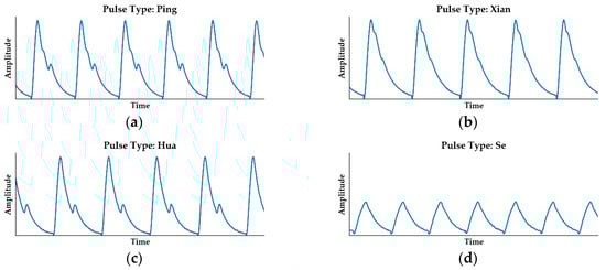
Figure 1.
Four typical types of pulse waveforms. (a) Ping pulse; (b) Xian pulse; (c) Hua pulse; (d) Se pulse.
Pulse wave processing includes three steps [7]: data collection and preprocessing, feature extraction, and classification. During preprocessing, to improve the signal-noise ratio (SNR) and obtain a higher quality of the signal, the digital filters are designed to eliminate power-line interference and remove the baseline shift.
Researchers have developed several feature extraction approaches, including the time-domain methods, frequency-domain methods [14], and nonlinear analysis methods. In time-domain methods [15,16], the threshold method has low complexity and is easy to realize; however, the usually fixed threshold leads to its poor robustness. The disadvantages of the model fitting method [12] are that it has high computational complexity, and the details of the original pulse wave are neglected. In frequency-domain methods, the power spectrum analysis [14] and cepstral analysis are two conventional methods; however, the extracted feature parameters’ significances are non-intuitive and difficult to explain. Moreover, time-frequency analysis methods, including short-time Fourier transform and wavelet transform [17,18,19], also are complex in computation and hard to employ.
In classification, machine learning and deep learning methods based on statistical recognition, including support vector machine (SVM) [20], decision tree [21], and deep neural network, have also been widely studied. Hu et al. [7] reported the convolutional neural network (CNN) classification, and its accuracy is higher compared to other classification algorithms.
However, CNN’s training and inference process require plenty of computations, which demand high computing power equipment, such as a graphics processing unit (GPU) or large servers [22]. They usually consume much power and cannot be integrated into a portable device. Field-programmable gate array (FPGA) is an ideal platform to address this problem. After importing the trained model parameters from GPU, we can use FPGA to conclude and obtain the classification results of the input pulse wave.
Many researchers have implemented CNN on FPGA, and optimization methods have been widely studied [22,23,24,25,26,27,28,29,30,31]. The solutions can be divided into three categories: computational kernel optimization, bandwidth optimization, and optimization of CNN models. Memory access reduction [24], which minimizes data movement, has been employed to increase throughput. Data quantization [22,26,28,30], which is usually used on FPGA, helps increase parallelism and accelerate the computation speed. In particular, binarized neural network (BNN) [32] can drastically reduce the memory size and transform multiply-accumulate operation (MAC) into bitwise operation.
In this paper, we propose an FPGA-based CNN accelerator for pulse waveform classification. First, we employ a micro-electro-mechanical-system (MEMS) sensor array to collect the pulse wave signal and designed digital filters to obtain a clearer signal. Moreover, CNN is selected to classify the different types of pulse waveforms. Moreover, to reduce CNN’s parameters and the required buffer size, we specially design a CNN model according to a set of experiments. Finally, we optimize the hardware design using three memory access optimization methods and realize the accelerator, which consumes less power and has low latency.
The rest of this paper is organized as follows. Section 2 describes the system design flow: data collection and preprocessing, the background of CNNs, and hardware design architecture. Section 3 explains the network model design and parameter reduction, three optimization methods, the corresponding result, and the comparison with previous studies. Section 4 concludes this paper.
2. System Design
2.1. System Design Flow
The system design flow is shown in Figure 2. First, a MEMS pressure sensor array is used to acquire the pulse wave of subjects. Then we preprocess the collected data by a series of digital filters to obtain clearer signals and build a dataset. Secondly, a CNN model is trained on the dataset and modified iteratively to reduce the memory footprint and the number of parameters. Thirdly, the hardware design defines the accelerator’s architecture according to the software algorithm, divides the functional modules reasonably, and realizes the register-transfer-level (RTL) circuit by Verilog code.
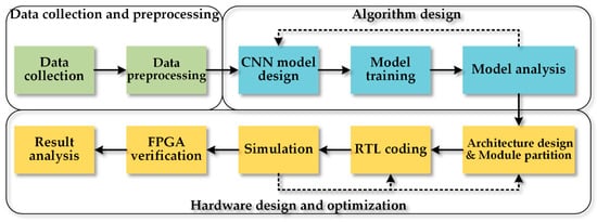
Figure 2.
The system design flow includes data collection and preprocessing, algorithm design, and hardware design and optimization.
According to the simulation results, the RTL design also needs to be updated iteratively to satisfy the design specifications. Eventually, the hardware design will be implemented on the FPGA board. The design’s function and performance are evaluated in real practice, and the result is further analyzed.
2.2. Data Collection and Preprocessing
In our previous work [33], a pulse signal acquisition system was designed to collect the wrist pulse waves. MEMS sensor is employed to transforms the pressure signal into a voltage signal, and an array composed of 12 such sensors outputs 12 differential signals. Operational amplifiers magnify the signals, which are polled by a multiplexer (MUX). Then the MUX’s output signal is sampled by an analog-digital converter (ADC), transformed into a digital signal, transmitted to PC, and stored into the disk. The sampling frequency for each channel signal is 218 Hz, much higher than the pulse signal.
After collecting the subjects’ original pulse waves, we need to preprocess them and standardize the data. The complete data preprocessing flow is shown in Figure 3. To classify and label the waveforms more accurately, we design digital filters to obtain a clearer signal. First, we roughly select a two-minute segment from the raw pulse signal, then filter the selected segment by a low-pass filter (LPF, the cut-off frequency is 40 Hz) to remove the power-line interference. Second, to remove the baseline wander, we use a high-pass filter (HPF, the cut-off frequency is 0.2 Hz) to filter the output of LPF. Then we select a certain length of the segment from the prior result to keep the length of all data consistent. Third, the corresponding segment of the original pulse wave is normalized, labeled manually, and stored in the dataset. Eventually, the dataset, whose size is 2829, includes 1106 Ping pulse, 853 Hua pulse, 376 Xian pulse, and 494 Se pulse.
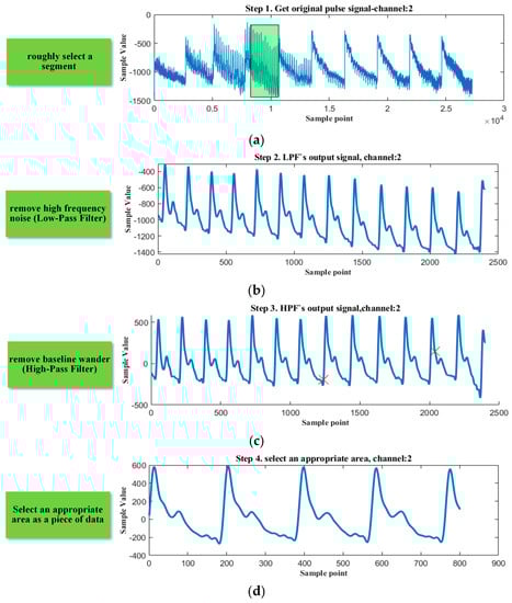
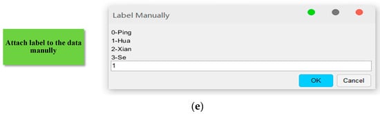
Figure 3.
Data collection and preprocessing. (a) roughly select a segment; (b) remove high frequency noise; (c) remove baseline wander; (d) select an appropriate area as a piece of data; (e) normalize, label, and store the data.
2.3. Algorithm Design: Structure of CNN
The pulse signal belongs to the time-series signal so that the pulse waveform classification will deal with the 1-dimension signal. Recurrent neural network (RNN) and long-short term memory (LSTM) are usually used to predict the next moment’s output according to a prior time-series signal. However, their performances are not better than the convolution neural network (CNN) when it refers to classification because they concern more about the relationship in the context, not the overall feature. Therefore, we select CNN as the classification method.
Figure 4a shows a CNN model, which contains two types of layers, the convolution (CONV) layers, and the fully connected (FC) layers. CONV layer refers to 3 operation types: convolution, activation, and pooling separately, as shown in Figure 4b. The input tensor has channels of features, and the length of each channel is . The CONV layer’s computational procedures for an output channel are shown in Figure 4c. For each output channel , each input channel is processed by a corresponding sliding window, which is also named convolution kernel. Then the convolution results of input channels are accumulated, processed by a rectified linear unit (ReLU), then pooled by a maximum function. After the CONV layers, the feature maps are flattened to a 1-D tensor, which is the input tensor of the FC layer. The FC layer’s computational function is
here y is the output tensor, a column vector of length n, x is the input tensor, a column vector of length m, W is a matrix of weights, whose size is , b is a column vector of bias, whose length is n.
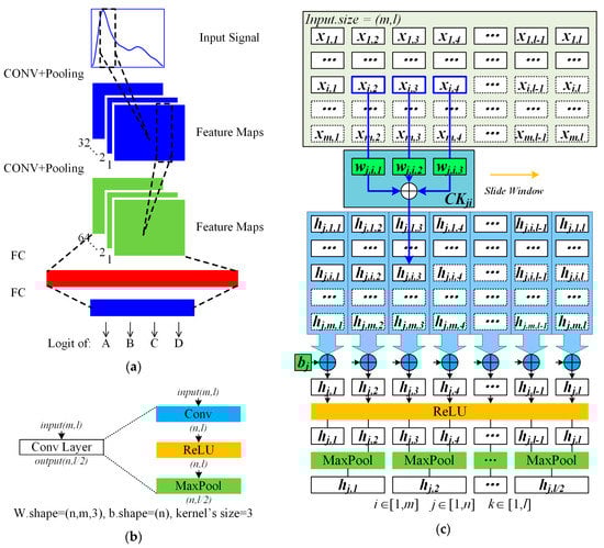
Figure 4.
CNN model and convolution (CONV) layer. (a) a CNN model includes 2 CONV layers and 2 FC layers; (b) 3 operation types of CONV layer; (c) complete calculation procedures of convolution layer.
For the algorithm design of software, the confusion matrix is usually used to evaluate the model, and accuracy is one of the most critical indexes of the CNN model. The definition of a confusion matrix is: true positive (TP) means the number of positive data classified correctly, true negative (TN) means the number of negative data classified correctly, false positive (FP) means the number of negative data classified incorrectly, and false negative (FN) means the number of positive data classified incorrectly. The accuracy, precision, sensitivity, F1 score and macro F1 are calculated by:
However, in the actual deployment on FPGA, the limited FPGA resource, especially Block RAM (BRAM), will restrict the number of model parameters, especially weights of the CONV and FC layers. Therefore, we optimize the CNN model by adjusting its number of layers and structure to reduce the parameters.
2.4. Hardware System Design
According to the above analysis, the software computation procedure of CONV layer is shown in Algorithm 1.
| Algorithm 1. Algorithm of CONV layer. |
| for j in range(n): # loop 1 for i in range(m): # loop 1.1 load input[i][:]; load weights[j][i][3]; conv_out[j][i][:] = CONV(input[i][:], weights[j][i]); store conv_out[j][i][:]; for j in range(n): # loop 2 for k in range(l): # loop 2.1 load conv_out[j][:][k]; accu_out[j][k] = ACCU(conv_out[j][:][k]); accu_out[j][k] += bias[j] for j in range(n): # loop 3 for k in range(l): # loop 3.1 relu_out[j][k] = accu_out[j][k]>0 ? accu_out[j][k]:0; for k in range(l/2): # loop 3.1 maxp_out[j][k] = max(relu_out[j][2*k], relu_out[j][2*k+1]); |
Because the iteration variables of loop 2, loop 3, and loop 4 are the same, we can merge the three loops into a loop, which executes the accumulation, ReLU, and MaxPooling (ARMP) successively. The core idea of the accelerator is loop unrolling. To accelerate the computation process, we can use multiple convolution kernel (CK) modules and ARMP modules to calculate in parallel.
2.4.1. System Architecture Design
In the hardware system, the accelerator is composed of three parts: the computation modules, the control modules, and the memory modules. The system architecture is shown in Figure 5. According to the description in Section 2.3, a CONV layer has three operation modules: CK and accumulator, ReLU, and maximum pooling. Owing to the substantial data dependence between the accumulator’s input and the convolution kernel’s output, we divide the two operations. We use CK modules to realize the convolution procedure and ARMP modules to process the rest computation part of the convolution layer. Moreover, we perform the FC layer using a FC module. The entire system has eight CK modules, four ARMP modules, and one FC module, which are all pipelined to accelerate the arithmetic speed.
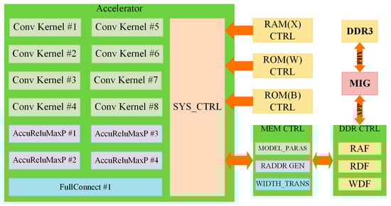
Figure 5.
CNN accelerator system architecture includes 3 types of computation module, system controller (SYS_CTRL), memory controller (MEM_CTRL), and Double-Data-Rate SDRAM controller (DDR_CTRL). The red arrows mean the direction of data flow.
The other facet of the system design is memory modules. The input signal is preloaded into a Block RAM by a microcontroller. The trained weights and biases are programmed into two read-only memory (ROM), respectively. As the output tensor of the CK module needs to be cached, and its size is too large to be stored on the FPGA chip, we use Double-Data-Rate SDRAM (DDR) to cache the intermediate results. Because read and write operations are simultaneous, the data stream needs to be cached, we use three asynchronous First-In-First-Out (FIFO) to serve as the data buffers: a read address FIFO (RAF) as a read address buffer, a read data FIFO (RDF) as a read data buffer, and a write data FIFO (WDF) as write data buffer.
The controller modules consist of system controller (SYS_CTRL), memory controller (MEM_CTRL), and DDR controller (DDR_CTRL). SYS_CTRL controls the work state of CNN, emit memory access request signal according to the current computation type. In addition, MEM_CTRL generates the read address and convert the width of data according to the request type and the current layer. DDR_CTRL controls the work state of the three FIFOs.
2.4.2. Computation Modules Design
The CK module is the computation-intense part of the system, which is pipelined to advance the operation speed. In the CNN software algorithm, we need to pad 0 before and after the input tensor. The RTL circuit design is shown in Figure 6. Only when the valid signal of input is high, will the input be selected as the value to participate in the calculation. While detecting the valid signal’s negative edge, the value 0, not the input will be transmitted into reg_din.
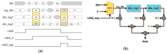
Figure 6.
Convolution kernel (CK) design. (a) CK’s timing diagram. (b) CK’s (Register-Transfer-Level) RTL circuit design.
In the ARMP module, an accumulator is employed to execute the accumulation. Similar to the previous treatment, when detecting the negative edge of input’s valid signal, it is the bias, not the input transmitted into reg_din. The ReLU is implemented by judging the sign bit of the data. Furthermore, the MaxPooling is realized by a comparator.
In FC module, a multiplier and an accumulator are used to realize the formula (1). Unlike the above two calculations, the FC module has a timing requirement that the input data and weights must be transferred synchronously.
2.4.3. Control Modules Design
The controller design is mainly based on the finite state machine (FSM). When the start signal is triggered, the FSM begins to calculate. The input of the first CONV layer, which is marked as CONV1, is from a random-access memory (marked as RAMX), while the inputs of other CONV layers are from DDR. The principle of the SYS_CTRL module is shown in Figure 7a. The system first runs the convolution step of CONV1, performs its ARMP operation, and executes CONV and ARMP layer by layer. When all convolution layers are handled thoroughly, the SYS_CTRL starts to calculate the FC layers. Finally, output the result when FC layers are finished.
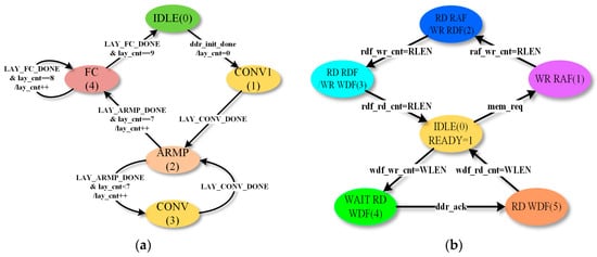
Figure 7.
Control modules design. (a) State transition diagram of System controller (SYS_CTRL) module. (b) State transition diagram of DDR controller (DDR_CTRL) module.
DDR_CTRL module controls 3 FIFOs: read address FIFO (RAF), read data FIFO (RDF), and write data FIFO (WDF). The state transition diagram is shown in Figure 7b. When memory access request signal mem_req is valid, DDR_CTRL will be transmitted into WR_RAF: Read addresses transferred by MEM_CTRL are accepted and stored. When all read addresses are transferred, DDR_CTRL starts to read the RAF and emit read request signal to Memory Interface Generator (MIG). When the RDF receives a certain length of the request, the data will be transferred to SYS_CTRL to feed the computation modules. The output of computation modules is written into WDF, and until it reaches a certain length, DDR_CTRL requests MIG to write it in burst mode.
3. Optimization Methods and Results
3.1. Network Model Design and Parameter Reduction
According to our analysis, the main part of weight parameters is from the first FC layer in the CNN model. We employ three methods to reduce the parameters’ number:
- Downsampling the data. We can use downsampling to reduce the amount of computation significantly while the accuracy of classification remains high.
- Use more CONV layers to reduce the FC layer’s weights. The more CONV layers, the shorter length of the FC layer’s input tensor, and the fewer FC layer’s parameters.
- Modify the CONV layers’ structure to reduce CONV layers’ parameters. Reducing the ratio of output channels to input channels can effectively reduce the parameters of the convolution layers.
To design a CNN model that has higher accuracy and fewer parameters, we conduct several experiments based on our development environment, which includes PyTorch 1.4.0 (CUDA version), Python 3.6.5, and a GPU of NVIDIA GTX 965M. The corresponding model parameters include the number of CONV layers, the ratio of output channels to input channels, and the input tensor’s length. When the number of CONV layers is 2, 3, 4, 5, 6, 7, and 8, its influence on the CNN model is shown in Figure 8a. As the number of convolution layers increases, the number of weight parameters decreases, and the accuracy increases accordingly. When the number of CONV layers is greater than 5, the increase in it has no significant effect on the accuracy, and the speed of parameter reduction also decreases.
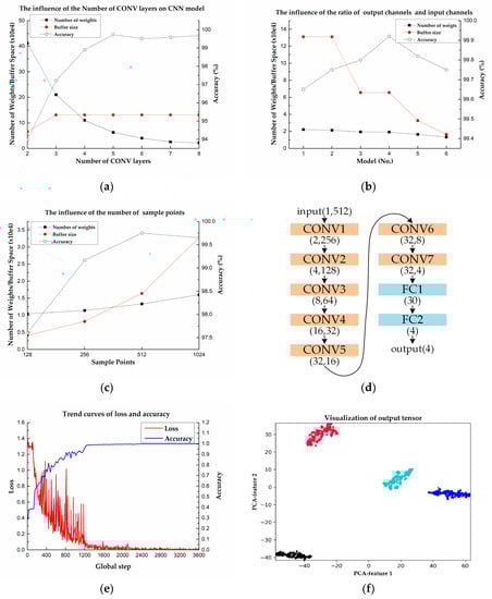
Figure 8.
CNN network model design and parameter reduction. (a) The effects of the number of CONV layers on CNN model. (b) The effects of the ratio of output channels and input channels. (c) The effects of the number of sample points of input tensor. (d) The CNN model which has relative high accuracy, less required buffer size, and a few parameters. (e) The trend curves of loss and accuracy during training. (f) Visualization of FC1’s output tensor.
To reduce the required buffer size, we modify the CNN’s structure by changing the ratio of output channels and input channels of CONV layers. We design six models with 7 CONV layers and 2 FC layers, while their structures are different, as shown in Table 1. In the models, layer 7 has 32 output tensors, whose size is 4. They are flattened into a tensor with a length of 128, which serves as the input features of layer 8. The result is shown in Figure 8b, demonstrating that the model with a lower ratio needs fewer required buffer size while maintaining high accuracy.

Table 1.
Different structures of 6 CNN models.
Moreover, to reduce the computation amount, we take the downsampling of the original signal, which has a length of 1024 sample points and get the signals with a length of 512, 256, 128, respectively. The corresponding sampling frequency is 109.00 Hz, 54.50 Hz, 27.25 Hz separately, which will not result in signals with alias frequencies according to Nyquist’s theorem. As shown in Figure 8c, the results indicate that the accuracy is reduced when the input signal’s length is fewer than 512. Based on the above experiments, the final CNN, which has 12,150 parameters in total, is shown in Figure 8d.
Because the amount of data is relatively small, we use 5-fold cross-validation to estimate the generalization error and ensure the model’s effectiveness. For each of the 5 folds, each model is trained for 300 epochs using the adaptive moment estimation (ADAM) optimizer and the cross-entropy loss function. The learning rate with an initial value of 0.003 decreases 10 times every 100 epochs, and the batch size is 200. The training process is shown in Figure 8e, which indicates that the loss function decreases, and the accuracy increases gradually.
The average of the classification results of 5 models is used as the estimation of CNN’s performance. Moreover, to avoid the error introduced by the random extraction of the folds, we repeated the experiment 10 times. The mean accuracy is 99.27% and the standard deviation is 0.19%, which illustrates the CNN model has excellent generalization performance. The mean value of macro F1, which is calculated by using formula (3)–(6), is 98.75% and the standard deviation is 0.32%, which indicates the model has a highly stable classification ability for 4 types of waveforms.
Hu et al. designed a CNN model with three convolution layers and two FC layers [7]. Under the same experimental setup, we tested the design on our dataset, and the average classification accuracy is 99.47%, which is slightly higher when compared to our model; however, the number of the CNN model’s parameters is 731,214, far more than that of our model, which means it is difficult to realize on FPGA. The results illustrate that we substantially reduced the scale of the model at the cost of a small reduction of accuracy.
To further check the evaluation result’s correctness, we employ principal component analysis (PCA) to realize FC1’s output tensor’s visualization, which is shown in Figure 8f. It shows that most of the data can be recognized and classified correctly and hence, the model is suitable for the classification of the pulse waveform.
3.2. Hardware System Optimization
3.2.1. Memory Access Optimization Method 1: Continuous Read Mode
The CONV operation’s output is written to DDR in burst mode, so the write addresses are continuous, as Figure 9a shows. However, the input sequence of the ARMP module is different from the output sequence of the CONV module. The read addresses are random, which is shown in Figure 9b. Figure 9c provides the principle of a usual solution. The read address of 29 bits is divided into two parts: the part of bit 2 to bit 0 is the data mask to select the valid word in the 256 bits which are read back from DDR, and the other part of bit 28 to bit 3 is the aligned address which MIG operates. The timing diagram of the solution is shown in Figure 9d. However, the time to read back from DDR is far longer than the necessary time to consume, which leads to low data throughput and poor efficiency.
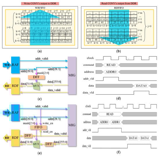
Figure 9.
Memory access module design and optimization. (a) Write CONV’s output to DDR. (b) Read CONV’s output from DDR. (c) Usual solution to discrete read address. (d) Timing diagram of usual solution to discrete read address. (e) Optimized solution to discrete read address. (f) Timing diagram of optimized solution to discrete read address.
To advance memory access speed, we design an optimized memory access solution, which is shown in Figure 9e. We employ a FIFO to buffer the data mask to nonstop transfer the aligned address to MIG and achieve a continuous read operation. The data which is read back is deposited in a D Flip-Flop (DFF) to keep the same time latency with signal data_valid. Then the valid word is chosen by the data mask and written into RDF. The timing diagram of the optimized solution is shown in Figure 9f. The optimized solution realizes continuous read and needs to wait MIG read back for only one time, saving plenty of time.
3.2.2. Memory Access Optimization Method 2: Task Pipelining
To further improve the performance of the accelerator, we analyze the memory access mechanism. According to the description in Section 2.4.3, the operation procedures of memory access are writing RAF (marked as task 1), reading RAF and writing RDF (marked as task 2), reading RDF and writing WDF (marked as task 3), and writing DDR (marked as task 4) eventually. The scheme is shown in Figure 10, where the arrows mean the data stream’s flow direction. However, the interval between two adjacent data streams cannot be neglected, which adds unnecessary latency in the whole process.
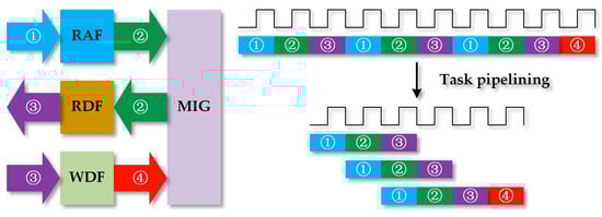
Figure 10.
Task pipelining reduces the interval between tasks.
To reduce the interval, we reschedule the process using the task pipeline, as shown in Figure 10. The FSM described in Figure 8b is divided into four independent FSMs. Therefore, tasks 1, 2, and 3 can run in parallel without interference and the latency of a complete memory access process is reduced remarkably.
3.2.3. Memory Access Optimization Method 3: Use BRAM
The external memory DDR provides a lot of extra cache space for user logic, which allows us to accelerate more complex algorithms. Nevertheless, because it has only a single port and cannot read and write simultaneously, it needs FIFOs as the data buffers, and complex control logic is added. Also, the throughput of DDR is limited by clock frequency, causing a lot of time consumption. Plus, many ports between FPGA and DDR can also lead to high power consumption.
Using BRAM integrated into the FPGA chip will address the problems. We can employ two BRAM blocks (marked as RAMA and RAMB), to form the ping-pong structure to improve the throughput of memory access. The optimized system architecture is shown in Figure 11. When the request type is CONV, which means SYS_CTRL will perform CONV computation, the system will read RAMA and write RAMB. When the request type is ARMP, which means SYS_CTRL will perform ARMP computation, it will read RAMB and write RAMA. The ping-pong structure needs no more FIFOs to serve as data buffers because the two BRAM blocks can handle a read or write operation in a clock period.
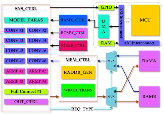
Figure 11.
Optimized system architecture. Two blocks of BRAM which form the ping-pong structure simplify the memory access process and reduce unnecessary latency.
3.2.4. Memory Access Optimization Results
We implement the CNN accelerator on Xilinx FPGA. The device part is Xilinx xc7a100tfgg484-2 (Xilinx, San Jose, CA, USA), and the synthesis tool is Vivado 2018.03 (Xilinx, San Jose, CA, USA). The comparison of the unoptimized solution (marked as Solution 1) and three other optimized solutions is shown in Table 2, which lists each layer’s time consumption. Here the solutions described in Section 3.2.1, Section 3.2.2, and Section 3.2.3 are marked as Solution 2, Solution 3, and Solution 4. As shown in Table 2, the intervals of random read operations take plenty of time, reducing the throughput of memory access. Moreover, the system architecture, which uses the ping-pong structure has higher throughput. The result shows that the time consumed by Solution 4 is significantly reduced by up to 96.8% compared with the unoptimized solution.
Table 2.
Performance of unoptimized and optimized memory access solutions.
The comparison in resource consumption and performance of four solutions on FPGA is shown in Table 3. The result shows that Solution 4, which consumes fewer resources but performs better than Solution 3. Moreover, the power consumed is only 0.714 W under a working frequency of 100 MHz, which is far lower than the system architecture with DDR as cache memory. Moreover, when the system works under a working frequency of 170 MHz, the power consumption is only about 1.089 W, and the latency is 0.487 ms, which also satisfies the real-time requirement.
Table 3.
Resource consumption and performance of different solutions on FPGA.
3.3. Comparison with Related Studies
We compared the proposed design with the state-of-the-art CNN FPGA accelerator designs listed in Table 4. The work in [27], which used the FPGA platform Vertix-7 VX690T (San Jose, CA, USA), realized the AlexNet and occupies more resources. Guo et al. [30] realized the VGG16, which employed Zynq XC7Z020 (San Jose, CA, USA). Moreover, the kind of Zynq FPGA collaborating with an external MCU would consume more power. Geng et al. [31] achieved a low latency compared with [30]; however, the power consumption was still high. Li et al. [26] achieved the AP2D-Net (San Jose, CA, USA) on Ultra96, and the power was pretty low. In our design, the accelerator with a latency of 0.827ms costs only 0.714 W under a working frequency of 100 MHz. Although our CNN model is much simpler, compared to the above designs, the latency and the power of our design are far lower, which meets the requirements of real time and low power.
Table 4.
Comparison with previous FPGA-based CNN implementations.
4. Conclusions
In this paper, we propose an FPGA-based CNN accelerator for pulse waveform classification. First, we employ CNN to classify the different types of pulse waveforms. Moreover, to reduce the number of parameters and the memory used to cache intermediate results, we specially design a CNN model in accordance with experiments, which illustrates that the optimization of the CNN software algorithm has a significant effect on memory reduction. Finally, we implement the CNN algorithm on FPGA, optimize the hardware design by three optimization methods, and realize the accelerator, which costs only 0.714 W under a working frequency of 100 MHz. The hardware optimization dramatically improves the clock speed and reduces memory access latency.
In summary, the specified CNN model and the custom RTL design help reduce resource usage, latency, and power consumption. The software and hardware co-design method helps improve the performance of the accelerator significantly. The low-power and real-time features allow the CNN classification accelerator of pulse waveform to be integrated into the portable devices, and it will play an essential role in doctor diagnosis. In future work, we will further optimize and improve the accelerator’s throughput by employing the data quantization method and other state-of-the-art strategies.
Author Contributions
Conceptualization, C.C. and Y.Z.; Data curation, C.C. and J.H.; Formal analysis, C.C. and J.H.; Funding acquisition, Z.L. and H.Z.; Investigation, C.C.; Methodology, C.C. and Z.L.; Project administration, Z.L. and H.Z.; Resources, Z.L. and Y.Z.; Software, C.C.; Supervision, C.C.; Validation, C.C., S.Z. and J.H.; Visualization, S.Z. and H.Z.; Writing–original draft, C.C.; Writing–review and editing, C.C., Z.L. and H.Z. All authors have read and agreed to the published version of the manuscript.
Funding
This research was funded by the National Major Science and Technology Project (No. 2018ZX01031-201, 2018ZX09201011).
Conflicts of Interest
The authors declare no conflict of interest.
References
- Wang, N.; Yu, Y.; Huang, D.; Xu, B.; Liu, J.; Li, T.; Xue, L.; Shan, Z.; Chen, Y.; Wang, J. Pulse diagnosis signals analysis of fatty liver disease and cirrhosis patients by using machine learning. Sci. World J. 2015, 2015. [Google Scholar] [CrossRef] [PubMed]
- Charbonnier, S.; Galichet, S.; Mauris, G.; Siché, J.P. Statistical and fuzzy models of ambulatory systolic blood pressure for hypertension diagnosis. IEEE Trans. Instrum. Meas. 2000, 49, 998–1003. [Google Scholar] [CrossRef]
- He, D.; Wang, L.; Fan, X.; Yao, Y.; Geng, N.; Sun, Y.; Xu, L.; Qian, W. A new mathematical model of wrist pulse waveforms characterizes patients with cardiovascular disease—A pilot study. Med. Eng. Phys. 2017, 48, 142–149. [Google Scholar] [CrossRef] [PubMed]
- Gomes Ribeiro Moura, N.; Sá Ferreira, A. Pulse waveform analysis of chinese pulse images and its association with disability in hypertension. JAMS J. Acupunct. Meridian Stud. 2016, 9, 93–98. [Google Scholar] [CrossRef] [PubMed]
- Zhang, Z.; Zhang, Y.; Yao, L.; Song, H.; Kos, A. A sensor-based wrist pulse signal processing and lung cancer recognition. J. Biomed. Inform. 2018, 79, 107–116. [Google Scholar] [CrossRef] [PubMed]
- Fei, Z. Contemporary Sphygmology in Traditional Chinese Medicine; People’s Medical Publishing House: Beijing, China, 2003. [Google Scholar]
- Hu, X.; Zhu, H.; Xu, J.; Xu, D.; Dong, J. Wrist pulse signals analysis based on Deep Convolutional Neural Networks. In Proceedings of the 2014 IEEE Conference on Computational Intelligence in Bioinformatics and Computational Biology (CIBCB 2014), Honolulu, HI, USA, 21–24 May 2014. [Google Scholar] [CrossRef]
- Wang, Y.-Y.L.; Hsu, T.-L.; Jan, M.-Y.; Wang, W.-K. Theory and applications of the harmonic analysis of arterial pressure pulse wave. J. Med. Biol. Eng. 2010, 30, 125–131. [Google Scholar] [CrossRef]
- Lu, G.; Jiang, Z.; Ye, L.; Huang, Y. Pulse feature extraction based on improved gaussian model. In Proceedings of the Proceedings—2014 International Conference on Medical Biometrics, ICMB 2014, Shenzhen, China, 30 May–1 June 2014; pp. 90–94. [Google Scholar]
- Tang, A.C.Y.; Chung, J.W.Y.; Wong, T.K.S. Digitalizing traditional chinese medicine pulse diagnosis with artificial neural network. Telemed. e-Health 2012, 18, 446–453. [Google Scholar] [CrossRef] [PubMed]
- Xu, L.S.; Meng, M.Q.H.; Wang, K.Q. Pulse image recognition using fuzzy neural network. In Proceedings of the Annual International Conference of the IEEE Engineering in Medicine and Biology Society, Lyon, France, 22–26 August 2007; Volume 36, pp. 3148–3151. [Google Scholar] [CrossRef]
- Chen, Y.; Zhang, L.; Zhang, D.; Zhang, D. Wrist pulse signal diagnosis using modified Gaussian models and Fuzzy C-Means classification. Med. Eng. Phys. 2009, 31, 1283–1289. [Google Scholar] [CrossRef] [PubMed]
- Shu, J.J.; Sun, Y. Developing classification indices for Chinese pulse diagnosis. Complement. Ther. Med. 2007, 15, 190–198. [Google Scholar] [CrossRef] [PubMed]
- Liu, Y.H.; Yang, Q.H.; Shi, H.F. Pulse feature analysis and extraction based on pulse mechanism analysis. In Proceedings of the 2009 WRI World Congress on Computer Science and Information Engineering, CSIE 2009, Los Angeles, CA, USA, 31 March–2 April 2009; Volume 7, pp. 53–56. [Google Scholar] [CrossRef]
- Hudoba, G. Vascular health diagnosis by pulse wave analysis. In Proceedings of the SAMI 2010—8th International Symposium on Applied Machine Intelligence and Informatics, Herlany, Slovakia, 28–30 January 2010; pp. 89–91. [Google Scholar] [CrossRef]
- Sareen, M.; Abhinav, A.; Prakash, P.; Anand, S. Wavelet decomposition and feature extraction from pulse signals of the radial artery. In Proceedings of the 2008 International Conference on Advanced Computer Theory and Engineering, Phuket, Thailand, 20–22 December 2008; pp. 551–555. [Google Scholar] [CrossRef]
- Zhang, P.Y.; Wang, H.Y. A framework for automatic time-domain characteristic parameters extraction of human pulse signals. EURASIP J. Adv. Signal Process. 2008, 2008. [Google Scholar] [CrossRef]
- Joshi, A.; Chandran, S.; Jayaraman, V.K.; Kulkarni, B.D. Arterial pulse system modern methods for traditional indian. In Proceedings of the 2007 Annual International Conference of the IEEE Engineering in Medicine and Biology Society, Lyon, France, 22–26 August 2007; pp. 608–611. [Google Scholar] [CrossRef]
- Li, J.; Cao, Y.; Liu, Q.; Jiao, Q. Determination of urinary L-citrulline by enzymatic method. Chin. J. Anal. Chem. 2006, 34, 379–381. [Google Scholar] [CrossRef]
- Wang, K.; Wang, L.; Wang, D.; Xu, L. SVM classification for discriminating cardiovascular disease patients from non-cardiovascular disease controls using pulse waveform variability analysis. Lect. Notes Comput. Sci. 2005, 109–119. [Google Scholar] [CrossRef]
- Wang, H.; Cheng, Y. A quantitative system for pulse diagnosis in traditional Chinese medicine. In Proceedings of the Annual International Conference of the IEEE Engineering in Medicine and Biology Society, Shanghai, China, 17–18 January 2006; Volume 7, pp. 5676–5679. [Google Scholar] [CrossRef]
- Qiu, J.; Wang, J.; Yao, S.; Guo, K.; Li, B. Going deeper with embedded FPGA Platform for Convolutional Neural Network. In Proceedings of the 2016 ACM/SIGDA International Symposium on Field-Programmable Gate Arrays, Monterey, CA, USA, 21 February 2016; pp. 26–35. [Google Scholar] [CrossRef]
- Ma, Y.; Suda, N.; Cao, Y.; Seo, J.S.; Vrudhula, S. Scalable and modularized RTL compilation of Convolutional Neural Networks onto FPGA. In Proceedings of the FPL 2016—26th International Conference on Field-Programmable Logic and Applications, Lausanne, Switzerland, 29 August–2 September 2016. [Google Scholar] [CrossRef]
- Ma, Y.; Cao, Y.; Vrudhula, S.; Seo, J.S. Optimizing loop operation and dataflow in FPGA acceleration of deep convolutional neural networks. In Proceedings of the FPGA 2017—The 2017 ACM/SIGDA International Symposium on Field-Programmable Gate Arrays, Monterey, CA, USA, 22–24 February 2017; pp. 45–54. [Google Scholar] [CrossRef]
- Zhang, C. Optimizing FPGA-based accelerator design for deep convolutional neural networks. In Proceedings of the FPGA 2015—The 2015 ACM/SIGDA International Symposium on Field-Programmable Gate Arrays, Monterey, CA, USA, 22–24 February 2015; pp. 161–170. [Google Scholar] [CrossRef]
- Li, S.; Sun, K.; Luo, Y.; Yadav, N.; Choi, K. Novel CNN-based AP2D-net accelerator: An area and power efficient solution for real-time applications on mobile FPGA. Electron 2020, 9, 832. [Google Scholar] [CrossRef]
- Gong, L.; Wang, C.; Li, X.; Chen, H.; Zhou, X. MALOC: A fully pipelined FPGA accelerator for convolutional neural networks with all layers mapped on chip. IEEE Trans. Comput. Des. Integr. Circuits Syst. 2018, 37, 2601–2612. [Google Scholar] [CrossRef]
- Zhang, C.; Wu, D.; Sun, J.; Sun, G.; Luo, G.; Cong, J. Energy-efficient CNN implementation on a deeply pipelined FPGA cluster. In Proceedings of the 2016 International Symposium on Low Power Electronics and Design, ISLPED 2016, San Francisco, CA, USA, 8–10 August 2016; pp. 326–331. [Google Scholar] [CrossRef]
- Di Cecco, R.; Lacey, G.; Vasiljevic, J.; Chow, P.; Taylor, G.; Areibi, S. Caffeinated FPGAs: FPGA framework for convolutional neural networks. In Proceedings of the 2016 International Conference on Field-Programmable Technology, FPT 2016, Xi’an, China, 7–9 December 2016; pp. 265–268. [Google Scholar] [CrossRef]
- Guo, K.; Sui, L.; Qiu, J.; Yu, J.; Wang, J.; Yao, S.; Han, S.; Wang, Y.; Yang, H. Angel-Eye: A complete design flow for mapping CNN onto embedded FPGA. IEEE Trans. Comput. Des. Integr. Circuits Syst. 2018, 37, 35–47. [Google Scholar] [CrossRef]
- Geng, T.; Wang, T.; Sanaullah, A.; Yang, C.; Patel, R.; Herbordt, M. A framework for acceleration of CNN training on deeply-pipelined FPGA clusters with work and weight load balancing. In Proceedings of the 28th International Conference on Field Programmable Logic and Applications (FPL), Dublin, Ireland, 27–31 August 2018; pp. 394–398. [Google Scholar] [CrossRef]
- Courbariaux, M.; Hubara, I.; Soudry, D.; El-Yaniv, R.; Bengio, Y. Binarized neural networks: Training deep neural networks with weights and activations constrained to +1 or -1. arXiv 2016, arXiv:1602.02830. [Google Scholar]
- Chen, C.; Li, Z.; Zhang, Y.; Zhang, S.; Hou, J.; Zhang, H. A 3D wrist pulse signal acquisition system for width information of pulse wave. Sensors 2020, 20, 11. [Google Scholar] [CrossRef] [PubMed]


© 2020 by the authors. Licensee MDPI, Basel, Switzerland. This article is an open access article distributed under the terms and conditions of the Creative Commons Attribution (CC BY) license (http://creativecommons.org/licenses/by/4.0/).