Article

Finding Top-k Nodes for Temporal Closeness in Large Temporal Graphs

1
IRIF, CNRS, Université de Paris, F-75013 Paris, France
2
CNRS, LIP6, Sorbonne Université, F-75005 Paris, France
3
Dipartimento di Statistica, Informatica, Applicazioni “Giuseppe Parenti”, Università degli Studi di Firenze, I-50134 Firenze, Italy
*
Author to whom correspondence should be addressed.
On-leave from Università degli Studi di Firenze, DiMaI, I-50134 Firenze, Italy.
Algorithms 2020, 13(9), 211; https://doi.org/10.3390/a13090211
Submission received: 15 July 2020 / Revised: 20 August 2020 / Accepted: 26 August 2020 / Published: 29 August 2020
(This article belongs to the Special Issue Big Data Algorithmics)

Abstract

:
The harmonic closeness centrality measure associates, to each node of a graph, the average of the inverse of its distances from all the other nodes (by assuming that unreachable nodes are at infinite distance). This notion has been adapted to temporal graphs (that is, graphs in which edges can appear and disappear during time) and in this paper we address the question of finding the top-k nodes for this metric. Computing the temporal closeness for one node can be done in O ( m ) time, where m is the number of temporal edges. Therefore computing exactly the closeness for all nodes, in order to find the ones with top closeness, would require O ( n m ) time, where n is the number of nodes. This time complexity is intractable for large temporal graphs. Instead, we show how this measure can be efficiently approximated by using a “backward” temporal breadth-first search algorithm and a classical sampling technique. Our experimental results show that the approximation is excellent for nodes with high closeness, allowing us to detect them in practice in a fraction of the time needed for computing the exact closeness of all nodes. We validate our approach with an extensive set of experiments.

1. Introduction

Determining indices capable of capturing the importance of a node in a complex network has been an active research area since the end of the forties, especially in the field of social network analysis where the ultimate goal has always been to develop theories “to explain the human behavior” [1]. After observing “that centrality is an important structural attribute of social networks”, and that there “is certainly no unanimity on exactly what centrality is or on its conceptual foundations”, in [2] the author proposed such a conceptual foundation of centrality by making use of graph theory concepts. The node indices proposed in that paper (that is, the degree centrality, the betweenness centrality, and the closeness centrality) have become quite standard notions in complex network analysis. For two of them in particular, that is, closeness and betweenness, a quite large amount of literature has been devoted to the design, analysis and experimental validation of efficient algorithms for computing them, either exactly (e.g., the well-celebrated Brandes’ algorithm for computing the betweenness [3]) or approximately (e.g., the sampling approximation algorithm for estimating the closeness [4]), especially after that very large network data have become available, thus making the searching of very efficient algorithms a necessity. Reporting all the results obtained in this direction is clearly out of the scope of this paper: we refer the interested reader to one of the several surveys that appeared in the literature (such as [5]), to one of the several more conceptual works (such as [6]), or to the excellent periodic table of network centrality shown in [7].
In this paper, we focus our attention to the closeness centrality measure, which associates to each node of a graph its average distance from all the other nodes (since we will deal with unweighted graphs only, the distance between two nodes u and v is simply the number of edges included in the shortest path from u to v). In order to deal with the case of (weakly connected) directed graphs, two main alternatives are available when formally defining this measure: one approach assumes that the number of nodes reachable from a node u is known (see, for example, [8]), while the other, which is also called harmonic centrality, uses the inverse of the distances in order to deal with disconnected pairs of nodes (see, for example, [9]). Since in this paper we will use the temporal analogue of the second alternative, we limit ourselves to give the following formal definition. Given a directed graph G = ( V , E ) , the (harmonic) closeness of a node u V is defined as C ( u ) = 1 n 1 v V : v u 1 d ( u , v ) , where d ( u , v ) denotes the number of edges included in the shortest path from u to v (by convention, d ( u , v ) = if there is no path connecting u to v). The harmonic closeness of a node is a value between 0 and 1: the closer is C ( u ) to 1, the more important the node u is usually considered. For instance, in a directed star with n nodes, there is one node whose closeness is equal to 1, while all other nodes have closeness equal to 0. On the contrary, in a directed cycle with n nodes, all nodes have closeness H n 1 , where H k denotes the k-th harmonic number (that is, the sum of the reciprocals of the first k natural numbers).
Computing the closeness of a node u in a directed (unweighted) graph is simple: we just have to perform a breadth-first search starting from u and sum the inverse of the distances to all the nodes reached by the search. This requires O ( m ) time and O ( n ) space, where n denotes the number of nodes and m denotes the number of edges. However, we are usually interested in comparing the closeness of all the nodes of the graph in order to rank them according to their centrality. This implies that we have to perform a breadth-first search starting from each node of the graph, thus requiring time O ( n m ) . This computational time is unavoidable (as shown in [10]), unless the strong exponential time hypothesis [11] fails. However, in the case of real-world complex networks, the number of nodes and of edges is typically so large that this algorithm is practically useless. For this reason, several approaches have been followed in order to deal with huge graphs, such as computing an approximation of the closeness centrality (see, for example, [4,12]) or limiting ourselves to find the top-k nodes with respect to the closeness centrality [10]. These algorithms turn out to be so effective and efficient that several of them are already included in well-known and widespread used network analysis software libraries (such as [13,14]).
So far, we have talked about static graphs, that is, graphs whose topology does not change over time. In this paper, however, we will focus on (directed) relationships which have timestamps. This led the research community to the definition of temporal graphs, that is, (unweighted) graphs in which edges are active at specific time instants: for this reason, we call them temporal edges and we denote them by triples ( u , v , t ) , where t is the appearing time of the temporal edge connecting u and v. Temporal graphs are ubiquitous in real life: phone call networks, physical proximity networks, protein interaction networks, stock exchange networks, and public transportation networks are all examples of temporal graphs, in which the nodes are related to each other at different time instants. Until recently, the time dimension has been often neglected by aggregating the contacts between vertices to (possibly weighted) edges, even in cases when detailed information on the temporal sequences of contacts or interactions would have been easily available. For example, almost all collaboration networks (such as the scientific or professional collaboration networks) have been almost always analyzed without taking into account the time of the collaboration, even when this information was easily available (such as in the case of the information given by the DBLP computer science bibliography web site).
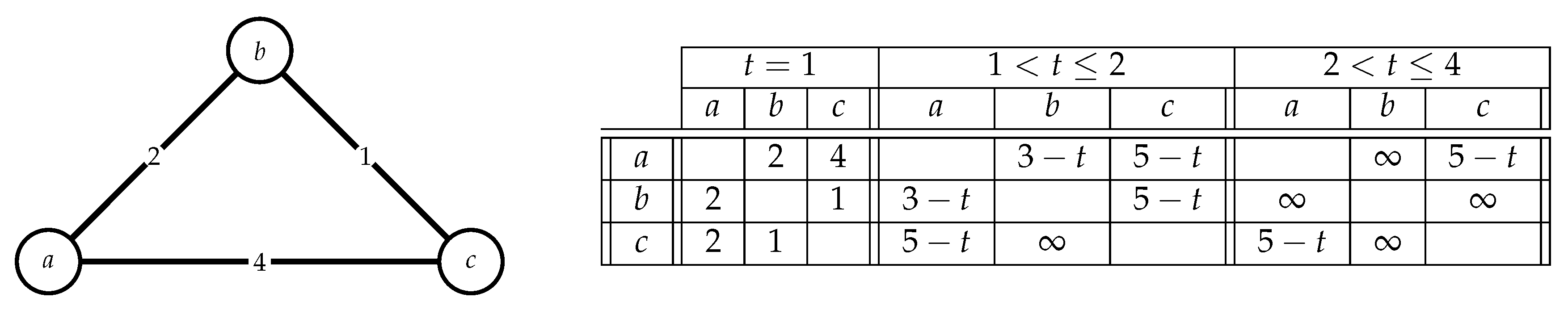
However, if the temporal information is just ignored, we can lose important properties of the graph and we can even deduce wrong consequences. For example, in the case of the temporal undirected graph shown in the left part of Figure 1, if we ignore the temporal information associated with the edges, we can erroneously conclude that there exists a path starting from node a, arriving at node c, and visiting the other node b. However, this path does not correspond to a temporally-feasible path, since the edge connecting node a to node b appears after the edge connecting b to c: in other words, when we arrive in b it is too late to take the edge towards c. It is then important to analyze temporal graph properties by taking into account the temporal information concerning the time intervals in which specific edges appear in the graph. For this reason, the community has rethought several classical definitions of graph theory in terms of temporal graphs [15,16,17].
One of such definition is the one of closeness centrality, which has been repeatedly reconsidered in the case of temporal graphs [18,19,20,21,22,23,24,25,26,27]. In several of these papers, the authors refer to the classical definition of closeness centrality (that is, the one based on the average temporal distance), but in many cases, they actually consider the temporal analogue of the harmonic closeness centrality. In both cases, however, the first step to perform in order to rethink the definition of closeness in terms of temporal graphs consists of defining the temporal distance between two nodes. Even if different notions of distance have been introduced while working with temporal graphs (see, for example, [28]), in this paper, we will focus only on one specific distance definition, which is, in our opinion, one of the most natural ones: that is, the time duration of the earliest arrival path starting no earlier than a specific time instant. This definition is motivated, for example, by the following typical query one could pose to a public transport network: if I want to leave no earlier than time t, how long does it take to me to go from a (bus/metro/train) station to another station?
More precisely, for any time instant t, a temporal t-path (also called t-journey) is a sequence of edges such that the first edge appears no earlier than t and each edge appears later than the edges preceding it. Its arrival time is the appearing time of its last edge and its duration is the difference between its arrival time and t (plus one in order to include the traveling time along the last edge). The t-distance d t ( u , v ) from a node u to a node v is then the minimum duration of any temporal t-path connecting u to v and having the smallest arrival time (once again, if there is no t-path from u to v, we will assume that d t ( u , v ) = ). For instance, in the case of the temporal triangle in the left part of Figure 1, we have that d 1 ( c , a ) = 2 1 + 1 = 2 , while d 2 ( c , a ) = 4 2 + 1 = 3 : indeed, if we insist in leaving after time 1, we cannot arrive at a before time 4. Note that, for any t ( 2 , 4 ] , d t ( b , a ) = d t ( b , c ) = , since there are no temporal edges incident to b with appearing time greater than 2.
Once we have a definition of distance from a node to another node, we can define the notion of temporal closeness centrality of a node u at a given time instant t by simply applying the harmonic definition of closeness in the case of a static graph (see, for example, [9]). Note that we refer to the harmonic closeness centrality, since, as in the case of weakly connected directed graphs, this definition allows us to deal with the fact that two nodes might not be connected by a temporal path. More precisely, the t-closeness of a node u is defined as C t ( u ) = 1 n 1 v V : v u 1 d t ( u , v ) . In [22], the evolution of C t ( u ) was analysed in the case of two social networks (an e-mail graph and a contact graph). To this aim, the authors used an algorithm (inspired by [29]) for computing the t-closeness of a node of a temporal graph, whose time complexity is linear in the number m of temporal edges and whose space complexity is linear in the number n of nodes. For example, we can apply this algorithm to analyse and compare the evolution of the t-closeness in the case of two actors, by referring to the IMDB collaboration graph, where the nodes are the actors and the temporal edges correspond to collaborations in the same (non TV) movie (the appearing time of an edge is the year of the movie). In the left part of Figure 2, we show the evolution of the t-closeness of Christopher Lee and Eleanor Parker (two actors who were alive approximately in the same period) (Note that the t-closeness is greater than zero even when t is less than the birth year of the corresponding actor. This is not a contradiction, since, in general, a temporal edge may contribute to the t-closeness of a node for all t preceding the appearing time of the temporal edge itself). As can be seen, the two plots are quite similar until the end of the sixties (even if the plot of Parker has a smaller peak). Successively, Parker drastically reduced her activity (indeed, after The sound of music in 1965, she participated to only six not very successful movies), while Lee had two other growing periods (most likely, the second one is related to his participation to the Star Wars and the The Lord of the Rings sagas). The figure thus suggests that Lee has been more “important” than Parker.
In order to capture this idea formally, we introduce a global temporal closeness centrality of a node u in a given time interval [ t 1 , t 2 ] which is based on computing the integral of C t ( u ) over that interval. That is, for any node u in the graph, we compute and analyse the temporal closeness C ( u ) of u, which is defined as
C ( u ) = 1 t 2 t 1 t 1 t 2 C t ( u ) d t
(intuitively, C ( u ) can be seen as the Area Under Curve (AUC) value of the function C t ( u ) ). This is similar to what is done in [18] for the betweenness centrality (which is connected to the number of shortest paths that pass through a node): since their betweenness definition depends on the time at which a node is considered, they average it to obtain a global value. Here the integral is the natural equivalent of the average, for a continuous function. For example, the closeness of Christopher Lee is approximately equal to 0.005, while the closeness of Eleanor Parker is approximately equal to 0.003, thus confirming the previous intuition that Lee is more central than Parker. The right part of Figure 2, instead, shows the top 20 nodes in the public transport temporal graph of Paris with respect to the temporal closeness centrality measure (the used graph is derived by the data set published in [30], and successively adapted to the temporal graph framework in [31]).

1.1. Our Results

Our first contribution is the design and analysis of an algorithm for computing the temporal closeness of a node of a temporal graph in a given time interval, whose time complexity is linear in the number m of temporal edges and whose space complexity is linear in the number n of nodes. This algorithm, which is an appropriate modification of the one used in [22] and adapted from [29], can be seen as a temporal version of the classical breadth-first search algorithm. Computing the temporal closeness of all nodes in order to compare them and find the nodes with highest temporal closeness can, hence, be done in time O ( n m ) , by applying n times the algorithm for computing the temporal closeness of a node. This time complexity, however, is much too high in the case of large temporal graphs.
Our second and more important contribution is showing that the algorithm for computing the temporal closeness of a node can be modified in order to obtain a backward version of the algorithm itself, which allows us to compute the “contribution” C ( u , d ) of a specific node d to the temporal closeness of any other node u. By using this algorithm (which is inspired by the earliest arrival profile algorithms of [32]), we can then implement a temporal version of the sampling algorithm introduced in [4] in order to approximate the closeness in static graphs. In particular, for a temporal graph with n nodes and m temporal edges, we can compute an estimate of the temporal closeness of all its nodes whose absolute error is bounded by ϵ in time O log n ϵ 2 m , which significantly improves over the time complexity of applying n times the algorithm for computing the temporal closeness of a node, that is, O ( n m ) .
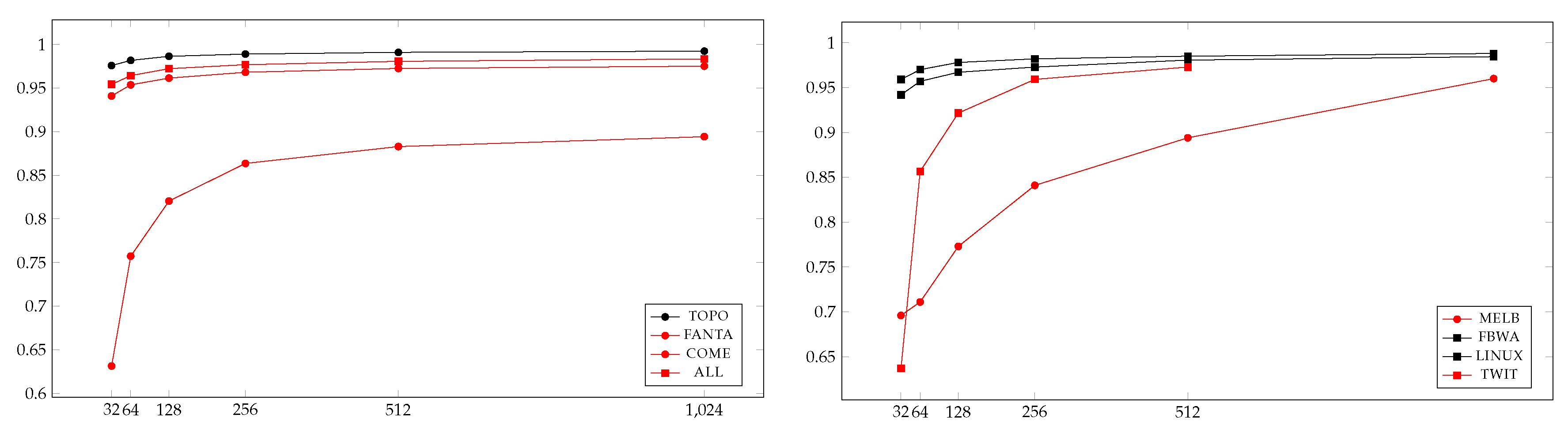
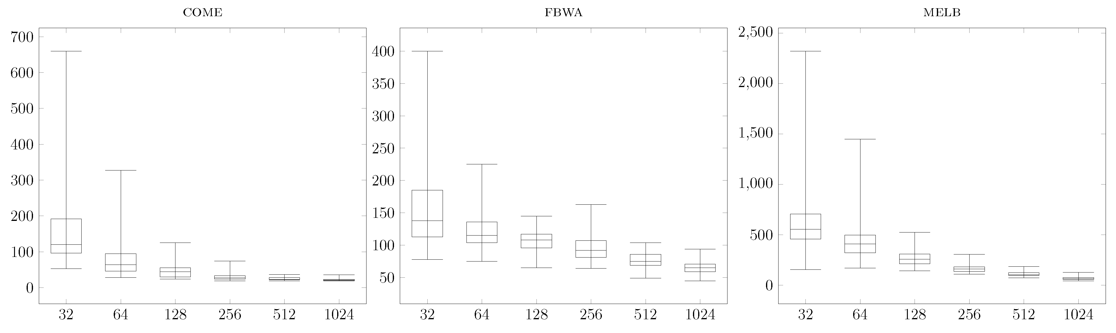
There is a natural way of using this temporal closeness estimation to empirically find the exact top-k nodes according to our temporal closeness metric. This approach simply consists in running our estimate temporal closeness computation algorithm, in finding the top-K nodes for the estimated temporal closeness, with K > k , and in computing the exact temporal closeness of these nodes. Our third contribution is an extensive experimental validation of this approach with a dataset of 45 medium/large temporal graphs. Indeed, we show empirically that using this method we can retrieve the actual top-100 nodes of all large graphs we have considered by choosing K = 1024 , that is (with a little abuse of notation), in time O ( 2048 × m ) , which is between 10 and 100 times faster than computing the temporal closeness of all nodes.

1.2. Other Related Work

Besides the references given above, our paper is related to all work on the definition and computation of different temporal centrality measures, such as the temporal betweenness centrality defined in [33], the f-PageRank centrality defined in [34], or the temporal reachability used in [35], just to mention some recent ones. The authors of [36], instead, study the evolution of the closeness centrality for static graphs and propose efficient algorithms for computing it. In the case of static graphs, an approach based on the sampling approximation algorithm of [4], in order to select the candidates for which computing the exact closeness, was proposed in [37]: its complexity is, however, still quite high, that is, O ˜ ( n 2 / 3 m ) (under the rather strong assumption that closeness values are uniformly distributed between 0 and the diameter). Still, in the case of static graphs, in [38] the authors identify the candidates by looking for central nodes with respect to a “simpler” centrality measure (for instance, degree of nodes).

1.3. Structure of the Paper

In the rest of this section, we give all the necessary definitions concerning temporal paths, temporal distances and temporal closeness (these definitions are mostly inspired by [16,28,39]). In Section 2 we introduce and analyze our algorithm for computing the temporal closeness of a node of a temporal graph in a given time interval, while in Section 3 we describe and analyze the backward version of this algorithm and we show how this version can be used in order to obtain an error-guaranteed estimate of the temporal closeness of all the nodes of a temporal graph. In these two sections, we assume that the temporal edges have all distinct appearing times: in Section 4, we show how our algorithms can be adapted (without worsening the time and space complexity) to the more general and more realistic case in which multiple edges can appear at the same time. In Section 5 we experimentally validate our approximation algorithm and we show how it can be applied to the problem of finding the top nodes in real-world medium/large temporal graphs. Finally, in Section 6 we conclude by suggesting some research directions and possibly other applications of our backward temporal breadth-first search algorithm.

1.4. Definitions and Notations

A temporal graph is a pair G = ( V , E ) , where V is the set of nodes and E is the set of temporal edges. A temporal edge e E is a triple ( u , v , t ) , where u , v V are the source and destination nodes of the edge, respectively, and t N is the appearing time of the edge. If the temporal edges are bidirectional, then ( u , v , t ) can be also written as ( v , u , t ) . Let t α (respectively, t ω ) denote the minimum (respectively, maximum) appearing time of a temporal edge in E. The time horizon T ( G ) of a temporal graph G is the interval [ t α , t ω ] of real numbers no smaller than t α and no greater than t ω . In this paper, we will assume that the temporal edges are given to the algorithms one after the other (similarly, to the streaming model) either in non-decreasing or in non-increasing order with respect to the appearing time.
A temporal path P (also called a temporal walk [17]) in a temporal graph G = ( V , E ) from a node u V to a node v V is a sequence of temporal edges e 1 = ( u 1 , v 1 , t 1 ) , e 2 = ( u 2 , v 2 , t 2 ) , , e k = ( u k , v k , t k ) such that u = u 1 , v = v k , and, for each i with 1 < i k , u i = v i 1 and t i t i 1 + 1 . The length of a temporal path is the number of temporal edges included in it. The starting time (respectively, ending time) of a temporal path P , denoted by σ ( P ) (respectively, η ( P ) ), is equal to the appearing time of the first (respectively, last) temporal edge in the path. Given a time t T ( G ) and two nodes u and v, we will denote by P ( u , v , t ) the set of all temporal paths P from u to v such that σ ( P ) t . Among all these temporal paths, in this paper we will distinguish the ones which allow us to arrive as early as possible.
Definition 1.
Given a temporal graph G = ( V , E ) , two nodes u and v in V, and a time t T ( G ) , a path P P ( u , v , t ) is said to be an earliest arrival t-path if η ( P ) = min { η ( P ) : P P ( u , v , t ) } .
Given a time t T ( G ) and two nodes u and v, the t-duration of a path P P ( u , v , t ) is defined as δ ( P ) = η ( P ) t + 1 . Hence, an earliest arrival t-path is also a path in P ( u , v , t ) with minimum t-duration. For this reason, we will also call these paths the shortest t-paths from u to v.
Definition 2.
Given a temporal graph G = ( V , E ) , two nodes u and v in V, and a time t T ( G ) , the t-distance d t ( u , v ) from u to v is equal to the t-duration of any shortest t-path from u to v (by convention, if P ( u , v , t ) = , then we set d t ( u , v ) = ).
Once we have introduced the notion of t-distance, we can also define the analog of the harmonic closeness centrality in static graphs as follows.
Definition 3.
Given a temporal graph G = ( V , E ) , a node u, and a time t T ( G ) , the t-closeness of u is defined as
C t ( u ) = 1 n 1 v V : u v 1 d t ( u , v ) .
The (temporal) closeness of u in T ( G ) is then defined as
C ( u ) = 1 t ω t α t α t ω C t ( u ) d t .

An Example

Let us consider the temporal graph shown in the left part of Figure 1. In this case, t α = 1 , t ω = 4 , and T ( G ) = [ 1 , 4 ] . As shown in the right part of the figure, for any t [ 1 , 2 ] , the duration of a shortest t-path from node a to node b is equal to d t ( a , b ) = 2 t + 1 = 3 t , while, for any t ( 2 , 4 ] , this duration is infinity since there is no t-path from node a to node b. On the other hand, for any t [ 1 , 4 ] , the duration of a shortest t-path from node a to node c is equal to d t ( a , c ) = 4 t + 1 = 5 t . Hence, the closeness of node a is equal to
C ( a ) = 1 2 1 3 1 2 1 3 t + 1 5 t d t + 2 4 1 5 t d t = 1 6 ln 2 1 + ln 4 3 + ln 3 1 0.35 .
Analogously, we can verify that the closeness of node b is C ( b ) 0.16 , and that the closeness of node c is C ( c ) 0.23 .

2. Computing the Closeness

In this section, we propose an algorithm for computing exactly the closeness of a node u of a temporal graph G. This algorithm can be seen as a temporal version of the breadth-first search algorithm starting from a source node s, in which the temporal edges are scanned in non-decreasing order with respect to their appearing time. In the following, we assume that the appearing times of all temporal edges are distinct: the algorithm can be adapted to the case in which this assumption is not satisfied, as we will see below. Moreover, we assume that the temporal graph is directed: if this is not the case, we simply have to examine each edge twice by inverting the source and the destination.
The algorithm maintains, for each node x of G, a triple τ x = ( l x , r x , a x ) , which indicates that, for any time instant t in ( l x , r x ] , any earliest arrival t-path P from s to x has ending time η ( P ) equal to a x (see Algorithm 1). At the beginning, we do not know anything about the reachability of a node x from s: hence, we set the arrival time of x equal to for an arbitrary time interval (for example, ( t α 2 , t α 1 ] ) preceding t α (line 1). When we read a new temporal edge ( x , y , t ) , we first set τ s = { ( t 1 , t , t 1 ) } , since, clearly, the source node is always reachable even before the appearance of the edge (line 2). Let τ x = ( l x , r x , t x ) and τ y = ( l y , r y , t y ) be the two triples associated with x and y, respectively. If r x > r y , then we add to the closeness of s the contribution of node y corresponding to the interval ( l y , r y ] (line 3) and we update the triple associated with y by setting τ y = ( r y , r x , t ) (line 4). This update is justified by Lemma 1. When all temporal edges have been read, we add to the closeness of s the contribution of a node x corresponding to the interval ( l x , r x ] (line 5), which is the last interval for which the earliest arrival time has been computed. The way of computing the contribution to the closeness of s (lines 3 and 5) is justified by the proof of Theorem 1.
Lemma 1.
Let G = ( V , E ) be a temporal graph and s V . For any u V with u s , let Ξ u = τ u , 0 , τ u , 1 , , τ u , h u be the sequence of triples τ u , i = ( l u , i , r u , i , a u , i ) such that l u , 0 = t α 2 , r u , 0 = t α 1 , a u , 0 = , and, for 1 i h u , ( l u , i , r u , i , a u , i ) is the triple assigned to τ [ u ] at the i-th execution of line 4 with y = u during the running of Algorithm 1 with input G and s (note that h u = 0 if this line is never executed with y = u ). Then, for any u V with u s , the intervals ( l u , i , r u , i ] , for 0 i h u , form a partition of the interval ( t α 2 , r u , h u ] , and, for any t T ( G ) ,
d t ( s , u ) = a u , i t + 1 i f   t ( l u , i , r u , i ] w i t h   1 i h u , o t h e r w i s e .
Algorithm 1: Algorithm for computing the closeness of a node
Algorithms 13 00211 i001
Proof. 
We prove the lemma by induction on the number k of temporal edges that have been read. In particular, for any k with 0 k | E | , let A ( k ) be the following statement.
For any u V with u s , let Ξ u k = τ u , 0 , τ u , 1 , , τ u , h u k be the prefix of Ξ u containing the triples assigned to τ [ u ] at line 4 with y = u after having read k edges. The intervals ( l u , i , r u , i ] , for 0 i h u k , form a partition of the interval ( t α 2 , r u , h u k ] , and, for any t [ t α , r u , h u k ] , if t ( l u , i , r u , i ] then d t ( s , u ) = a u , i t + 1 .
We now prove by induction on k that A ( k ) is true for any k with 0 k | E | .
Base case. k = 0 . In this case, no edge has been read yet and, hence, line 4 has never been executed with y = u . We then have that, for any u V with u s , h u 0 = 0 , Ξ u 0 = τ u , 0 with τ u , 0 = ( t α 2 , t α 1 , ) , and, hence, ( l u , 0 , r u , 0 ] = ( t α 2 , t α 1 ] = ( t α 2 , r u , h u 0 ] . Moreover, the interval [ t α , r u , h u 0 ] = [ t α , t α 1 ] is empty and the condition on the t-distances is “vacuosly” true. Hence, A ( 0 ) is true.
Induction step. Given k with 1 k | E | , suppose that A ( k 1 ) is true. We now prove that A ( k ) is also true. Let e = ( x , y , t ) be the k-th temporal edge read by the algorithm. Clearly, this edge has no influence on any other node than y (since the graph is directed). Hence, we have just to prove that the value of τ [ y ] is correctly updated. By the induction hypothesis, we know that the current value of τ [ y ] = ( l y , r y , a y ) is such that, for any t [ t α , r y ] , the ending time of any earliest arrival t -path from s to y is at most a y < t . Hence, the edge e cannot improve these ending times since its appearing time is t. Analogously, we know that the current value of τ [ x ] = ( l x , r x , a x ) is such that a x < t is the ending time of any earliest arrival t -path from s to x with t ( l x , r x ] . If r x r y , the edge e does not add any information for the node y, since we already know the ending time of any earliest arrival t -path from s to y, for any t r y 
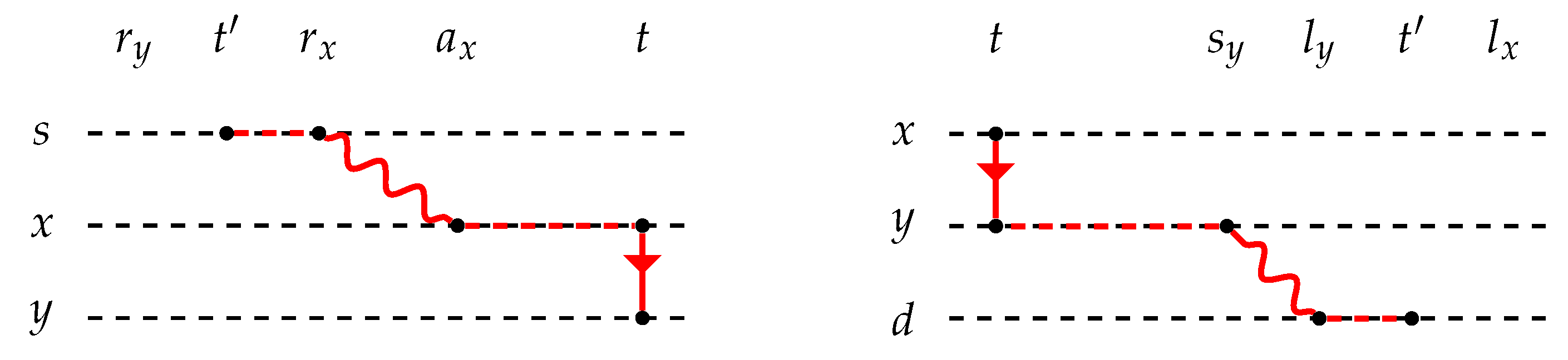
. On the contrary (see the left part of Figure 3), if r x > r y , then, for any time instant t ( r y , r x ] (for which we did not know yet the corresponding ending time of any earliest arrival t -path from s to y), we can now say that we can first reach x (at time a x with r x a x < t ), and then wait until the temporal edge e appears to move to y at time t: hence, for all these time instants, the earliest arrival time at y can now be set equal to t, that is, the value of τ [ y ] becomes ( r y , r x , t ) (note that subsequent edges cannot improve this value since their appearing times are greater than t). Hence, if Ξ y k 1 = τ y , 0 , τ y , 1 , , τ u , h y k 1 , we have that Ξ y k = τ y , 0 , τ y , 1 , , τ u , h y k with h y k = h y k 1 + 1 and τ u , h y k = ( r y , r x , t ) . By induction hypothesis, the intervals ( l y , i , r y , i ] , for 0 i h y k 1 , form a partition of the interval ( t α 2 , r y , h y k 1 ] : by adding the triple ( r y , r x , t ) , we obtain a partition of the interval ( t α 2 , r y , h y k ] (since r y = r y , h y k 1 and r x = r y , h y k ). From the previous argument, it also follows that, for any t [ t α , r y , h y k ] , if t ( l y , i , r y , i ] then d t ( s , y ) = a y , i t + 1 . We have thus proved that A ( k ) is satisfied.
The lemma follows from the fact that its statement is exactly equivalent to A ( | E | ) . □
Theorem 1.
Let G = ( V , E ) be a temporal graph and s V . Algorithm 1 with input G and s correctly computes the closeness of s in G. If the temporal edges are already ordered in increasing order with respect to their appearing time, then the complexity of the algorithm is O ( | E | ) time and O ( | V | ) space.
Proof. 
From Lemma 1, it follows that, with respect to the node u, the interval I = ( t α 2 , r u , h u ] is partitioned into h u + 1 intervals ( l u , i , r u , i ] , such that, for any t [ t α , t ω ] , if t ( l u , i , r u , i ] , then d t ( s , u ) = a u , i t + 1 . That is, each time instant t ( l u , i , r u , i ] [ t α , t ω ] contributes to the closeness of s with the value 1 a u , i t + 1 . Hence, the closeness of s is equal to
C ( s ) = 1 ( n 1 ) ( t ω t α ) u V : u s i = 0 h u max ( t α , l u , i ) max ( t α , r u , i ) 1 a u , i t + 1 d t = 1 ( n 1 ) ( t ω t α ) u V : u s i = 1 h u ln a u , i max ( t α , l u , i ) + 1 a u , i max ( t α , r u , i ) + 1 .
Note that we used the maximum function in order to deal with the first interval whose left extreme is smaller than t α and whose right extreme can also be smaller than t α (whenever u is not reachable from s in the interval [ t α , t ω ] ). Observe that the interval ( r u , h u , t ω ] might be non empty: however, if this the case, then we can conclude that if we start from s at time t in this interval, then we cannot reach u. That is, d t ( s , u ) = for any t ( r u , h u , t ω ] and, hence, this interval does not contribute to the closeness of s. Hence, Algorithm 1 correctly computes the closeness of node s.
The time complexity of the algorithm is clearly O ( | E | ) , since each temporal edge is analyzed one time only, and the update operation requires constant time. The space complexity is linear in the number of nodes, since (apart from the value C), for each node u, we have to maintain just three numbers corresponding to the current value of τ [ u ] . □
From the previous theorem, it follows that if we want to compute the closeness of all nodes, this would take time O ( | V | | E | ) , since we have to execute Algorithm 1 for each source node s. This time complexity may turn out to be not acceptable in the case of real-world large size temporal graphs. That is why in the next section, we propose an analog of the sampling algorithm used for approximating the closeness in the case of static graphs [4], based on an appropriate modification of Algorithm 1.

3. Approximating the Closeness

In order to approximate the closeness in temporal graphs, we first need to introduce the notion of the latest starting path. To this aim, given a time t T ( G ) and two nodes u and v, we will denote by P ( u , v , t ) the set of all temporal paths P from u to v such that η ( P ) t .
Definition 4.
Given a temporal graph G = ( V , E ) , two nodes u and v in V, and a time t T ( G ) , a path P P ( u , v , t ) is said to be the latest starting t-path if σ ( P ) = max { σ ( P ) : P P ( u , v , t ) } .
Moreover, we need to define the contribution of a destination node d to the closeness of another node u.
Definition 5.
Given a temporal graph G = ( V , E ) and two distinct nodes d and u, the contribution of d to the closeness of u is defined as
C ( u , d ) = 1 t ω t α t α t ω 1 d t ( u , d ) d t .
By convention, we also set C ( u , u ) = 0 , for any node u V .
We now introduce a sort of backward version of Algorithm 1 (which can be seen as an adaptation of the earliest arrival profile algorithms proposed in [32]), which has to be applied to a destination node d, and that will allows us to compute, for any other node x, the contribution of d to the closeness of x (that is, C ( x , d ) ) and, hence, to adapt to temporal graphs the well-known sampling technique already used in the case of classical graphs. Differently from the case of Algorithm 1, we assume that the temporal edges are scanned in non-increasing order with respect to their appearing times. Once again, we assume that the appearing times of all temporal edges are distinct (we will see in the next section how the algorithm can be adapted to the case in which this assumption is not satisfied), and that the temporal graph is directed (if this not the case, we simply have to examine each edge twice by inverting the source and the destination). The algorithm maintains, for each node x of G, a triple τ x = ( l x , r x , s x ) , which indicates that, for any time instant t in [ l x , r x ) , any latest starting t-path P from x to d has starting time σ ( P ) equal to s x (see Algorithm 2). At the beginning, we do not know anything about the reachability of d from a node x: hence, we set the starting time of x equal to for an arbitrary time interval (for example, [ t ω + 1 , t ω + 2 ) ) following t ω (line 1). When we read a new temporal edge ( x , y , t ) , we first set τ d = { ( t , t + 1 , t + 1 ) } , since, clearly, the destination node can always reach itself even starting after the appearance of the edge (line 2). Let τ x = ( l x , r x , s x ) and τ y = ( l y , r y , s y ) be the two triples associated with x and y, respectively. If l x > l y , then we add to C ( x , d ) the contribution corresponding to the interval [ l x , r x ) (line 3) and we update the triple associated with x by setting τ x = ( l y , l x , t ) (line 4). This update is justified by Lemma 2. When all temporal edges have been read, for each node x, we add to C ( x , d ) the contribution corresponding to the interval [ l x , r x ) and to the interval [ t α , l x ) (line 5), which are the last intervals for which the latest starting time has been computed. The way of computing the contribution to C ( x , d ) (lines 3 and 5) is justified by the proof of Theorem 2.
Algorithm 2: Algorithm for computing the closeness contribution of a node to all the others
Algorithms 13 00211 i002
Lemma 2.
Let G = ( V , E ) be a temporal graph and d V . For any u V with u d , let Ξ u = τ u , 1 , τ u , 2 , , τ u , h u , τ u , h u + 1 be the sequence of triples τ u , i = ( l u , i , r u , i , s u , i ) such that l u , h u + 1 = t ω + 1 , r u , h u + 1 = t ω + 2 , s u , h u + 1 = , and, for 1 i h u , ( l u , i , r u , i , s u , i ) is the triple assigned to τ [ u ] at the ( h u + 1 i ) -th execution of line 4 with x = u during the running of Algorithm 2 with input G and d (note that h u = 0 if this line is never executed with x = u ). Then, for any u V with u d , the intervals [ l u , i , r u , i ) , for i i h u + 1 , form a partition of the interval [ l u , 1 , t ω + 2 ) , and, for any t T ( G ) ,
d t ( u , d ) = r u , i t + 1 i f   s u , i < t s u , i + 1   w i t h   1 i h u , o t h e r w i s e .
Proof. 
We prove the lemma by induction on the number k of temporal edges that have been read. In particular, for any k with 0 k | E | , let S ( k ) be the following statement.
For any u V with u s , let Ξ u k = τ u , h u k , , τ u , h u + 1 be the suffix of Ξ u containing the triples assigned to τ [ u ] at line 4 with x = u after having read k edges. The intervals [ l u , i , r u , i ) , for h u k i h u + 1 , form a partition of the interval [ l u , h u k , t ω + 2 ) , and, for any t [ l u , h u k , t ω ] , if s u , i < t s u , i + 1 then d t ( u , d ) = r u , i t + 1 .
We now prove by induction on k that S ( k ) is true for any k with 0 k | E | .
Base case. k = 0 . In this case, no edge has been read yet and, hence, line 4 has never been executed with x = u . We then have that, for any u V with u d , h u 0 = h u + 1 , Ξ u 0 = τ u , h u + 1 with τ u , h u + 1 = ( t ω + 1 , t ω + 2 , ) , and, hence, [ l u , h u + 1 , r u , h u + 1 ) = [ t ω + 1 , t ω + 2 ) = [ l u , h u 0 , t ω + 2 ) . Moreover, the interval [ l u , h u 0 , t ω ] = [ t ω + 1 , t ω ] is empty and the condition on the t-distances is “vacuosly” true. Hence, S ( 0 ) is true.
Induction step. Given k with 1 k | E | , suppose that S ( k 1 ) is true. We now prove that S ( k ) is also true. Let e = ( x , y , t ) be the k-th temporal edge read by the algorithm. Clearly, this edge has no influence on any other node than x (since the graph is directed). Hence, we have just to prove that the value of τ [ x ] is correctly updated. By the induction hypothesis, we know that the current value of τ [ x ] = ( l x , r x , s x ) is such that, for any t [ l x , t ω ] , the starting time of any latest starting t -path from x to d is at least s x > t . Hence, the edge e cannot improve these starting times since its appearing time is t. Analogously, we know that the current value of τ [ y ] = ( l y , r y , s y ) is such that s y > t is the starting time of any latest starting t -path from y to d with t [ l y , r y ) . If l y l x , the edge e does not add any information for the node x, since we already know the starting time of any latest starting t -path from x to d, for any t l x . On the contrary (see the right part of Figure 3), if l y < l x , then, for any time instant t [ l y , l x ) (for which we did not know yet the corresponding latest starting time from x), we can now say that we can first reach y (at time t with t < s y l y by using the temporal edge e), and then wait until starting the path from y to d at time s y : hence, for all these time instants, the latest starting time at x can now be set equal to t, that is, the value of τ [ x ] becomes ( l y , l x , t ) (note that subsequent edges cannot improve this value since their appearing times are smaller than t). Hence, if Ξ y k 1 = τ x , h x k 1 , , τ u , h x + 1 , we have that Ξ x k = τ x , h x k , τ x , h x k 1 , , τ u , h x + 1 with h x k = h x k 1 1 and τ u , h x k = ( l y , l x , t ) . By the induction hypothesis, the intervals [ l x , i , r x , i ) , for h x k 1 i h x , form a partition of the interval [ l x , h x k 1 , t ω + 2 ) : by adding the triple ( l y , l x , t ) , we obtain a partition of the interval [ l x , h x k , t ω + 2 ) (since l x = l x , h x k 1 and l y = r x , h x k ). From the previous argument, it also follows that, for any t [ l x , h x k , t ω ] , if s x , i < t s x , i + 1 then d t ( x , d ) = r x , i t + 1 . We have thus proved that S ( k ) is satisfied.
The lemma follows from the fact that its statement is exactly equivalent to S ( | E | ) . □
Theorem 2.
Let G = ( V , E ) be a temporal graph and d V . Algorithm 2 with input G and d correctly computes, for any u V with u d , the value C ( u , d ) . If the temporal edges are already ordered in decreasing order with respect to their appearing time, then the complexity of the algorithm is O ( | E | ) time and O ( | V | ) space.
Proof. 
From Lemma 2, it follows that, with respect to the node u, the interval I = [ l u , 1 , t ω + 2 ] is partitioned into h u + 1 intervals [ l u , i , r u , i ) , such that, for any t [ t α , t ω ] , if s u , i < t s u , i + 1 , then d t ( u , d ) = r u , i t + 1 . That is, each time instant t ( s u , i , s u , i + 1 ] [ t α , t ω ] contributes to C ( u , d ) with the value 1 r u , i t + 1 . Hence, we have that
C ( u , d ) = 1 t ω t α t α min ( s u , 1 , t ω ) 1 l u , 1 t + 1 d t + i = 1 h u s u , i min ( s u , i + 1 , t ω ) 1 min ( r u , i , t ω ) t + 1 d t = 1 t ω t α ln l u , 1 t α + 1 l u , 1 min ( s u , 1 , t ω ) + 1 + i = 1 h u ln min ( r u , i , t ω ) s u , i + 1 min ( r u , i , t ω ) min ( s u , i + 1 , t ω ) + 1 .
Note that we used the minimum function in order to deal with the last interval whose right extreme is greater than t ω and whose left extreme can also be greater than t ω (whenever u cannot reach d in the interval [ t α , t ω ] ). Note also that the interval [ t α , l u , 1 ) might be non empty: if this the case, then we can conclude that if we start from u at time t in this interval, then we cannot reach d before l u , 1 . That is, d t ( u , d ) = l u , 1 t + 1 for any t [ t α , l u , 1 ) and, hence, this interval contributes to C ( u , d ) with the first integral in the previous equation. Hence, Algorithm 2 correctly computes the contribution C ( u , d ) of node d to the closeness of node u.
The time complexity of the algorithm is clearly O ( | E | ) , since each temporal edge is analyzed once only, and the update operation requires constant time. The space complexity is linear in the number of nodes, since, for each node u, we have to maintain (apart from the value C) just four numbers corresponding to the current value of τ [ u ] and to the starting value of the previous tuple. □
From the definition of closeness and of C ( u , d ) , it follows that
C ( u ) = 1 n 1 d V C ( u , d ) .
This formula immediately suggests the following definition of an estimator of the closeness of a node.
Definition 6.
Given a temporal graph G = ( V , E ) , a node u, and a (multi)set X = { x 1 , , x h } of vertices in V, we define the closeness X-estimator of u in T ( G ) as
C X ( u ) = 1 n 1 n h i = 1 h C ( u , x i ) .
Theorem 3.
Let G = ( V , E ) be a temporal graph and X V be a randomly chosen (multi)set of h nodes in G. If h = Θ ( log n / ϵ 2 ) , then, for any node u V , | C ( u ) C X ( u ) | ϵ with high probability.
The proof of the above theorem uses the same techniques of [4], and is very similar to the one given in [40] to analyze the absolute error of a sampling-based algorithm for computing distance distribution approximations in static graphs. For the sake of completeness, we give the complete proof. As a first step, the following lemma shows that the closeness estimator is unbiased.
Lemma 3.
Given a temporal graph G = ( V , E ) and a uniformly randomly chosen node x V , the expected value of C { x } ( u ) is equal to C ( u ) .
Proof. 
Since x has been randomly chosen in a uniform way, we have that
E [ C { x } ( u ) ] = 1 n d V C { d } ( u ) .
From the definition of the estimator and from the fact that h = 1 , it follows that
E [ C { x } ( u ) ] = 1 n 1 n 1 n d V C ( u , d ) = 1 n 1 d V C ( u , d ) = C ( u ) .
The lemma is thus proved. □
In order to prove Theorem 3, we make use of the following application of the Hoeffding’s inequality (see, for example, [41]).
Theorem 4.
If A 1 , A 2 , , A h are independent random variables such that μ = E [ i = 1 h A i / h ] and, for each i, 0 A i 2 , then, for any ϵ 0 ,
P r i = 1 h A i h μ ϵ 2 e h ϵ 2 2 .
Proof Theorem 3. 
Given a temporal graph G = ( V , E ) , a node u, and a randomly chosen (multi)set X of nodes in V with X = { x 1 , , x h } , we apply the above theorem by setting A i = C { x i } ( u ) , for each i with 1 i h . From Lemma 3, it follows that
μ = E i = 1 h A i / h = E i = 1 h C { x i } ( u ) / h = 1 h i = 1 h E C { x i } ( u ) = 1 h i = 1 h C ( u ) = C ( u ) .
Moreover, from the definition of the estimator and from the fact that we can assume that the number n of nodes is at least equal to 2, we have that, for each i with 1 i h ,
0 A i = C { x i } ( u ) 2 .
Finally, we also have that
i = 1 h A i h = 1 h i = 1 h C { x i } ( u ) = 1 h n n 1 i = 1 h C ( u , x i ) = 1 n 1 n h i = 1 h C ( u , x i ) = C X ( u ) .
Hence, from Theorem 4, it follows that, for any ϵ 0 ,
P r C X ( u ) C ( u ) ϵ 2 e h ϵ 2 2 .
By choosing h = 2 log n ϵ 2 , we then have that
P r C X ( u ) C ( u ) ϵ 2 n ,
and the theorem thus follows. □

Finding Top-K Nodes

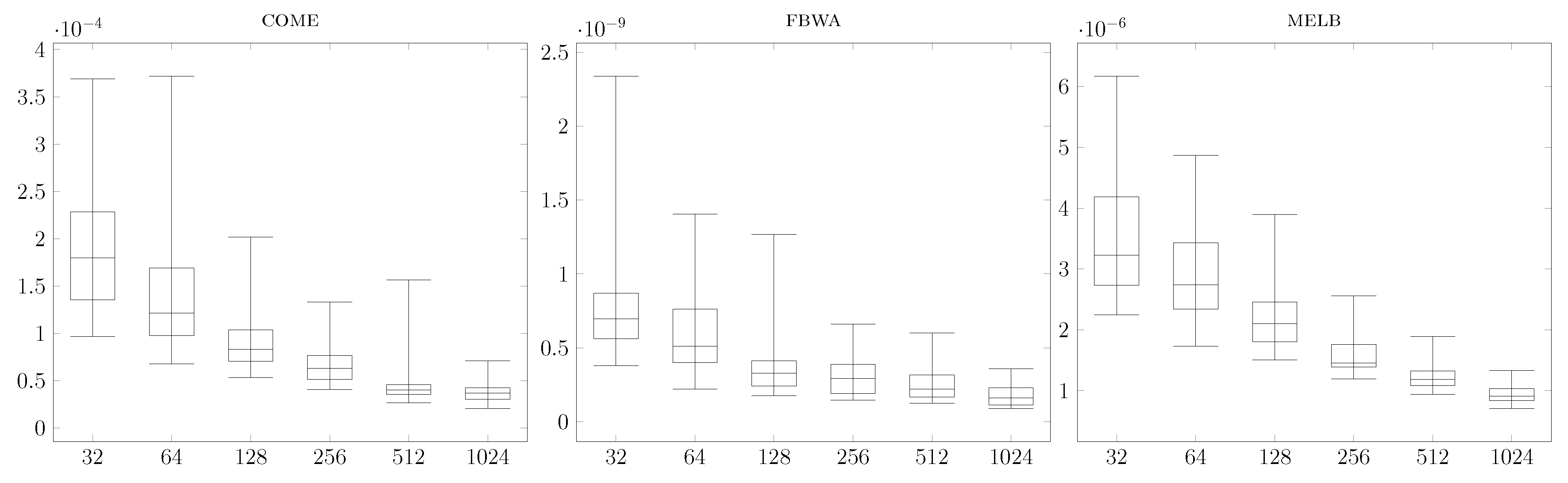
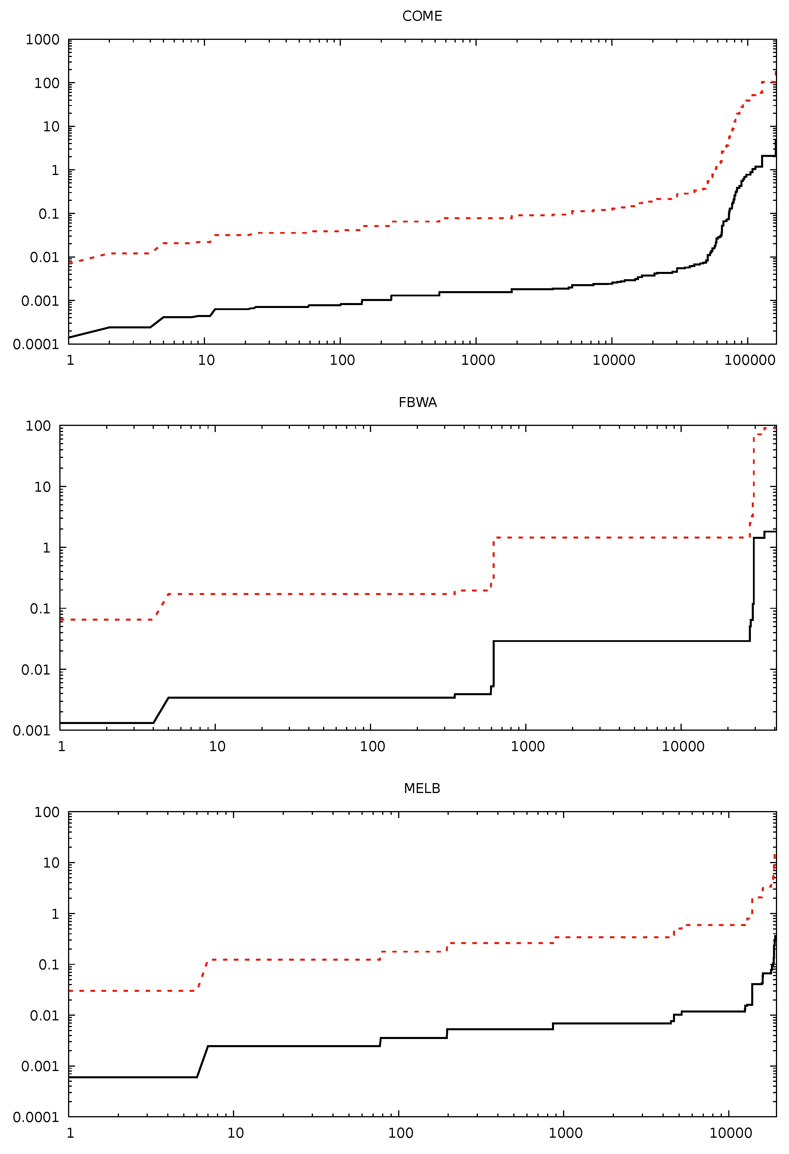
Theorem 3 states that we can approximate the closeness centrality of all nodes of a temporal graph by using a sample of size h, which is logarithmic with respect to the number of nodes. In Section 5, we will show how this approximation method works particularly well for nodes with a high closeness. Based on this observation, a natural strategy for finding the top-k nodes consists of: (a) compute the approximated temporal closeness for all nodes, using a sample size h; (b) rank the nodes according to this estimation and select the top-K nodes, with K > k ; and (c) compute the exact closeness of these K nodes, then rank them and select the top-k nodes. As we will see in Section 5, in practice choosing h = K = 1024 has worked in all cases we have investigated for finding the top-100 nodes. This leads to a total cost proportional to 2048 · m , which is a quite small (between 1 / 10 and 1 / 100 ) fraction of the cost that would be needed to compute the exact closeness for all nodes.

4. How to Deal with Multiple Edges

In the previous sections, we have assumed that, for each time t T ( G ) , there exists at most one edge whose appearing time is equal to t. Clearly, this assumption is not realistic since, in the vast majority of real-world temporal graphs, many edges can appear at the same time. In this section, we show how we can modify Algorithm 2, in order to deal with this more general case (the modification of Algorithm 1 is similar). For the sake of clarity of exposition, we will assume that, for each node u, the algorithm maintains a list I u of triples (instead of just one triple): it is not difficult to show that only the last two triples are really necessary at each iteration of the algorithm, thus assuring that the algorithm itself has linear space complexity.
Let us suppose that a new temporal edge e = ( x , y , t ) arrives, and that the last triple inserted in I x (respectively, I y ) is ( l x , r x , s x ) (respectively, ( l y , r y , s y ) ). This implies that that if we want to arrive at the destination d in the interval [ l x , r x ) (respectively, [ l y , r y ) ), then we cannot start from x (respectively, y) later than s x (respectively, s y ). Remember that, in Algorithm 2, the temporal edges are scanned in non-increasing order with respect to their appearing times: hence, we know that t s x l x < r x (respectively, t s y l y < r y ). We now distinguish the following cases.
  • t < s x t < s y . In this case, neither x nor y has yet used an edge at time t. Hence, we can update the set of intervals as we did in the case of edges with distinct appearing times. That is, if l y < l x , then add to I x the triple ( l y , l x , t ) .
  • t < s x t = s y . In this case, y has already “encountered” an edge at time t. Let ( l y , r y , s y ) be the triple just before ( l y , r y , s y ) in I y (note that l y = r y and that t = s y < s y ). If l y < l x , then we add to I x the triple ( l y , l x , t ) : indeed, since t < s y , we now know that, to arrive at d in the interval [ l y , l x ) , we can start from u at time t (by using the edge e), wait until time s y , and then follow the journey from y to d.
  • t = s x t < s y . In this case, x has already “encountered” an edge at time t. If l y < l x , then we extend to the left the triple of x until l y : indeed, since s x < s y , we now know that, even to arrive at d in the interval [ l y , l x ) , we can start at time t (by using the edge e), wait until time s y , and then follow the journey from y to d.
  • t = s x t = s y . In this case, both x and y have already “encountered” an edge at time t. Let ( l y , r y , s y ) be the triple just before ( l y , r y , s y ) in I y (note that l y = r y and t = s y < s y ). Similarly to the previous case, if l y < l x , then we extend to the left the triple of x until l y .
Note that the modification of the contribution to C ( x , d ) has to be done only in the first two cases (and at the end of the while loop, in order to deal with the leftmost intervals). Note also that the four above cases require constant time, in order to be implemented: hence, the time complexity of the modified algorithm is still linear in the number of temporal edges.

5. Experimental Results

In our experiments, we used 45 medium/large real-world temporal graphs taken from different application domains, that is, collaboration, communication, and transportation domains. For sake of brevity, we describe our results by referring to a sample of our dataset (see Table 1): the entire dataset and the entire set of experimental results are shown in the Appendix A (Table A1). Here, we are going to use the following temporal graphs.
  • topo. The nodes are autonomous systems and the temporal edges are connections between autonomous systems. The appearing time of an edge is the time-point of the corresponding connection [42,43,44].
  • all, come, fant. Every node corresponds to an actor and two actors are connected by their collaboration in a movie, where the appearing time of an edge is the year of the movie. We use the whole temporal collaboration graph and the ones induced by the comedy and the fantasy genres [45].
  • melb. Nodes are transport stops and temporal edges are connections traversed by a public vehicle: the edge appearing time is the arrival time (see [30,31]).
  • fbwa. The nodes of the graph are Facebook users, and each directed temporal edge links the user writing a post to the user whose wall the post is written on [43,44,46].
  • linu. The communication graph of the Linux kernel mailing list. An edge ( u , v , t ) means that user u sent an email to user v at time t [44].
  • twit. Tweets about the migrant crisis of 2015. A directed edge ( u , v , t ) means that user u retweeted a tweet of user v at time t [47,48].
For all graphs (apart from twit), we have computed the exact values of the closeness centrality for all nodes, in order to evaluate the quality of our approximation algorithm and of our ranking algorithm. In the case of twit, we have executed only the approximation algorithm in order to deduce some properties of the graph. Our computing platform is a machine with Intel(R) Xeon(R) CPU E5-2620 v3 at 2.40 GHz, 24 virtual cores, 128 Gb RAM, running Ubuntu Linux version 4.4.0-22-generic. The code was written in Java, using Java 1.8, and it is available at https://github.com/piluc/TemporalCloseness. Hereafter, we will refer to the exact algorithm as exact, and to our approximation algorithm as apx-h, where h denotes the sample size in the definition of the closeness estimator. For each graph in our dataset, we ran apx-h setting h equal to 32, 64, 128, 256, 512, 1024, and repeating each experiment 50 times.

5.1. Running Times

In Table 1 we also report, for each temporal graph, the running times in seconds of exact and apx-1024. In the case of twit, the exact value is an estimation, since the (sequential) execution of the algorithm would have taken approximately three years. In the case of apx-1024 we report the average running time over 50 experiments. We remark that there is very little variability in the execution time of Algorithm 2: hence, a quite precise estimation of the running times of apx-h, for any other value of h, can be obtained by considering the running time t of apx-1024 reported in Table 1, and by computing the value h · t / 1024 (in particular, by taking h equal to the number of nodes, this is the formula used to compute the estimate of the running time of exact with input twit). As can be seen, the improvement of the running time of apx-1024 with respect to exact ranges from one to several orders of magnitude. As expected, this improvement is particularly evident in the case of large graphs, where we are able to compute an approximation of the closeness in less than 16 min instead of more than 5 days for all and in less than 8 h, instead of 3 years for twit.

5.2. Accuracy

In this section, we analyze the accuracy of the estimation performed by apx-h for different h. To this aim, we consider the following measures.
  • Mean Absolute Error (MAE) in each experiment. Namely, for each experiment, we compute v | C X ( u ) C ( u ) | / n , where X is the sample of size h randomly chosen by apx-h. This is guaranteed to be bounded with high probability (see Theorem 3).
  • Relative Error (RE), which is defined, for a given node u and for a given sample X, as | C X ( u ) C ( u ) | / C ( u ) . We show that, even though we do not have any theoretical guarantee on this error, it is very low when considering nodes which are in the top of the ranking, while it gets bigger for peripheral nodes.
MAE as a function of the sample size.Figure 4 shows the behaviour of MAE as a function of the sample size, through box-and-whisker plots, where for each graph, and for each h (X-axis), the Y-axis reports the median (and also minimum, maximum, first and third quartiles) among 50 experiments of the MAEs obtained by running apx-h. For the sake of brevity, we show here just the plots for the graphs come, fbwa, and melb (the behaviour is similar for the other graphs). Clearly, the scale is different due to the different values of the closeness centrality of each graph. For the sake of completeness we report the average closeness of come, fbwa, and melb, which is, respectively 6.1 · 10 4 , 5.4 · 10 9 , and 2.5 · 10 5 . As expected, when increasing the sample size h, the MAE gets consistently lower. In particular, this applies to the median but also to the variability, as we see that the window between the minimum and maximum and also the one between the quartiles reduces. In the case of h = 1024 , if we compare the median of the MAEs with the corresponding average values of closeness for the three graphs we get an error of 8%, 4%, and 6%.
RE as a function of the ranking. We now show that the behaviour of the RE of apx-h for all the nodes of each graph depends on their ranking. In particular, given a temporal graph with n nodes, let r be the ranking computed by exact and let r ( i ) , for any i with 1 i n , be the node v having position i in the ranking r (smaller i means higher closeness). For each i, we compute the mean and the maximum RE over 50 experiments of apx-h when estimating the closeness of the node v = r ( i ) : in the following, we denote by μ RE ( i ) and mRE ( i ) these two values. Figure 5 reports, for each ranking position i, the maximum μ RE ( i ) and mRE ( i ) of apx-1024 among all the nodes with position up to i, for the graphs come, fbwa, and melb (from top to bottom). More specifically, the black plots depict the behavior of max 1 j i μ RE ( j ) , while the red dashed plots depict the behavior of max 1 j i mRE ( j ) . As can be seen, both the μ RE ( i ) and mRE ( i ) are very small for nodes having high closeness value (thus low ranks), while they are larger for nodes having a lower closeness value (thus high ranks). This behavior is quite natural as nodes having lower closeness are less often “backward” reachable from the sample and their closeness is often estimated as zero, or whenever they are “backward” reached by the sample, their closeness is then overestimated. This induces a higher variability in general for their estimation. On the other hand, nodes having higher values of closeness behave more stably with respect to the chosen sample, leading to better estimation. The overall good results are shown by this experiment suggest that apx-h is able to give a very good estimation for the top-k nodes, i.e., the k nodes having higher closeness for a given constant k (see also Table A2 in Appendix A, which shows the difference between the average RE of the top-100 nodes and of the other nodes, with respect to different sizes of the sample). However, it could happen that the closeness of nodes with high rank, because of their possibly higher value of RE, could be overestimated by apx-1024: thus, these nodes could overtake, in the ranking produced by apx-1024, nodes with higher closeness (and, hence, lower rank). We will show in the next section that this is not the case in all the graphs we have considered: intuitively, this phenomenon can be justified by the fact that the closeness of these nodes with high rank and high RE is so small that even a significant overestimation of it does not allow the nodes themselves to climb the top positions.

5.3. Ranking and Finding Top-K Nodes

In the following, we analyze the performance of apx-h for different values of h, when retrieving the ranking of the nodes according to their closeness. We first discuss the quality of the whole ranking found by apx-h. Motivated by our experimental findings, we then focus on the problem of computing the top-k central nodes for some fixed values of k.

5.3.1. Ranking Convergence

Here, we analyze the convergence of the Kendall’s τ for the ranking retrieved by apx-h for different values of h (intuitively, the Kendall’s τ measures the similarity between two rankings of the same universe). Let r be a reference ranking and let q be the ranking found by apx-h. We compare these whole rankings using the weighted variation of the Kendall’s τ proposed in [49], which gives more weight (with hyperbolic decay) to inversions involving top nodes with respect to bottom ones. For all graphs (apart from twit), we used the exact ranking computed by means of exact as reference ranking r and we analysed τ for increasing values of h: we report in Figure 6 the average τ obtained by 50 runs of apx-h. As can be seen, the τ values become close to 1 very quickly, being always higher than 0.89 for h = 1024 (as shown in Table A3 in Appendix A, in the entire dataset, the τ value is always higher than 0.865 for h = 1024 ). In the case of twit, we used, as the reference ranking r, a ranking obtained by running apx-1024 and we analyzed the τ values of apx-h up to h = 512 . Once again, the obtained τ is greater than 0.9 already for h = 128 . This result, combined with the analysis of the relative error depicted in Figure 5, strongly suggests that the strategy described at the end of Section 3 to find the top-k nodes might turn out to be very efficient: the verification of this hypothesis is the goal of the next section.

5.3.2. Computing Top-K

Given an integer k, we show how apx-h behaves when finding the top-k central nodes, observing where the top-k nodes in the ranking induced by exact appear in the ranking induced by apx-h. In particular, let r be the exact ranking, such that r ( i ) is the the vertex in the i-th position (smaller i corresponds to higher centrality), and let q be the ranking obtained by apx-h, and q 1 its inverse. Given k, we compute the maximum ranking q 1 ( v ) for the first k nodes v in r, namely γ ( k ) = max 1 i k q 1 ( r ( i ) ) . Hence, if k = 1 , we are computing the position of the real top central node in the approximated ranking, while, for larger values of k, we are considering the worst-case positioning among the real top-k nodes. Figure 7 reports these values in the case k = 20 and for different values of h, for the graphs come, fbwa, and melb. In particular, for each h, it reports the median of the γ ( 20 ) values found among 50 experiments (together with the minimum, maximum, first, and third quartile). As can be seen, despite the fact that the variability is relatively high for small sample sizes (namely, for h = 32 and h = 64 ), already with h = 128 it significantly reduces. In particular, by setting h = 512 , we have that the top-20 nodes are always in the first 512 positions of the ranking found by apx-512. This suggests that, in order to find the exact top-20, it is enough to run apx-512 and then compute the exact closeness of the top-512 found (in O ( m ) time each). We have verified this hypothesis for all the graphs in our dataset (apart from twit) and for different values of k (see Table 2 for the graphs in our sample dataset and Table A4 in Appendix A for the entire dataset). As a matter of fact, in the case of large graphs (that is, with more than 20,000 nodes), we can compute the top-20 nodes by executing apx-h with h = 1024 and then compute the exact closeness of the top-h found: the time complexity of this approach would then be O ( 2048 × m ) (which is between 10 and 100 times better than the exact approach, when applied to the large graphs in our dataset). In the case of smaller graphs, the experimental results, described in Table A4 of Appendix A, show that a smaller value of h (that is, h = 256 ) is almost always sufficient, thus giving a similar speed-up. Even more impressive is the fact that, in the case of large graphs, the same value of h (that is, h = 1024 ) can be actually be used for finding the top-100 nodes.

6. Conclusions

We proposed a sampling-based approximation algorithm for the temporal closeness centrality measure, and we experimentally showed that this algorithm can be extremely efficient in computing the top-k nodes in real-world temporal graphs. An interesting open question is to understand why, in the case of few graphs, our method is not as efficient as in the case of all the others: some preliminary experimental results suggest that this might happen because all nodes have basically the same temporal closeness which is very small. In order to attack this problem, we believe that it would be interesting to study the performances of our algorithm on random temporal graphs. Notice, however, that there is yet no consensus on how to generate random temporal graphs or which features to select to make the random selection on, see for instance [50] and references within. Moreover, an interesting future research line is to explore the extension and application of our approach (by still referring to [32]) to the case in which temporal edges have a traveling time. Finally, it would be worth exploring the possibility of applying to the temporal closeness the approach of [10,51] for static graphs, which basically consists of executing breadth-first searches starting from all the nodes of the graph and in “cutting” this visits as soon as it can be deduced (by using some appropriate bounds on the static closeness value) that the source of the visit is not among the top-k.

Author Contributions

Conceptualization, P.C., C.M. and A.M.; methodology, P.C., C.M. and A.M.; software, P.C., C.M. and A.M.; validation, P.C., C.M. and A.M.; formal analysis, P.C., C.M. and A.M.; investigation, P.C., C.M. and A.M.; resources, P.C., C.M. and A.M.; data curation, P.C., C.M. and A.M.; writing–original draft preparation, P.C., C.M. and A.M.; writing–review and editing, P.C., C.M. and A.M. All authors have read and agreed to the published version of the manuscript.

Funding

C.M. was partly funded by the ANR (French National Agency of Research) by the Limass project (under grant ANR-19-CE23-0010), and by the ANR FiT LabCom. A.M. has been partially supported by MIUR under the PRIN Project AHeAD (Efficient Algorithms for HArnessing Networked Data) and by the University of Florence under Project GRANTED (GRaph Algorithms for Networked TEmporal Data).

Acknowledgments

We wish to thank Laurent Viennot for pointing us to the CSA algorithm introduced in [32].

Conflicts of Interest

The authors declare no conflict of interest. The funding agents had no role in the design of the study; in the collection, analyses, or interpretation of data; in the writing of the manuscript, or in the decision to publish the results.

Appendix A. Further Experiments

In the following tables we will show our experimental test-bed and the results we obtained for all the graphs. In Table A1, we report the full list of our graphs, with their number of nodes and edges. Moreover, consistently with respect to Table 1, we also report the running time of exact and the average running time of apx-1024 among 50 experiments. Recall that the running times of apx-h, for any other value of h, can be obtained as h · t / 1024 , where t is the running time of apx-1024.
In Table A2, we report the average RE (together with the coefficient of variation) achieved by apx-256, apx-512, apx-1024, for the top-100 nodes, according to the exact ranking, and for the remaining nodes. The results largely confirm what we have shown in Figure 5, namely that the RE for top-nodes is almost always very small if compared to the RE of all the other nodes. The graphs in the upper part are undirected.
In Table A3, consistently with respect to Figure 6, we show the average Kendall’s τ for all the graphs, comparing the ranking found by apx-h for h = 32 , 64 , 128 , 256 , 512 , 1024 with the exact ranking (except for the twitter graph, where we refer to the ranking computed by apx-1024).
Finally, in Table A4, similarly to Table 2, we report the maximum position of the top-k nodes (for the exact ranking) in the approximate ranking computed by apx-h (over 50 experiments), with k = 1 , 5 , 10 , 20 , 100 and h = 256 , 512 , 1024 . As we have estimated, obtaining the exact ranking and closeness of twitter requires more than three years. For this reason, we were not able to provide these results for this graph, so that it has been excluded from Table A2 and Table A4.
Table A1. Our dataset. For each graph we report the number of nodes, the number of temporal edges, and the running times (in seconds) of exact (the cell marked with * is an estimation) and apx-1024 (average among 50 experiments). The running times of apx-h, for any other value of h, can be estimated as h · t / 1024 , where t is the running time of apx-1024.
Undirected Graphs
Name Nodes Edges exactapx-1024
topology34,761154,842164947
adult12,621109,45587840
adventure47,763157,492466850
all527,5353,152,994484,906941
animation10,81731,49921320
biography18,21537,25747324
comedy162,303666,56829,601203
family34,46487,331181533
fantasy30,80175,492143330
history20,01646,02862325
music16,41736,21734621
musical21,10266,85397133
mystery34,78787,086186333
scifi24,55154,57891630
war19,69051,98061727
western11,34458,23038229
Directed Graphs
NameNodesEdgesexactapx-1024
election7119103,67520134
facebook46,952876,99312,184264
twitter *3,511,24116,438,79097,553,30428,449
linux63401,096,44019,313317
adelaide7548404,300889143
belfast1917122,6936233
berlin46011,048,2181358352
bordeaux3435236,59523168
brisbane9645392,8051051110
canberra2764124,3059535
detroit5683214,86335063
dublin4571407,240527117
grenoble1547114,4924630
helsinki6986686,4571342196
kuopio54932,12258
lisbon7073526,1791019167
luxembourg1367186,7527052
melbourne19,4931,098,2276258380
nantes2353196,42112655
palermo2176226,21514266
paris11,9501,823,8726149550
prague5147670,423947190
rennes1407109,0754230
rome78691,051,2112451364
sydney24,0631,265,1358635411
toulouse3329224,51620463
turku1850133,5126938
venice1874118,5195932
winnipeg5079333,88249299
Table A2. Average RE (and coefficient of variation) for the top-100 nodes (according to the exact ranking) and for the remaining ones.
μ RE of apx-256 μ RE of apx-512 μ RE of apx-1024
Name Top-100 Others Top-100 Others Top-100 Others
topology0.145 (0.14)0.351 (2.03)0.099 (0.09)0.323 (2.03)0.061 (0.12)0.287 (2.15)
adult0.078 (0.11)0.671 (1.18)0.050 (0.09)0.567 (1.23)0.034 (0.06)0.447 (1.28)
adventure0.087 (0.07)1.324 (0.83)0.060 (0.06)1.259 (0.76)0.049 (0.06)1.158 (0.75)
all0.055 (0.05)1.089 (2.12)0.035 (0.04)1.044 (1.69)0.024 (0.07)0.991 (1.41)
animation0.140 (0.05)1.429 (0.50)0.091 (0.10)1.250 (0.51)0.057 (0.10)1.012 (0.55)
biography0.208 (0.18)1.705 (0.42)0.171 (0.16)1.568 (0.38)0.117 (0.15)1.378 (0.39)
comedy0.063 (0.05)1.237 (1.21)0.038 (0.08)1.172 (1.03)0.038 (0.10)1.111 (0.95)
family0.169 (0.06)1.723 (0.50)0.156 (0.05)1.612 (0.43)0.100 (0.11)1.468 (0.42)
fantasy0.274 (0.09)1.701 (0.48)0.207 (0.16)1.588 (0.43)0.129 (0.11)1.433 (0.42)
history0.207 (0.11)1.644 (0.45)0.142 (0.12)1.504 (0.42)0.103 (0.09)1.316 (0.43)
music0.189 (0.09)1.714 (0.39)0.159 (0.07)1.577 (0.35)0.104 (0.10)1.378 (0.36)
musical0.158 (0.20)1.383 (0.61)0.100 (0.28)1.246 (0.61)0.069 (0.25)1.082 (0.64)
mystery0.134 (0.11)1.582 (0.60)0.090 (0.09)1.485 (0.54)0.066 (0.11)1.355 (0.52)
scifi0.204 (0.11)1.754 (0.41)0.139 (0.11)1.639 (0.36)0.100 (0.11)1.464 (0.35)
war0.150 (0.10)1.446 (0.55)0.112 (0.09)1.300 (0.55)0.064 (0.12)1.118 (0.58)
western0.070 (0.17)0.836 (1.01)0.050 (0.14)0.730 (1.04)0.034 (0.19)0.593 (1.08)
election0.124 (0.16)0.581 (1.41)0.086 (0.17)0.503 (1.46)0.061 (0.16)0.438 (1.53)
facebook0.075 (0.38)0.614 (1.81)0.060 (0.25)0.557 (1.64)0.049 (0.39)0.506 (1.61)
linux0.352 (0.17)0.445 (1.95)0.208 (0.19)0.387 (1.96)0.151 (0.23)0.344 (2.04)
adelaide0.055 (0.33)0.094 (2.88)0.042 (0.27)0.073 (3.03)0.033 (0.28)0.057 (3.19)
belfast0.146 (0.34)0.186 (1.02)0.112 (0.34)0.148 (0.98)0.084 (0.31)0.108 (1.02)
berlin0.069 (0.23)0.041 (1.91)0.050 (0.19)0.030 (2.13)0.036 (0.20)0.023 (2.57)
bordeaux0.059 (0.25)0.112 (2.29)0.048 (0.20)0.090 (2.34)0.035 (0.20)0.068 (2.42)
brisbane0.092 (0.33)0.176 (2.02)0.078 (0.30)0.146 (2.07)0.059 (0.34)0.118 (2.19)
canberra0.118 (0.30)0.148 (1.14)0.095 (0.32)0.121 (1.18)0.074 (0.31)0.093 (1.20)
detroit0.051 (0.19)0.074 (2.30)0.037 (0.16)0.059 (2.62)0.028 (0.20)0.041 (2.69)
dublin0.066 (0.27)0.186 (2.23)0.053 (0.27)0.152 (2.30)0.041 (0.27)0.118 (2.37)
grenoble0.144 (0.21)0.340 (1.19)0.106 (0.22)0.261 (1.23)0.076 (0.24)0.182 (1.24)
helsinki0.082 (0.25)0.122 (2.65)0.069 (0.24)0.102 (2.76)0.051 (0.23)0.081 (2.93)
kuopio0.117 (0.32)0.205 (1.18)0.085 (0.31)0.140 (1.15)0.058 (0.31)0.100 (1.16)
lisbon0.124 (0.20)0.198 (1.65)0.098 (0.18)0.156 (1.85)0.071 (0.15)0.113 (2.04)
luxembourg0.073 (0.36)0.050 (1.53)0.055 (0.34)0.037 (1.94)0.039 (0.30)0.026 (1.88)
melbourne0.062 (0.24)0.142 (2.26)0.051 (0.22)0.117 (2.40)0.035 (0.25)0.095 (2.46)
nantes0.117 (0.25)0.188 (1.57)0.094 (0.24)0.150 (1.68)0.067 (0.25)0.110 (1.70)
palermo0.066 (0.26)0.041 (0.35)0.051 (0.27)0.030 (0.36)0.036 (0.28)0.021 (0.36)
paris0.074 (0.25)0.290 (1.97)0.055 (0.24)0.249 (1.99)0.043 (0.21)0.209 (2.01)
prague0.097 (0.20)0.242 (2.03)0.081 (0.17)0.210 (2.09)0.056 (0.19)0.164 (2.20)
rennes0.094 (0.19)0.130 (1.76)0.068 (0.23)0.095 (1.84)0.048 (0.23)0.066 (1.87)
rome0.053 (0.24)0.098 (3.07)0.040 (0.20)0.079 (3.21)0.032 (0.21)0.062 (3.37)
sydney0.122 (0.28)0.276 (1.85)0.105 (0.25)0.238 (1.94)0.081 (0.23)0.204 (1.99)
toulouse0.105 (0.28)0.157 (1.41)0.081 (0.30)0.124 (1.47)0.064 (0.26)0.096 (1.51)
turku0.067 (0.31)0.113 (2.45)0.046 (0.33)0.085 (2.66)0.035 (0.36)0.062 (2.67)
venice0.131 (0.27)0.203 (1.53)0.098 (0.30)0.156 (1.54)0.072 (0.30)0.114 (1.62)
winnipeg0.054 (0.36)0.039 (2.42)0.040 (0.31)0.030 (3.29)0.032 (0.32)0.022 (2.98)
Table A3. Average Kendall’s τ values for the graphs in our dataset: the Kendall’s τ is computed by referring to the ranking computed by exact, (the cell marked with * is an estimation) apart from the twitter graph, where we refer to the ranking computed by apx-1024.
Nameapx-32apx-64apx-128apx-256apx-512apx-1024
topology0.9760.9820.9860.9890.9910.992
adult0.9200.9360.9580.9680.9740.979
adventure0.9200.9380.9480.9550.9600.963
all0.9540.9640.9720.9770.9810.983
animation0.8540.8900.9060.9140.9200.925
biography0.6240.7470.8290.8580.8690.876
comedy0.9410.9540.9610.9680.9730.975
family0.7170.8110.8640.8790.8900.898
fantasy0.6310.7570.8200.8640.8830.894
history0.6460.7610.8230.8670.8800.891
music0.6130.7600.8290.8510.8610.866
musical0.8130.8840.9150.9260.9380.944
mystery0.8080.8600.9010.9170.9250.929
scifi0.6280.7210.8030.8420.8550.865
war0.7820.8550.8940.9130.9250.933
western0.9270.9470.9570.9650.9720.976
election0.9030.9300.9490.9620.9710.978
facebook0.9420.9570.9670.9730.9810.984
linux0.9590.9700.9780.9820.9850.988
adelaide0.8470.8940.9320.9570.9700.979
belfast0.7210.7680.7950.8630.9060.935
berlin0.8690.9040.9400.9580.9700.979
bordeaux0.7250.7970.8740.9180.9440.962
brisbane0.8720.9080.9520.9710.9800.985
canberra0.8110.8600.9110.9350.9510.966
detroit0.8040.8600.9050.9410.9620.973
dublin0.8050.8650.9020.9350.9570.970
grenoble0.6980.7310.7780.8450.9070.941
helsinki0.8430.8730.9010.9260.9510.967
kuopio0.7590.8060.8590.8980.9270.949
lisbon0.8450.8720.9090.9380.9540.968
luxembourg0.8850.9150.9390.9550.9690.978
melbourne0.6960.7110.7730.8410.8940.960
nantes0.7100.7510.8130.8800.9270.949
palermo0.7910.8500.8980.9280.9500.964
paris0.6960.7360.7940.8910.9440.966
prague0.8330.8520.9000.9260.9470.962
rennes0.7540.7590.8420.8990.9340.955
rome0.8250.8620.9170.9490.9660.976
sydney0.8310.8700.8980.9410.9650.977
toulouse0.7580.7700.8250.8900.9430.959
turku0.8420.8810.9230.9460.9610.973
venice0.8120.8680.8970.9340.9510.965
winnipeg0.8670.9150.9470.9630.9730.981
twitter *0.6370.8570.9220.9590.973
Table A4. Maximum position of the top-k nodes (for the exact ranking) in the approximate ranking computed by apx-h (over 50 experiments) in the case of the temporal graphs included in our dataset (excluding twit for which the exact ranking could not be computed).
Name k = 1 k = 5 k = 10 k = 20 k = 100
h h h h h
apxapxapxapxapxapxapxapxapxapxapxapxapxapxapx
256 512 1024 256 512 1024 256 512 1024 256 512 1024 256 512 1024
topology15456522116533191107436281167137
adult211975171412472828219182138
adventure1004429126342221569440506500289
all683251911303218716735278232166
animation733332214382617664339273169138
biography196151432711548327204514964113101854831548
comedy521331717372320743736340190173
family57157573714107372028313671582365270
fantasy1072382472117954396285912623962957126239634091550647
history31147673531123624223714166942517307
music5928759281069703319012758986337271
musical41935760610934103117957163046923719781293785
mystery4221302418179875021910877879466515
scifi48329687575821791195821791192104760305
war4753693312101512825324084713356219
western3211396443221443325280265172
election4331187322117675540790414243
facebook56423095935195935116310494544504474
linux543795319143783717510349279198192
adelaide148432181249282218413284389310222
belfast655011107804214910276189148126405372381
berlin5844127952361208961152118108312226198
bordeaux301384632181118857280227109671462338
brisbane4844151297862129786216211285411257224
canberra442822493329110877211010893496464360
detroit82331118402119784739284202173
dublin421977144357160421217661301261231
grenoble897129130715316910587192157110421383322
helsinki78594216311380449264235449264235583475387
kuopio261314714421714832827061197181144
lisbon106734821911372228173105313232141682491426
luxembourg11106161010272017696050202167143
melbourne1245815256116512561166630618512514671157706
nantes43168944849117604916211173415364339
palermo2921206731246749381228469316341218
paris1166550190917220811472298226148530417380
prague1901477519014783190147120326230173450439368
rennes31206623320152927815210180352302284
rome281513363025484432847649359244180
sydney9655271288162128112731911401021028645513
toulouse5728187741408857471318979309264250
turku964221713634133634533366233226
venice28251058432970604213312697268227207
winnipeg1075201515262422453934321241208

References

  1. Bavelas, A. A Mathematical Model for Group Structures. Appl. Anthropol. 1948, 7, 16–30. [Google Scholar] [CrossRef]
  2. Freeman, L.C. Centrality in social networks conceptual clarification. Soc. Netw. 1978, 1, 215–239. [Google Scholar] [CrossRef] [Green Version]
  3. Brandes, U. A Faster Algorithm for Betweenness Centrality. J. Math. Sociol. 2001, 25, 163–177. [Google Scholar] [CrossRef]
  4. Eppstein, D.; Wang, J. Fast Approximation of Centrality. J. Graph Alg. Appl. 2004, 8, 39–45. [Google Scholar] [CrossRef] [Green Version]
  5. Koschützki, D.; Lehmann, K.A.; Peeters, L.; Richter, S.; Tenfelde-Podehl, D.; Zlotowski, O. Centrality Indices. In Network Analysis: Methodological Foundations; Brandes, U., Erlebach, T., Eds.; Springer: Berlin/Heidelberg, Germany, 2005; pp. 16–61. [Google Scholar]
  6. Schoch, D.; Brandes, U. Re-conceptualizing centrality in social networks. Eur. J. Appl. Math. 2016, 27, 971–985. [Google Scholar] [CrossRef] [Green Version]
  7. David Schoch. Periodic Table of Network Centrality. Available online: http://schochastics.net/sna/periodic.html (accessed on 27 August 2020).
  8. Lin, N. Foundations of Social Research; McGraw-Hill: New York, NY, USA, 1976. [Google Scholar]
  9. Marchiori, M.; Latora, V. Harmony in the small-world. Phys. A Stat. Mech. Its Appl. 2000, 285, 539–546. [Google Scholar] [CrossRef] [Green Version]
  10. Bergamini, E.; Borassi, M.; Crescenzi, P.; Marino, A.; Meyerhenke, H. Computing Top-K Closeness Cent. Faster Unweighted Graphs. ACM Trans. Knowl. Discov. Data 2019, 13, 1–40. [Google Scholar] [CrossRef] [Green Version]
  11. Calabro, C.; Impagliazzo, R.; Paturi, R. The Complexity of Satisfiability of Small Depth Circuits. In Lecture Notes in Computer Science; Springer: Berlin/Heidelberg, Germany, 2009; Volume 5917, pp. 75–85. [Google Scholar]
  12. Cohen, E.; Delling, D.; Pajor, T.; Werneck, R.F. Computing Classic Closeness Centrality, at Scale. In Proceedings of the Second ACM Conference on Online Social Networks, Dublin, Ireland, 1–2 October 2014; pp. 37–50. [Google Scholar]
  13. NetworKit. Available online: https://networkit.github.io (accessed on 27 August 2020).
  14. SageMath. Available online: http://www.sagemath.org (accessed on 27 August 2020).
  15. Holme, P.; Saramäki, J. Temporal networks. Phys. Rep. 2012, 519, 97–125. [Google Scholar] [CrossRef] [Green Version]
  16. Latapy, M.; Viard, T.; Magnien, C. Stream graphs and link streams for the modeling of interactions over time. Soc. Netw. Anal. Min. 2018, 8, 61. [Google Scholar] [CrossRef] [Green Version]
  17. Michail, O. An Introduction to Temporal Graphs: An Algorithmic Perspective. Internet Math. 2016, 12, 239–280. [Google Scholar] [CrossRef] [Green Version]
  18. Tang, J.K.; Musolesi, M.; Mascolo, C.; Latora, V.; Nicosia, V. Analysing information flows and key mediators through temporal centrality metrics. In Proceedings of the 3rd Workshop on Social Network Systems, Paris, France, 22–25 June 2010; p. 3. [Google Scholar]
  19. Santoro, N.; Quattrociocchi, W.; Flocchini, P.; Casteigts, A.; Amblard, F. Time-Varying Graphs and Social Network Analysis: Temporal Indicators and Metrics. arXiv 2011, arXiv:1102.0629. [Google Scholar]
  20. Kim, H.; Anderson, R. Temporal node centrality in complex networks. Phys. Rev. E 2012, 85, 026107. [Google Scholar] [CrossRef] [PubMed] [Green Version]
  21. Gao, Z.; Shi, Y.; Chen, S. Measures of node centrality in mobile social networks. Int. J. Mod. Phys. C 2015, 26, 1550107. [Google Scholar] [CrossRef]
  22. Magnien, C.; Tarissan, F. Time Evolution of the Importance of Nodes in Dynamic Networks. In Proceedings of the 2015 IEEE/ACM International Conference on Advances in Social Networks Analysis and Mining (ASONAM), Paris, France, 25–28 August 2015; pp. 1200–1207. [Google Scholar]
  23. Pereira, F.S.F.; de Amo, S.; Gama, J. Evolving Centralities in Temporal Graphs: A Twitter Network Analysis. In Proceedings of the 2016 17th IEEE International Conference on Mobile Data Management (MDM), Porto, Portugal, 13–16 June 2016; pp. 43–48. [Google Scholar]
  24. Pereira, F.S.F.; de Amo, S.; Gama, J. Detecting Events in Evolving Social Networks through Node Centrality Analysis. In CEUR Workshop Proceedings; STREAMEVOLV@ ECML-PKDD: Ghent, Belgium, 2016; Volume 2069. [Google Scholar]
  25. Williams, M.J.; Musolesi, M. Spatio-temporal networks: Reachability, centrality and robustness. R. Soc. Open Sci. 2016, 3, 160196. [Google Scholar] [CrossRef] [Green Version]
  26. Cordeiro, M.; Sarmento, R.; Brazdil, P.; Gama, J. Evolving Networks and Social Network Analysis Methods and Techniques. In Social Media and Journalism: Trends, Connections, Implications; Višňovský, J., Ed.; IntechOpen: London, UK, 2018. [Google Scholar]
  27. Ghanem, M.; Magnien, C.; Tarissan, F. Centrality Metrics in Dynamic Networks: A Comparison Study. IEEE Trans. Netw. Sci. Eng. 2019, 6, 940–951. [Google Scholar] [CrossRef] [Green Version]
  28. Wu, H.; Huang, Y.; Cheng, J.; Li, J.; Ke, Y. Reachability and time-based path queries in temporal graphs. In Proceedings of the 2016 IEEE 32nd International Conference on Data Engineering (ICDE), Helsinki, Finland, 16–20 May 2016; pp. 145–156. [Google Scholar]
  29. Kossinets, G.; Kleinberg, J.M.; Watts, D.J. The Structure of Information Pathways in a Social Communication network. In Proceedings of the 14th ACM SIGKDD International Conference on Knowledge Discovery and Data Mining, Las Vegas, LA, USA, 24–27 August 2008; pp. 435–443. [Google Scholar]
  30. Kujala, R.; Weckström, C.; Darst, R.; Madlenocić, M.; Saramäki, J. A collection of public transport network data sets for 25 cities. Sci. Data 2018, 5, 180089. [Google Scholar] [CrossRef] [Green Version]
  31. Crescenzi, P.; Magnien, C.; Marino, A. Approximating the Temporal Neighbourhood Function of Large Temporal Graphs. Algorithms 2019, 12, 211. [Google Scholar] [CrossRef] [Green Version]
  32. Dibbelt, J.; Pajor, T.; Strasser, B.; Wagner, D. Connection Scan Algorithm. J. Exp. Alg. 2018, 23, 1–56. [Google Scholar] [CrossRef]
  33. Tsalouchidou, I.; Baeza-Yates, R.; Bonchi, F.; Liao, K.; Sellis, T. Temporal betweenness centrality in dynamic graphs. Int. J. Data Sci. Anal. 2020, 9, 257–272. [Google Scholar] [CrossRef]
  34. Lv, L.; Zhang, K.; Zhang, T.; Bardou, D.; Zhang, J.; Cai, Y. PageRank centrality for temporal networks. Phys. Lett. A 2019, 383, 1215–1222. [Google Scholar] [CrossRef]
  35. Falzon, L.; Quintane, E.; Dunn, J.; Robins, G. Embedding time in positions: Temporal measures of centrality for social network analysis. Soc. Netw. 2018, 54, 168–178. [Google Scholar] [CrossRef]
  36. Ni, P.; Hanai, M.; Tan, W.J.; Cai, W. Efficient closeness centrality computation in time-evolving graphs. In Proceedings of the 2019 IEEE/ACM International Conference on Advances in Social Networks Analysis and Mining, Vancouver, Canada, 27–30 August 2019; pp. 378–385. [Google Scholar]
  37. Okamoto, K.; Chen, W.; Li, X. Ranking of Closeness Centrality for Large-Scale Social Networks. In International Workshop on Frontiers in Algorithmics; Springer: Berlin/Heidelberg, Germany, 2008; pp. 186–195. [Google Scholar]
  38. Merrer, E.L.; Scouarnec, N.L.; Trédan, G. Heuristical top-k: Fast estimation of centralities in complex networks. Inf. Process. Lett. 2014, 114, 432–436. [Google Scholar] [CrossRef]
  39. Casteigts, A.; Flocchini, P.; Quattrociocchi, W.; Santoro, N. Time-varying graphs and dynamic networks. Int. J. Parallel Emergent Distrib. Syst. 2012, 27, 387–408. [Google Scholar] [CrossRef]
  40. Crescenzi, P.; Grossi, R.; Lanzi, L.; Marino, A. A Comparison of Three Algorithms for Approximating the Distance Distribution in Real-World Graphs. In International Conference on Theory and Practice of Algorithms in (Computer) Systems; TAPAS; Springer: Berlin/Heidelberg, Germany, 2011; pp. 92–103. [Google Scholar]
  41. Dubhashi, D.P.; Panconesi, A. Concentration of Measure for the Analysis of Randomized Algorithms; Cambridge University Press: Cambridge, UK, 2009. [Google Scholar]
  42. Zhang, B.; Liu, R.; Massey, D.; Zhang, L. Collecting the Internet AS-level Topology. ACM SIGCOMM Comput. Commun. Rev. 2005, 35, 53–61. [Google Scholar] [CrossRef]
  43. Kunegis, J. KONECT: The Koblenz Network Collection. In Proceedings of the 22nd International Conference on World Wide Web, Rio de Janeiro, Brazil, 13–17 May 2013; pp. 1343–1350. [Google Scholar]
  44. Kunegis, J. The KONECT Project. Available online: http://konect.cc (accessed on 27 August 2020).
  45. IMDb. IMDb Datasets. Available online: http://www.imdb.com/interfaces (accessed on 27 August 2020).
  46. Viswanath, B.; Mislove, A.; Cha, M.; Gummadi, K.P. On the Evolution of User Interaction in Facebook. In Proceedings of the 2nd ACM Workshop on Online Social Networks, WOSN, Barcelona, Spain, 17 August 2009; pp. 37–42. [Google Scholar]
  47. Borra, E.; Rieder, B. Programmed method: Developing a toolset for capturing and analyzing tweets. Aslib J. Inf. Manag. 2014, 66, 262–278. [Google Scholar] [CrossRef]
  48. Borra, E.; Rieder, B. Twitter Migrants Network. Available online: http://data.complexnetworks.fr/Migrants/ (accessed on 27 August 2020).
  49. Vigna, S. A Weighted Correlation Index for Rankings with Ties. In Proceedings of the 24th International Conference on World Wide Web, Florence, Italy, 18–22 May 2015; pp. 1166–1176. [Google Scholar]
  50. Gauvin, L.; Génois, M.; Karsai, M.; Kivelä, M.; Takaguchi, T.; Valdano, E.; Vestergaard, C.L. Randomized reference models for temporal networks. arXiv 2018, arXiv:1806.04032. [Google Scholar]
  51. Olsen, P.W.; Labouseur, A.G.; Hwang, J. Efficient top-k closeness centrality search. In Proceedings of the 2014 IEEE 30th International Conference on Data Engineering, Chicago, IL, USA, 31 March–4 April 2014; pp. 196–207. [Google Scholar]
Figure 1. An example of a temporal undirected graph with the three temporal edges ( a , b , 2 ) , ( a , c , 4 ) , and ( b , c , 1 ) (left) and of the corresponding t-distances (right).
Algorithms 13 00211 g001
Figure 2. The evolution of the t-closeness of Christopher Lee, in red, and Eleanor Parker, in black, (left) and the top-20 nodes in Paris according to the temporal closeness (right).
Algorithms 13 00211 g002
Figure 3. The update rule of the temporal breadth-first search algorithm for computing the closeness of a node s (left) and of its “backward” version for computing the contribution of a node d to the closeness of all the other nodes (right).
Algorithms 13 00211 g003
Figure 4. The mean absolute error of apx-h as a function of h, in the case of the temporal graphs come, fbwa, and melb. For each graph and for each sample size h, the corresponding box-and-whisker plot depicts the Mean Absolute Error (MAE) through its quartiles.
Algorithms 13 00211 g004
Figure 5. Relative error of apx-1024 as a function of rank position for the graphs come, fbwa, and melb. In particular, the horizontal axis corresponds to the position of a node in the exact ranking, while the black (respectively, red dashed) plot indicates the maximum average (respectively, maximum) RE (over 50 experiments) of all the nodes up to that position. The plot is in loglog-scale. Note that there are groups of nodes with very similar relative error: as a result of a preliminary analysis of this phenomenon, we noticed that this is due to the existence of several small cliques disconnected from the rest of the graph.
Algorithms 13 00211 g005
Figure 6. Average Kendall’s τ values for undirected (left) and directed (right) graphs as a function of the sample size h: the average Kendall’s τ of APX − h (over 50 experiments) is computed by referring to the ranking computed by exact, except for the twit graph plot, where we refer to the ranking computed by apx-1024 (for this reason, its plot stops at h = 512).
Algorithms 13 00211 g006
Figure 7. Box-and-whisker plots of the maximum position of top 20 nodes in the approximate ranking as a function of the sample size in the case of the temporal graphs come, fbwa, and melb.
Algorithms 13 00211 g007
Table 1. A sample of our dataset. For each graph we report the number of nodes, the number of temporal edges, and the running times (in seconds) of exact (the cell marked with * is an estimation) and apx-1024 (average among 50 experiments). The running times of apx-h, for any other value of h, can be estimated as h · t / 1024 , where t is the running time of apx-1024.
Undirected GraphsDirected Graphs
Name Nodes Edges exactapx-1024 Name Nodes Edges exactapx-1024
fant34,46487,331181533melb19,4931,098,2276258380
topo34,761154,842164947fbwa46,952876,99312,184264
come162,303666,56829,601203linu63,4001,096,40019,313317
all527,5353,152,994484,906941twit3,511,24116,438,790* 97,553,30428,449
Table 2. Maximum position of the top-k nodes (for the exact ranking) in the approximate ranking computed by apx-h (over 50 experiments) in the case of the temporal graphs included in our sample dataset (excluding twit for which the exact ranking could not be computed).
Name k = 1 k = 5 k = 10 k = 20 k = 100
hhhhh
25651210242565121024256512102425651210242565121024
fant1072382472117954396285912623962957126239634091550647
topo15456522116533191107436281167137
come521331717372320743736340190173
all683251911303218716735278232166
fbwa56423095935195935116310494544504474
linu543795319143783717510349279198192
melb1245815256116512561166630618512514671157706

