Abstract
Real control systems require robust control performance to deal with unpredictable and altering operating conditions of real-world systems. Improvement of disturbance rejection control performance should be considered as one of the essential control objectives in practical control system design tasks. This study presents a multi-loop Model Reference Adaptive Control (MRAC) scheme that leverages a nonlinear autoregressive neural network with external inputs (NARX) model in as the reference model. Authors observed that the performance of multi-loop MRAC-fractional-order proportional integral derivative (FOPID) control with MIT rule largely depends on the capability of the reference model to represent leading closed-loop dynamics of the experimental ML system. As such, the NARX model is used to represent disturbance-free dynamical behavior of PID control loop. It is remarkable that the obtained reference model is independent of the tuning of other control loops in the control system. The multi-loop MRAC-FOPID control structure detects impacts of disturbance incidents on control performance of the closed-loop FOPID control system and adapts the response of the FOPID control system to reduce the negative effects of the additive input disturbance. This multi-loop control structure deploys two specialized control loops: an inner loop, which is the closed-loop FOPID control system for stability and set-point control, and an outer loop, which involves a NARX reference model and an MIT rule to increase the adaptation ability of the system. Thus, the two-loop MRAC structure allows improvement of disturbance rejection performance without deteriorating precise set-point control and stability characteristics of the FOPID control loop. This is an important benefit of this control structure. To demonstrate disturbance rejection performance improvements of the proposed multi-loop MRAC-FOPID control with NARX model, an experimental study is conducted for disturbance rejection control of magnetic levitation test setup in the laboratory. Simulation and experimental results indicate an improvement of disturbance rejection performance.
1. Introduction
Real-life control systems are subject to unpredictable disturbances that may severely decrease control performance. Therefore, control systems, which operate in real-world conditions, should be designed according to certain robustness criteria to deal with impacts of disturbance incidents on the control system performance. A major weakness of a typical control system is the dependence of the controller on a mathematical formulation of the plant—the so called model-based control design process. For consideration of disturbance dynamics, classical controller tuning requires modeling of disturbance incidences in order to ensure that the impact of disturbances on the system’s performance is minimal. However, since disturbances are of unpredictable and uncertain character in many real-world applications, a classical controller may not respond optimally at the onset of a disturbance signal in a control loop. Another factor, which limits inherent disturbance rejection control performance of classical control loops, is the tradeoff between disturbance rejection control and set-point tracking performance. The controller tuning for higher disturbance rejection performance results in deterioration of the tracking performance [1]. Intelligent control techniques should be used to solve these problems. These techniques can detect disturbance incidences and adapt the control system response to reduce the negative impacts of disturbances on the control performance. The motivation for the current study comes from this requirement. In this manner, a two-loop control structure that involves specialized loops is considered: a fractional-order proportional integral derivative (FOPID) control loop for improved stability and set-point control performance, and a Model Reference Adaptive Control (MRAC) loop for improvement of disturbance rejection performance. These specialized control loops work in harness to increase disturbance rejection capability of the control system while preserving set-point tracking performance.
MRAC is one of the widely used approaches for adaptive control of systems [2,3,4]. The MRAC structure uses a reference model that reinforces the control system according to a predefined reference model. Here, the reference model describes a desired response of the control system, and the control system is designated to resemble responses of the reference model [2]. In the current study, the outer loop is implemented by using Massachusetts Institute of Technology (MIT) rule. The MIT rule is a straightforward technique for performing the MRAC [4,5,6,7] process. The MIT rule is essentially based on the decrease of difference between responses of the reference model and the control system by implementing a gradient descent method in adaptation loop (the outer loop). Direct use of the MIT rule for control action brings out some stability concerns because the control action of the MIT rule is very sensitive to output amplitude of the reference model [5]. This shortcoming is a major reason for the development of multi-loop MRAC-FOPID control structures, where the MRAC with MIT (outer loop) rule only activates in case of disturbance incidents. The set-point control and system stability are achieved by the closed-loop control system (the inner loop) [8,9,10,11].
On the other hand, fractional control has attracted significant interest in the past few decades [12,13,14]. Several works have reported robust control performance improvements by using fractional-order controllers [15,16,17,18]. In the current study, the FOPID controller is implemented by using a retuning FOPID controller method that was suggested as an effective approach to implementing FOPID controllers while keeping original PID control loops intact [17,18]. The retuning FOPID control loop is used in case of this work for set-point control of the experimental magnetic levitation (ML) system and this loop is nestled into the inner loop of the proposed multi-loop MRAC-FOPID control structure [9]. The outer loop with the MIT rule encloses the inner loop and it is called the adaptation loop. The adaptation loop (the outer loop) is designed to detect the disturbance incidents and perform an adaptation of the inner loop in order to decrease negative effects of disturbance on the control performance. An experimental study of a multi-loop MRAC-FOPID control structure was carried out for magnetic levitation (ML) control problem by Tepljakov et al. [9]. Authors observed that the performance of multi-loop MRAC-FOPID control with MIT rule largely depends on capability of the reference model to represent leading closed-loop dynamics of the experimental ML system. In [9], a linear model of an experimental ML system was used to obtain the transfer function of the closed-loop retuning FOPID control system. This function was used as the reference model. This modeling approach produces two drawbacks for the multi-loop MRAC-FOPID control structure.
- i.
- Linearization of a nonlinear ML system makes the reference model valid at the modeling conditions such as operating temperature, sphere motion ranges etc. This limitation decreases the accuracy of the reference model.
- ii.
- Identification of the inner loop is an initial process and this static reference model is not adaptive for changes in condition and behavior of the real systems.
In the current study, to deal with these drawbacks, nonlinear autoregressive neural network with external inputs (NARX) modeling is employed to obtain a more accurate reference model. The use of neural networks in system identification allows the utilization of machine learning techniques in control, and this makes the multi-loop MRAC-FOPID control structure with the NARX model more adaptive compared to previous configurations. Recurrent neural networks have been effectively used for intelligent control and online system modeling [19,20,21,22,23,24]. Autoregressive neural network models can online learn the dynamical responses of linear and nonlinear systems from sampled input and output data [21,22,23,24]. Therefore, it gains significant flexibility for multi-loop MRAC-FOPID control structures to employ in real applications. NARX modeling can automatically learn responses of a wide range of system models as a black-box model and this reduces the need for guessing the model structure prior to model identification. The reference model is automatically identified from data that are captured from the input and output of controlled systems online. This point is an important contribution of this study to facilitate the use of multi-loop MRAC-FOPID control structures in practical control applications.
Preliminary studies on neural network control have discussed the use of ANNs in control practice and neural control concepts in [25,26]. Nonlinearity in the behavior of real systems is one of the major factors that complicates the control design task and reduces practical control performance [27]. The static linear control based on linearized models may not always yield satisfactory results for control of nonlinear systems because of unpredictable alterations in operation conditions in the real world systems. Several nonlinear control methods have been proposed to address control problems of nonlinear systems in [27]. However today’s intelligent system paradigm requires highly adaptive, model-free control systems. ANNs have emerged as a possible candidate for evolution of control systems to meet these requirements [28].
For magnetic levitation control problems, several control approaches have been proposed in the literature. In some research, neural networks were successfully used. For instance, a recurrent neural network-based adaptive optimal backstepping strategy was proposed—in the work, authors used a dynamic model of the recurrent neural network (RNN) to solve the constrained optimization problem to achieve improved control performance [29]. In another work using ANNs [30], authors suggested a radial basis function (RBF) network to perform control and another RBF network for model identification of the system. As a third component, a PID controller was used for the stabilization of this three component control system. In addition to neural control approaches, some recent works also demonstrated the use of other control approaches such as observer-based adaptive control [31] and the Takagi–Sugeno fuzzy controller [32] a for magnetic levitation control problem. However, these works have not purposely focused on disturbance rejection control performance of magnetic levitation control system.. The current study specifically addresses disturbance rejection control of a magnetic levitation system and experimentally validates performance improvements.
To improve the performance of classical integer-order MRAC with the MIT rule, fractional-order MRAC approaches have been suggested in several works [3]. Vinagre et al. have introduced fractional-order adjustment rules and use of fractional order reference models. They indicated the improvement in adaptation performance by using fractional order MIT rule [3]. Then, Ladaci et al. suggested the use of fractional-order derivative at the controlled system output as a feedback to fractional-order MIT rule [33]. This modification was shown to improve noise performance of fractional-order MIT rule in simulation examples [33]. Experimental validation of fractional order MIT rule was demonstrated for an experimental rotor control system [7]. These methods are named direct MRAC because the MIT rule is directly used to control a class of plant functions.
The main difference of the multi-loop MRAC from the direct MRAC is that the MIT rule in multi-loop MRAC does not account for stability and control actions of the plant. Stability and optimal control are ensured by an inner control loop, which is commonly an optimal closed-loop control system. Several fractional-order adaptive control approaches have been proposed to improve control performance of fractional order MRAC systems such as a composite model reference adaptive control approach using tracing and prediction errors [34], fractional adaptive controller method with controller parameter adjustment for automatic voltage regulator [35], MRAC with Bode ideal loop reference model [36].
The motivation behind the present research effort has thus been established. The contribution of this research work can be stated as follows: a multiloop control method is proposed based on the FOPID retuning approach and computational intelligence in the form of an artificial neural network-based reference model used in the MRAC scheme for endowing the complete control system with greater robustness without deteriorating set-point tracking performance. The complete control system is initially simulated using a model of a magnetic levitation system and then real-time experiments are carried out confirming the improvement in the performance of the control system.
Organization of the study is as follows: Section 2 provides a theoretical background for all control methods considered in this study. In Section 3, the approaches to modeling the magnetic levitation system are discussed including the first principles approach and the artificial neural network based black box approach. Section 4 introduces multi-loop MRAC-FOPID control with the obtained NARX reference model and presents results stemming from simulation and experimental studies. Finally, conclusions are drawn in Section 5.
2. Theoretical Background and Preliminaries
2.1. Fractional Calculus and Fractional-Order Systems
Fractional calculus introduces non-integer order operator and allows the orders of the operator to be rational, real, and complex numbers. This property offers a more coherent and flexible mathematical modeling approach of real-world system dynamics.
The fractional derivative operator was presented in [12,13] as
where (generally) is the fractional order (noninteger order). For , operator expresses a fractional-order derivative, and for , operator expresses a fractional-order integral operator. The parameters a and t determine the lower and upper limits of the operation. Several mathematical definitions of fractional-order derivative operator have been proposed over some 300 years of the development of fractional calculus.Widely preferred definitions are the Grünwald–Letnikov definition, the Riemann–Liouville definition and the Caputo definition [12,13,14].
The Riemann–Liouville definition is preferred for system modeling and control engineering practice because the Laplace transform of this definition can be expressed as in the s-domain assuming zero initial conditions. This simplifies fractional-order transfer function modeling. Fractional-order differential equations are written in general form as [12,13,14]:
where, , stands for fractional-orders of the system model and and are real numbers. The parameters , are constants and denotes coefficients of time invariant fractional-order system models.
This fractional-order differential equation can model fractional-order dynamics in the time domain. Fractional-order control system design commonly requires transfer function models to perform s-domain design approaches. The transfer function models can be derived by applying a Laplace transform to the fractional-order differential equation model given by Equation (2). Due to providinga Laplace transform, the Riemann–Liouville definition of fractional-order derivative is frequently preferred in control theory and it was defined as
where is Gamma function and . By assuming zero initial conditions, Laplace transform of Riemann–Liouville fractional derivative is expressed as follows [12,37]:
By taking Laplace transform of Equation (2), again assuming zero initial condition, fractional-order transfer functions are written in a general form by [12,37,38]
After obtaining the transfer function model, the characteristic equation of fractional-order transfer function can be used for stability analysis. The fractional-order characteristic equation of is written by
Root locus of this characteristic equation is analyzed for stability property evaluation of fractional-order systems [39,40,41,42].
In control engineering, FOPID controllers are widely expressed in transfer function form [12]
where parameters , and are controller coefficients, and and represent fractional-orders of the controller function; if , then a conventional PID controller is obtained. Fractional-order derivative is not a local operator. For this reason, ideal digital realization of fractional-order elements uses growing computational resources in time as a result of the long memory effect. Therefore, for the practical realization of this controller, approximate fractional-order models are used to implement fractional-order derivative and integral elements [43,44,45,46]. In practice, FOPID controllers are commonly implemented by using these approximate fractional-order models.
A major advantage of fractional order derivative and integral element comes from the property that fractional-order elements provide flexibility for tuning of dynamic responses in a range from local to non-local operation. Let us consider this benefit for the closed-loop FOPID control system: Integer order derivative is originally a local operator and it considers very recent changes in the control error while generating a control action. However, fractional order derivative exhibits non-locality in differentiation operation. By adjusting the fractional order of the derivative element, FOPID controller can be tuned to consider all previous changes in control error while generating a control action [3]. Such adjustability option in the locality of fractional order elements can contribute to better modeling of real systems, which presents the property of non-locality in time and space, and to generate a better response to such a real system dynamics in control applications.
In this study, the Oustaloup approximation method, which is widely preferred in fractional-order control system simulations, was utilized in the implementation of FOPID controller in simulation and experimental systems.
To replace existing PID controllers in control loops with FOPID-based dynamics without breaking the existing loop, a retuning FOPID controller structure was proposed for the practical implementation of closed-loop FOPID controllers [17,18]. The transfer function of the retuning FOPID controller is expressed in the form of
where, stands for the existing PID controller. The retuning controller function is found as
Figure 1 depicts the integration of the retuning controller function to an existing PID control loop to realize a FOPID control system.
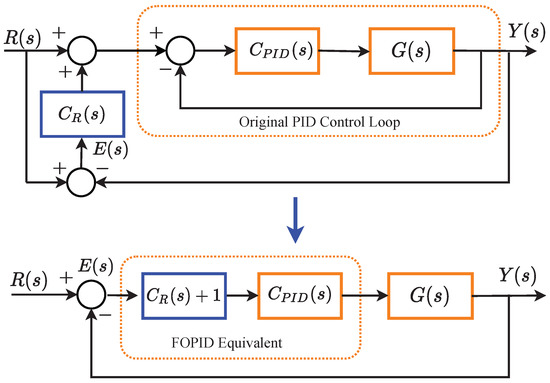
Figure 1.
Implementation of the retuning fractional-order proportional integral derivative (FOPID) system by using the PID control loop [9].
This method is of high industrial interest because it allows us to replace existing, suboptimally tuned PID control loops with optimally tuned PID or FOPID controllers essentially without interrupting the control process since the dynamics are introduced through manipulating the original reference signal. This means that the controlled process ideally does not experience any downtime and hence this change in control strategy should not result in additional expenses related to restarting the process after the change of controller has taken place.
As it can be seen from Figure 1, when discussing retuning control, in an ideal scenario one can just speak about the control loop consisting of a FOPID controller and plant in a negative unity feedback configuration because, at least from a purely theoretical perspective, the retuning method ensures that the complete control loop will indeed have the dynamics introduced by the external FOPID controller instead of those stemming from the original PID controller. In other words, it is equivalent to discussing a simpler FOPID control loop rather than the retuning control loop, at least for the sake of the simplicity of exposition.
2.2. Multi-Loop Mrac
Direct use of the MIT rule for control action brings out some instability concerns because the control action of the MIT rule is very sensitive to output amplitude of reference models [5]. This shortcoming is the main motivation for the development of two-loop MRAC-FOPID control structures, where an outer loop, which is an MRAC loop with MIT rule, only performs for adaptation to reference model.
The two-loop MRAC-FOPID control has been proposed to improve the robust control performance of the conventional FOPID control loop [8,9]. For this purpose, an additional outer loop to improve adaptation characteristics of the control system is appended to the FOPID control loop. In other words, the outer loop with a classical integer-order MIT rule encloses the inner loop and it is called the adaptation loop. This simplifies the design task of the outer loop. Thus, stability and set-point control performance are managed by the inner loop that is a FOPID control loop, and the disturbance rejection control to improve robust control performance is provided by the outer loop that is an MRAC loop with MIT rule. The design task of this control structure includes the following basic steps [8,9]:
Step 1: The inner loop (the FOPID control loop) is designed optimally by using any optimal FOPID tuning method. Robust stability and a satisfactory set-point control performance should be achieved by using a suitable optimal controller tuning method.
Step 2: A model of the inner loop is obtained and used as a reference model of MRAC structure.
Step 3: The outer loop is connected to the inner loop according to MIT rule.
The final structure of the two-loop MRAC-FOPID control is shown in Figure 2. In the figure, the adaptation gain is multiplied to the reference input r in order to shape the reference input when the response of the reference model diverges from the response of FOPID loop due to disturbance incidents. Therefore the outer loop, which is also known as the adaptation loop, enforces the inner loop, which is called the control loop, to behave similarly to the reference model that describes disturbance-free and optimal responses of the inner loop. Specifically, Step 2 ensures the correct establishment of this mechanism. It should be noted that in this work, Step 2 is modified. This will be clear from the following discussion. Specifically, the reference model is obtained independently from the inner loop.
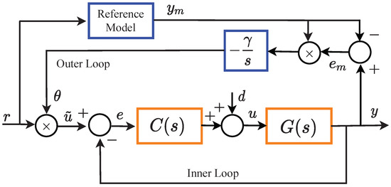
Figure 2.
Block diagram of multi-loop Model Reference Adaptive Control (MRAC)-FOPID system [9].
The closed-loop retuning FOPID control system was implemented and the FOPID controller was optimally tuned by using FOMCON toolbox [47].
The theoretical background of MIT rule to implement the outer loop was summarized as follows [8,9]:
The MIT rule works for the minimization of model error that is defined according to difference between outputs of inner loop (FOPID control loop) and the reference model as . Therefore, the error function to be minimized is written in form of square of instant model error
According to Figure 2, to perform adaptation by applying input-shaping technique, the input of closed-loop system is modified as , where the adaptation gain is determined according to the MIT rule. The MIT rule performs the continuous time gradient descent method to minimize the error function, it was expressed for MRAC [2,3,4,5,6] as
By considering multi-loop MRAC-FOPID structure in Figure 2, the model error can be expressed as [8,9]
Then, the sensitivity derivative is written by
where the transfer function represents the current model of the inner loop. When the reference input is substituted with in Equation (13), the sensitivity derivative can be obtained
By using the sensitivity derivative in Equation (11), MIT rule for the update of adaptation gain is obtained as
To investigate the contribution of the adaptation gain to system response, let us consider the response of the system in disturbance-free state and in case of a disturbance incident.
(i) Disturbance-free state: In this state, one can assume because reference model is configured as mathematical model of optimally tuned inner model. Accordingly, the adaptation gain can be written as,
In the disturbance-free state, outputs of reference model and the inner loop match each other, hence . When and conditions are used in Equation (12), one obtains . This arithmetically infers the state of because the reference model is non-zero function and the reference signal r is the independent input variable. Therefore, adaptation gain settles the value of in the disturbance-free state. It does not shape the reference input. This property validates that outer loop does not affect control performance of the inner loop in disturbance free case.
(ii) Disturbance state: In case of a disturbance incident, one can assume a perturbation of the system model due to additional dynamics of the additive interference of disturbance. This effect results in differentiation of inner loop model from the reference model, and let us assume . The MIT rule is based on gradient descent perform optimization of the adaptation gain to minimize error function and it leads to . Therefore, one can consider the case , where the adaptation should change to reach the state in time. When the MIT rule achieves the state , response of the reference model and response of the inner loop become the same, and impacts of disturbance incident at the system output are rejected by the change of .
This analysis reveals the fact that the performance of the multi-loop MRAC-FOPID control system depends on the capability of the reference model to represent the response of the closed-loop FOPID control system. Therefore, identifying an accurate model of the closed-loop FOPID control system is of vital importance. This requirement constitutes the central motivation of this study. Therefore, practical use of NARX modelling for multi-loop MRAC-FOPID control is tested in a relatively difficult control problem that is the disturbance rejection control of a nonlinear, unstable dynamical system, namely the ML system.
To address stability concerns related to this configuration, the relevant discussion is provided next. In particular, it is important to address to components of stability analysis: the theoretical one and the empirical one. In the former case, stability conditions are derived mathematically, in the latter one, experiments are conducted and the results analyzed to ensure that the control system is indeed stable.
Stability and convergence conditions of the multi-loop MRAC-FOPID control system was summarized as follows in [11]:
The reference model and inner loop are designed as a stable system. Therefore, a sufficient condition for stability of the multi-loop MRAC-FOPID control system can be written based on stability and convergence of model error . Assuming that the inner loop and reference model are designed stable, multi-loop MRAC-FOPID control systems are stable and convergent when model error is bounded, the input is bounded, and output is stable and convergent. Therefore, it is sufficient to investigate the convergence condition of model error to show the stability of multi-loop MRAC--FOPID control system.
Lemma 1.
(Zero condition of the model error [11]): For multi-loop MRAC-FOPID control structure, the model error takes a zero value () when the adaptation gain θ is equal to one and the transfer functions of reference model and inner loop are equal ().
Proof.
By considering the model error given by Equation (12) for multi-loop MRAC-FOPID control structure, the model error can be written for , and as
Then, the model error becomes zero. This proves a zero condition of the model error as to be and . □
Theorem 1.
(Stability of model error [11]): For a stable system models , multi-loop MRAC--FOPID control system is stable only if the model error function:
expresses a stable function.
Proof.
By using the adaptation rule of multi-loop MRAC-FOPID control system that was given by Equation (16) as , the model error can be derived as
Output of reference model can be written as . For a set-point control stability, one considers step response of the system. Therefore, the reference input is assumed to be a step function by substituting in Equation (19).
According to Lemma 1, a zero value of model error () is possible for the case of , and . By applying this condition, the model error is obtained as
The function is transfer function of inner loop that is a closed-loop FOPID controller. Therefore, it can be expressed in the form of . When is used in Equation (21), one can write and reach to Equation (18).
The multi-loop MRAC--FOPID control system is stable if the function given Equation (18) is a stable function (check if the all characteristic roots of characteristic equation of lies on the left half plane (LHP)). Then, one can infer that when function is LHP stable function, the amplitude is bounded. Since the reference model was always configured to be stable function in design, the reference model output is bounded ( ) and it leads output of plant is also bounded ( ), and whole system is stable. □
3. Mathematical Model of the Ml System: From a First Principles Model to a Narx Black Box Approximation
The content of the following section conveys the mathematical modeling of the ML system using two different approaches. First, first-principles modeling is considered; then, the NARX model is developed. It is important to compare the accuracy of both models to ensure that the latter represents a coherent model of the ML system’s dynamics.
The Magnetic Levitation System (MLS) is a nonlinear, open-loop unstable, time-varying dynamical system with negligible air friction force. Figure 3 shows a picture of an experimental ML setup that was used for testing the proposed control structure. The objective in this experimental system is to control the terminal voltage of an electromagnet so that the ferromagnetic sphere can be levitated at the desired distance from the magnet. One of the promising applications of ML is the ML transportation systems. Specifically, physically contactless transportation on a guide-way can offer a number of advantages such as lower noise, less friction forces, less costly maintenance, higher efficiency and less emission of exhaust fumes. These advantages make ML transportation a suitable candidate for future transportation possibilities [48,49]. For these reasons, robust control of the ML system introduces a significant control problem that has the potential of producing technological outcomes. Several works have addressed robust control performance of ML systems; for instance, fuzzy logic controllers [50] and FOPID controllers [9,17,51,52,53] were considered. It is important to stress that disturbance rejection and vibration control are essential problems in control of ML systems.
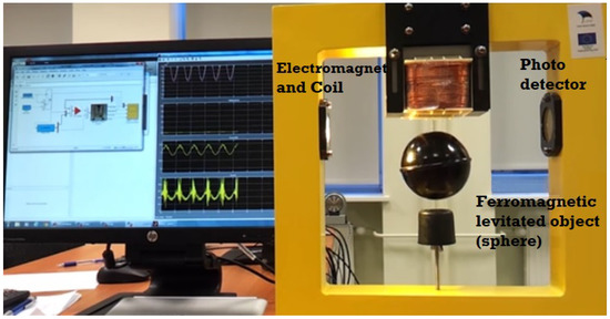
Figure 3.
Magnetic Levitation System (MLS) setup in A-Lab.
In order to compare among results including experimental and artificial models, the mathematical modeling of ML systems has been studied.
Magnetic levitator can be divided into two subsystems, mechanical and electrical [50,54]. For the electrical subsystem, it is important to single out electromagnetic coil inductance L (H), and its resistance, R (). The electrical subsystem can be described with the following well-known differential equation:
In order to determine the current in the coil, the resistor is connected in series with the coil. In that way, voltage can be measured across resistor , by using A/D convertor for measuring current i. Now, Equation (22) can be rewritten as:
After applying Laplace transform we obtain:
On the other side, modelling mechanical subsystem can be performed simply by defining force F, that represents the result of electromagnet activity to the ball:
where m is ball mass, g is gravitation constant, is magnetic force constant which is valid for pair electromagnet and ball, i is the current which flows through electromagnet, x is ball distance from magnet. Using second Newton’s law, Equation (25) can be rewritten as:
The value of electromagnetic coil current in steady state denoted as can be determined by Equation (26). This current defines a constant of ball position in a steady state case. If we take into consideration that velocity and acceleration are equal to zero in the state, then Equation (26) is given as:
Theoretically, regulation of the ball position can be performed by (27). However, external disturbances, uncertainty, system parameter variations, and high nonlinearity degree of the system require a feedback controller installation, which ensures stable control of these mechanical subsystems.
In general, adding linearity into the system must be done first, and after that control process begins. In this report, NARX neural network is used for experimental substitution of the real system of magnetic levitation. If the training process is successfully performed, we are going to get values on network outputs with minimal errors comparing to the output values of the real system. The nonlinear mathematical model of magnetic levitation system is given by the following equations [55]:
where , , are ball position, velocity and current respectively. u is the control signal. The corresponding parameters are given in Table 1.

Table 1.
Physical parameters of the ML system.
Variables and are limitations for current and voltage to avoid break down of device. In this paper, the mathematical output has been compared simultaneously with NN and experimental results during real-time experiments. It is important to have appropriate conversion tables which include the experimental measurement to convert between quantities in order to have accuracy in the simulation.
3.1. Nn-Narx Modeling of the Ml System
Nature successfully builds up biological neural systems to perform control and adaptation tasks of living beings effectively in their complicated conditions and dynamically changing environments. To benefit from these assets, ANNs, which resemble biological neural systems, are widely utilized in intelligent system design due to the benefits of the learning and prediction potential of ANN algorithms.
Autoregressive neural network models can learn responses of linear and nonlinear dynamical systems from sampled input and output data [21,24]. Therefore, these models can gain a significant flexibility for multi-loop MRAC-FOPID control structures to be easily employed in real-world applications. NARX modeling can automatically learn response of a wide-range of system models in black box form and this reduces the need for guessing the model structure prior to model identification. The reference model is automatically identified from data that are captured online from the input and output of controlled systems. This point is an important contribution of this study to transform the multi-loop MRAC-FOPID control structures into an intelligent control system and thus increase effectiveness of MRAC-FOPID control in practical nonlinear control applications. For experimental validation, the proposed control structure was employed for the control of a magnetic levitation system. The magnetic levitation control introduces a highly nonlinear, unstable system control problem.
The authors observed that the performance of multi-loop MRAC-FOPID control with the MIT rule largely depends on the capability of the reference model to represent the leading closed-loop dynamics of the experimental ML system. In [9], a linear model of the experimental ML system was used to obtain the transfer function of the closed-loop retuning FOPID control system. This linear function was used as the reference model. This modeling approach comes out with two drawbacks for multi-loop MRAC-FOPID control structure which was already mentioned. In the current study, to deal with these drawbacks, NARX modeling was employed to obtain a more accurate reference model. The use of neural networks in system identification allows utilization of machine learning techniques in control, and this enables the multi-loop MRAC-FOPID control structure with NARX model to be more adaptive and intelligent compared to previous configurations.
Artificial neural networks can be successfully applied in the modeling of complex nonlinear systems, systems with disturbances and insufficiently known parameters, unpredictable and uncoordinated systems [19,56]. Figure 4 shows a block diagram of the NARX model. It is composed of time delay blocks (TDL) and conventional artificial neuron models with input and loop weight coefficients (IW and LW, respectively), bias (b), and activation function (f). The vector is transmitted to the system as a two-layer input and is realized by passing a time delay block (b1) and in that way a part of Equation (33), is realized. The vector is obtained from the input weight coefficients defined in IW1,1, bias, b1, and the output network vector, , which leads to a time delay block and then multiplied by the weight coefficient, LW1,3. The resulting vector, is then directed to the first layer activation function, f1. The output from the first layer , which represents the result of the operation of the activation function, f1, reaches the second layer, which is converted to the vector by the weight coefficients of LW2,1 and the b2 bias. This vector is then plotted in bias f2 to obtain the final neural network output, y(t). The feedback from the output neurons to the input of network causes a system state formation and lead to mimicing dynamical system models. Therefore, it can learn and represent time responses of dynamic systems. Two-layer neural networks with a nonlinear activation function are capable of learning nonlinear relations in inputs and state transition patterns. This property enables representation of nonlinear system dynamics by NARX model when it is trained properly. Therefore, after training with input-output data of the dynamical systems, NARX model can mimic dynamical behavior of systems and it is employed for prediction of time response of dynamic systems. This property makes NARX modeling a good candidate solution for online modeling problems of nonlinear dynamical systems in intelligent control applications.
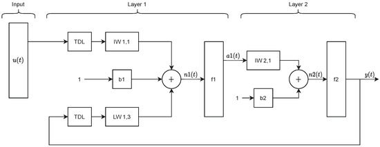
Figure 4.
Representation of neural network (NN)-nonlinear autoregressive neural network with external inputs (NARX) structure. The first layer activation function is generally a nonlinear activation function to model nonlinear relations in the data. The second layer activation function is a linear activation function that rescales NARX output to original output data. Thus, it can yield satisfactory predictions of a nonlinear system dynamics.
The reason why a neural network is selected for modeling is that neural networks are very good at time-series problems. A neural network with enough elements (neurons) can model dynamic systems with arbitrary accuracy. They are particularly well suited for addressing non-linear dynamic problems. Neural network is a good candidate for solving this problem. The network will be designed by using recordings of an actual levitated magnet’s position responding to a control current. The output of a NARX artificial neural network has the following form [20,23,24]:
where is the previous sample of NARX output and is the i-th previous sample of the NARX input. These samples are stored to the TDL buffers and the parameter n configures the buffer size that determines depth of delayed memory to be considered in the NARX model. The feedback from model output with previous values [, , ,..,] forms an autoregressive model to predict the current value of the dynamical system. This delayed output values constitute pseudo-states to allow learning of system dynamics from time response data. The weight coefficients are indicated by , obtained vector is stated with n, first layer named , b is bias, and f is activation functions.
To obtain a black-box model of the experimental ML system via NARX modeling, time-series data was collected from the output of controller and the sphere position sensors. The data from output of controller was used for input data () of NARX model. A time-series signal for the sphere position was collected and used to form output data () of NARX model. The data set [] consists of 30,001 samples and it was used for training of the NARX model. The sampling period of data collection was 0.001 s and the data collection interval was continued for 30 s.
In this section, the real MLS system is presented in order to compare the simulated models. The real MLS model is located between two ADC cards as the hardware-in-the-loop part. Details of neural network is shown in Table 2. The NARX model used a one input and three output neural network with a input layer with 12 neurons and hidden layer with one neuron. The buffer size (n) set to 1, which provides a sample delaying of input and output data in TDL blocks. Figure 5 shows the input and output with filters. The reason for using the filter is that in the real model, the signal has noise and needs a filter. The same was done in the neural network model. In fact, the neural network model is the same as the maglev model with a raw signal without a filter.
Table 2.
The parameters of the neural network.
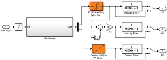
Figure 5.
Neural network model with ML’s filter.
After sending the simulated control signal to the hardware and acquiring the real signals (voltage) from the hardware, the signals are converted to corresponding position, [m] and current [A] by experimental look-up tables. Then, the signals are filtered to eliminate undesirable noises. The velocity of the ball is obtained by an inaccurate, but acceptable, memory element which applies a unity integration step delay. The output is the previous input value. In Figure 6, an overview of our project is shown. The mathematical model and ANN model were inserted in the real-time Simulink model in order to compare the three parts in the same situations. The input includes the range of sine wave, chirp wave with the frequency variation from 1 Hz to 6 Hz, the step input which contains all range of frequency and the constant input (steady state position is 0.011 m).
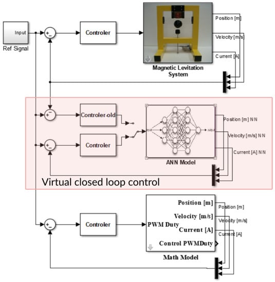
Figure 6.
Overview of three parts, hardware, ANN model and Mathematical model.
To determine this NARX configuration, several sizes of TDL and neuron numbers in the hidden layer were tested for data from the experimental system. The best modeling performance was obtained for 12 neurons in hidden layer and TDL units with one sample delay element.
The training algorithm used was the Levenberg–Marquardt method and the training process was completed in 113 iterations. The training task of the NARX model was carried out off-line by using the data set [] that was collected from the experimental system. The time-series data set was automatically divided into training, validation and test sets. Figure 6 shows a Simulink model that was developed for the training of NARX model in a virtual closed-loop. For the closed-loop model identification, NARX model is put into a virtual control loop that is composed of the controller function of the identified closed-loop system and the NARX model to access the in-loop dynamics of the ML system. This virtual closed-loop can provide relevant training data, which is related to the in-loop dynamics of ML setup, to learn by NARX model. In the cases that outputs of the identified closed-loop experimental control system and the virtual closed-loop system with NARX model match, NARX model is said to be learned responses of ML system in the closed-loop. In the following section, this virtual closed-loop control system with NARX model is used as the reference model of multi-loop MRAC-FOPID control structure.
All simulation results were obtained at Control Systems Research Laboratory, Tallinn University of Technology.
3.2. Off-Line Results
In this section, the trained ANN has been simulated. The output of the controller was saved and used for off-line simulation. Figure 7 represents the levitation characteristics (input control voltage and output position). Ball position of real system and ANN model are shown. The steady state position for real model is 0.01085 m. It is clearly shown that the ANN model tracks the input in steady state position, (0.0109 m) with about 0.5% error. However, in the transient regions there is considerable offset of about 7% error.
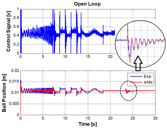
Figure 7.
Input and output signals to train the NARX model for closed-loop model identification.
Figure 7 includes data when the ball is hit to create an external disturbance. The reason ANN response is seen in the present of disturbance is that the input of ANN (control output) is the same as real-model input. However, it is not realistic and the individual control output is used to control the ANN model in the real life experiment. The approximation of error in this noteworthy experiment gives mean square error (MSE) equal to . The duration time of simulation is 30 s. The MSE is calculated as sum of difference between the samples of real ball position and ANN ball position dividing by number of samples (30,001 samples).
3.3. Real-Life Results
In this section, the whole system, including the mathematical model, ANN model, and real-time MLS, is simulated simultaneously. Since the system is fundamentally unstable, it means using the closed-loop system is essential. The input signals, including chirp, step, sinand constant source, are applied and used for three models. The control signal is generated by LQ controller and converted to PWM in real MLS.
The output of the ANN model is based on real-time controller. On the other hand, the controller already has been designed for real-time model. However, the obtained ANN is using the control signal that is being generated by real-model. The ANN model is not exactly like the real-model. It means a new model may need to implement a new controller in the simulation. Since the MLS is a highly nonlinear unstable system, it needs to illustrate complex control algorithms. The obtained ANN model can control itself by previous controller with minor changes if it works in linear region. The developed controller is applied to the system. The results are shown from Figure 8 and Figure 9. In Figure 8, it is seen that the ball is exposed to disturbance in real life, that is why the simulation models can not respond to real life disturbance.
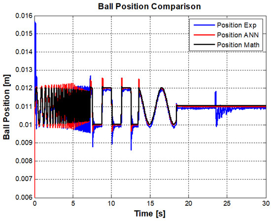
Figure 8.
Ball position comparison among real model, ANN model and Mathematical model.
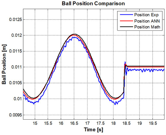
Figure 9.
A comparison of ANN model performance and mathematical model performance.
The figures show the higher frequency response of three models up to 7 s. It can be seen that the position response in real model is less than that of the mathematical and ANN models. In other words, the bandwidth of mathematical model is more than real-model. However, the ANN result indicates better behavior in high frequency.
In Figure 9, it can be seen that the transient response is compensated desirably and the steady state response of the ANN model is acceptable. However, for a high frequency region like chirp signal or step points in pulse signals performance has not been achieved well. The MSE error, in this case has been decreased considerably compared to the off-line ANN model.
In this paper, NN-NARX structure and linearization by dynamic output feedback were implemented to control ball position of a real magnet levitation system. The noisy signals (signals before filters) are used in order to train the neural network model more accurately. The Levenberg–Marquardt method gives the best results with 12 neurons in the hidden layer and one delay. The training process achieved best performances after 113 iterations. Increasing the number of neurons in the hidden layer in this project did not improve the accuracy of the model. As the input signal in closed-loop system depends on the error between input and its output, the ANN controller is developed instead of real MLS LQ controller. Results indicate the steady state and transient response is compensated desirably for the neural network model.
For the purpose of comparing all models, the mean square error between the input command and output of models was calculated. Table 3 shows the results where YEXP, YANN, and YMATH represent the ball position in the experiment, artificial neural network, and mathematical model, respectively. UEXP is the input command in the experimental test. Based on results in the figures cited above and Table 3, it is concluded that the identified model has acceptable performance.
Table 3.
MSE ball position comparison among models.
4. Multi-Loop Mrac-Fopid Control with Narx Reference Model for Ml System Control Application
This section presents the experimental results of multi-loop MRAC-FOPID control of ML system by using a NARX reference model. The design steps of Multi-loop MRAC-FOPID control was carried out for experimental ML system:
- i.
- The closed-loop retuning FOPID control system was implemented and FOPID controller was optimally tuned by using FOMCON toolbox [47].
- ii.
- The control signal and sphere position data from the designed closed-loop control system described above were collected and these data were used to train the NARX model in the virtual closed-loop control system. Thus, the virtual closed-loop PID control loop with the NARX model is used as reference model to represent closed-loop retuning FOPID control system.
- iii.
- The outer loop is connected to inner loop according to MIT rule as shown in Figure 10.
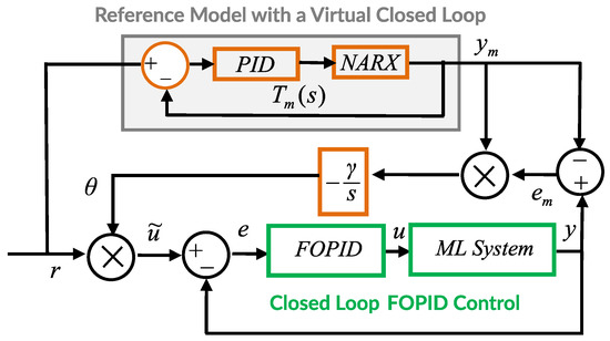 Figure 10. Block diagram of multi-loop MRAC-FOPID control with a NARX reference model.
Regarding the configuration of the experimental system, in Figure 11, the complete control diagram used to implement both simulation and real time experiments is presented. For the implementation of the experimental configuration, the MATLAB/Simulink environment is used with FOMCON toolbox for implementing fractional-order control. The tuning of the controllers used in the retuning loop is detailed in [9]. However, compared to that work, the value of in the MRAC loop was tuned down from to in order to minimize high frequency components entering the control system and causing excessive vibrations of the sphere.
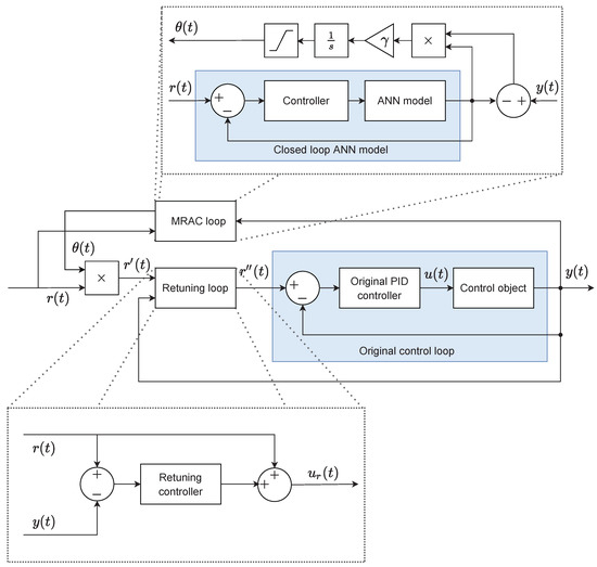
Figure 11.
Complete experimental configuration for evaluating the multi-loop control structure. There are three control loops in total: the original PID control loop with reference input , the retuning loop with reference input that replaces the dynamics of the original loop with those of the optimally tuned FOPID controller, and the MRAC loop to which the original reference input is connected. By bypassing reference inputs in various ways, it is possible to achieve different simulation scenarios with the MRAC loop and retuning control loop enabled or disabled independently. This schematic diagram serves as the basis for both pure software simulations and real-time experiments in MATLAB/Simulink software.
Figure 12 shows a simulation result to demonstrate disturbance rejection performance of multi-loop MRAC-FOPID with NARX model. After settling of the sphere to a height of 0.0109 m, a step-down disturbance and then step-up input disturbances were applied at the simulation times 10 s and 40 s, respectively. The responses of the proposed multi-loop MRAC-FOPID and the conventional FOPID control are shown in the figure. The conventional FOPID control is the inner loop that was performed by disabling contribution of outer loop (MRAC with MIT rule). Thus we can test control improvements of the multi-loop MRAC-FOPID with the NARX model compared to the FOPID control loop alone. At disturbance incidents, multi-loop MRAC-FOPID with NARX model settles back to the set-point faster with lower ripples. These results indicate considerable improvements indisturbance rejection control performance of the FOPID control loop when the outer loop (MRAC) is enabled.
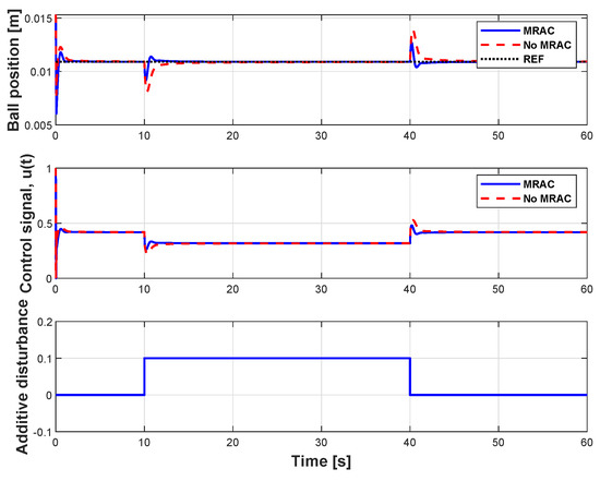
Figure 12.
Disturbance responses of the multi-loop MRAC-FOPID control with NARX reference model and the FOPID control loop (When MRAC is disabled).
Armed with promising simulation results, real-time verification of the multi-loop control system was performed. The Simulink model was built according to Figure 11 with additive disturbance injected into the system using the control input in the original PID control loop. The model runs on a Desktop PC (3.40 GHz Processor and 8.00 GB RAM) and the computational complexity of the control scheme allows real-time operation with 0.001 data sampling rate. Figure 13 and Figure 14 show experimental results to demonstrate disturbance rejection performance of the multi-loop MRAC-FOPID control with NARX reference in comparison with the conventional FOPID control (MRAC is disabled). In Figure 13, after settling to the set-point of 0.0109 m high, a step-down input disturbance signal was applied at 10 s. Responses of control systems to this disturbance signal are compared in the figure. The multi-loop MRAC-FOPID control improves disturbance responses of ML system with faster resettling and lower ripples around the set-point. Figure 14 shows impacts of a continuous input disturbance in the form of sinusoidal waveform on the set-point control performance. The sinusoidal disturbance with roughly 7 s periods was applied. The experimental results show that the multi-loop MRAC-FOPID control with NARX reference modeling better suppresses the sinusoidal disturbance at the system output compared the FOPID control loop. These two tests evidently verify contribution of outer loop (adaptation loop) to disturbance rejection performance of the inner loop (control loop). Results also validate the improvement of disturbance rejection control capacity without any deterioration of set-point control performance. The results are also summarized in Table 4. This property is a natural result of designing loops with specialized objectives in multi-loop structure. This control structure can be a feasible solution of the tradeoff between set-point and disturbance rejection performances of single loop systems.
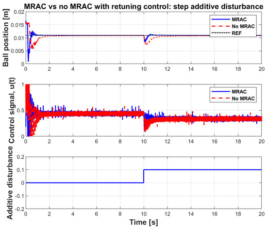
Figure 13.
Step disturbance responses of the multi-loop MRAC-FOPID control with NARX reference model and the FOPID control loop (When MRAC is disabled).
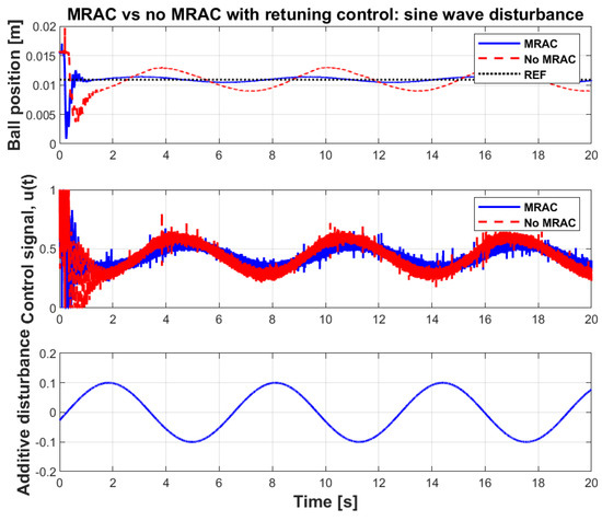
Figure 14.
Sinusoidal disturbance responses of the multi-loop MRAC-FOPID control with NARX reference model and the FOPID control loop (When MRAC is disabled).
Table 4.
Comparison of experimental performances of control systems with the MRAC loop disabled and enabled.
In addition, experiments involving the original PID control loop with MRAC adaptation loop were performed in the same way, i.e., for two different types of disturbance and with MRAC loop enabled and disabled. The results of the successful experiments are presented in Figure 15 and Figure 16 and also in Table 4. Only those experiments that had the MRAC loop enabled were successful, so only those are presented. In other cases, the control loop failed to levitate the sphere and keep it in a steady state—in the real experiment the sphere was simply thrown out from the working area due to unstable behavior of the control system. The original PID control loop only works in the case when the sphere is manually placed in the magnetic field away from the rest, whereas other types of control configurations are also able to successfully levitate the sphere from its initial position on the rest. Taking the results into account, one can see that even with the MRAC loop enabled, the original PID control loop although capable of levitating the sphere, still shows inferior performance compared to the fractional retuning control with the MRAC loop enabled.
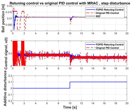
Figure 15.
Step disturbance responses of the MRAC system with the original PID control loop.
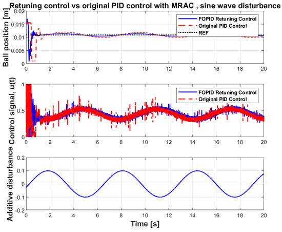
Figure 16.
Sine wave disturbance responses of MRAC system with original PID control loop.
5. Conclusions and Discussion
This experimental study investigated the use of multi-loop MRAC-FOPID control with NARX reference modeling in the disturbance rejection control problem of ML systems. Simulation and experimental studies were conducted and it was observed that NARX reference modeling enables more intelligent realization of multi-loop MRAC-FOPID control structures. Simulation and experimental studies reveal that NARX modeling can be utilized for online modeling of nonlinear, unstable dynamical systems and it can be a feasible solution for real-time modeling requirements of intelligent control systems. This study also shows that the recurrent artificial neural network serves for improvement of classical control loops.
It is remarkable that in this study, three major components were considered, which can be used independently to formulate a robust and well-performing control system: (1) the NARX-based control loop with a PID controller that was tuned separately from the FOPID control in the main loop that can be used as an accurate reference model of the controlled process; (2) the retuning FOPID control which replaces the dynamics of another existing PID controller; (3) the MRAC loop which together with the reference model results in improved disturbance rejection in the overall control loop.
Indeed, the resulting multi-loop MRAC-FOPID control with NARX reference modeling combines robust stability and set-point control performance of the FOPID control loop with adaptation skills of MRAC loop. Disturbance rejection control is a major concern for practical control applications. To maintain optimal control performance in real-world application, disturbance rejection control performance should be improved in addition to set-point and stability performance. The multi-objective control structures with specialized loops can provide more robust control performance than single control loops in real-world applications. Moreover, this multi-loop control structure can be easily applied to existing closed-loop control systems and this can give an opportunity to upgrade existing classic control loops to multi-loop MRAC loops without changing any parameter or any block of the existing control loops. The NARX reference model facilitates this upgrade process by performing real-time closed-loop model identification of the system and makes the multi-loop MRAC-FOPID control structure more adaptive and intelligent by providing it with benefits stemming from contemporary machine learning.
The MIT rule presents a shortcoming of being sensitive to output amplitude of the reference input [5,11]. Very high amplitudes may cause instability of the system [5] and very low amplitudes diminish effectiveness of MIT rule to respond disturbances [11]. In [11], several alternative multi-loop control structures have been suggested to deal with these drawbacks. Future work can be planned for practical realization and performance evaluations of multi-loop control structure with NARX reference modeling.
Author Contributions
Conceptualization, A.T., E.P., K.V. and H.A.; methodology A.T., E.P., K.V, and B.B.A.; validation, H.A. and A.T.; writing—original draft preparation, A.T., B.B.A. and H.A.; writing—review and editing, E.P. and K.V; supervision, A.T. and E.P. All authors have read and agreed to the published version of the manuscript.
Funding
The work was supported by the Estonian Research Council grant PRG658.
Conflicts of Interest
The authors declare no conflict of interest. The funders had no role in the design of the study; in the collection, analyses, or interpretation of data; in the writing of the manuscript, or in the decision to publish the results.
References
- Alagoz, B.B.; Deniz, F.N.; Keles, C.; Tan, N. Implicit disturbance rejection performance analysis of closed loop control systems according to communication channel limitations. IET Control Theory Appl. 2015, 9, 2522–2531. [Google Scholar] [CrossRef]
- Butler, H. Proceedings of the Model Reference Adaptive Control: From Theory to Practice; Prentice Hall International Series in Systems and Control Engineering; Prentice Hall: Upper Saddle River, NJ, USA, 1992. [Google Scholar]
- Vinagre, B.; Petráš, I.; Podlubny, I.; Chen, Y. Using fractional order adjustment rules and fractional order reference models in model-reference adaptive control. Nonlinear Dyn. 2002, 29, 269–279. [Google Scholar] [CrossRef]
- Lavretsky, E. Adaptive control: Introduction, overview, and applications. In Proceedings of the NASA Adaptive Control Workshop, NASA Marshall Space Center, Huntsville, AL, USA, 24 February 2009. [Google Scholar]
- Jain, P.; Nigam, M. Design of a Model Reference Adaptive Controller Using Modified MIT Rule for a Second Order System. Adv. Electron. Electr. Eng. 2013, 3, 477–484. [Google Scholar]
- Swamkar, P.; Nema, R.; Swarnkar, P.; Kumar, J.; Nema, R. Comparative Analysis of MIT Rule and Lyapunov Rule in Model Reference Adaptive Control Scheme. Innov. Syst. Des. Eng. 2011, 2, 154–162. [Google Scholar]
- Kavuran, G.; Ates, A.; Alagoz, B.B.; Yeroglu, C. An experimental study on model reference adaptive control of TRMS by error-modified fractional order MIT rule. Control Eng. Appl. Inform. 2017, 19, 101–111. [Google Scholar]
- Alagoz, B.B.; Tepljakov, A.; Petlenkov, E.; Yeroglu, C. Multi-Loop model reference adaptive control of fractional-order PID control systems. In Proceedings of the 2017 IEEE 40th International Conference on Telecommunications and Signal Processing (TSP), Barcelona, Spain, 5–7 July 2017. [Google Scholar] [CrossRef]
- Tepljakov, A.; Alagoz, B.B.; Gonzalez, E.; Petlenkov, E.; Yeroglu, C. Model Reference Adaptive Control Scheme for Retuning Method-Based Fractional-Order PID Control with Disturbance Rejection Applied to Closed-Loop Control of a Magnetic Levitation System. J. Circuits Syst. Comput. 2018, 27. [Google Scholar] [CrossRef]
- Rajesh, R.; Deepa, S. Design of direct MRAC augmented with 2 DoF PIDD controller: An application to speed control of a servo plant. J. King Saud Univ. Eng. Sci. 2020, 32, 310–320. [Google Scholar] [CrossRef]
- Alagoz, B.B.; Tepljakov, A.; Petlenkov, E.; Yeroglu, C. Multi-Loop Model Reference Proportional Integral Derivative Controls: Design and Performance Evaluations. Algorithms 2020, 13, 38. [Google Scholar] [CrossRef]
- Chen, Y.; Petras, I.; Xue, D. Fractional order control-a tutorial. In Proceedings of the 2009 IEEE American Control Conference, St. Louis, MO, USA, 10–12 June 2009. [Google Scholar] [CrossRef]
- Monje, C.A.; Chen, Y.; Vinagre, B.M.; Xue, D.; Feliu, V. Fractional-Order Systems and Controls; Springer: London, UK, 2010. [Google Scholar] [CrossRef]
- Podlubny, I. Fractional Differential Equations; Mathematics in Science and Engineering; Academic Press: San Diego, CA, USA, 1999. [Google Scholar]
- Zhao, C.; Xue, D.; Chen, Y.Q. A fractional order PID tuning algorithm for a class of fractional order plants. In Proceedings of the IEEE International Conference Mechatronics and Automation, Niagara Falls, ON, Canada, 29 July–1 August 2005; Volume 1, pp. 216–221. [Google Scholar] [CrossRef]
- Padula, F.; Visioli, A. Advances in Robust Fractional Control; Springer: Cham, Switzerland, 2014. [Google Scholar]
- Tepljakov, A.; Petlenkov, E.; Belikov, J.; Gonzalez, E.A. Design of retuning fractional PID controllers for a closed-loop magnetic levitation control system. In Proceedings of the 2014 13th International Conference on Control, Automation, Robotics & Vision, ICARCV, Singapore, 10–12 December 2014; pp. 1345–1350. [Google Scholar]
- Tepljakov, A.; Gonzalez, E.A.; Petlenkov, E.; Belikov, J.; Monje, C.A.; Petráš, I. Incorporation of fractional-order dynamics into an existing PI/PID DC motor control loop. ISA Trans. 2016, 60, 262–273. [Google Scholar] [CrossRef]
- Trisanto, A. PID controllers using neural network for multi-input multioutput magnetic levitation system. Electrician 2007, 1, 62–68. [Google Scholar]
- Vassiljeva, K.; Tepljakov, A.; Petlenkov, E. NN-ANARX model based control of liquid level using visual feedback. In Proceedings of the 2015 IEEE 13th International Conference on Industrial Informatics (INDIN), Cambridge, UK, 22–24 July 2015. [Google Scholar] [CrossRef]
- Jiang, Y.; Yang, N.; Yao, Q.; Wu, Z.; Jin, W. Real-time moisture control in sintering process using offline–online NARX neural networks. Neurocomputing 2020, 396, 209–215. [Google Scholar] [CrossRef]
- Abouelazayem, S.; Glavinić, I.; Wondrak, T.; Hlava, J. Adaptive Control of Meniscus Velocity in Continuous Caster based on NARX Neural Network Model. IFAC-PapersOnLine 2019, 52, 222–227. [Google Scholar] [CrossRef]
- Petlenkov, E.; Nomm, S.; Kotta, U. Neural Networks Based ANARX Structure for Identification and Model Based Control. In Proceedings of the 2006 IEEE 9th International Conference on Control, Automation, Robotics and Vision, Singapore, 5–8 December 2006. [Google Scholar] [CrossRef]
- Antić, D.; Milovanović, M.; Nikolić, S.; Milojković, M.; Perić, S. Simulation Model of Magnetic Levitation Based on NARX Neural Networks. Int. J. Intell. Syst. Appl. 2013, 5, 25–32. [Google Scholar] [CrossRef][Green Version]
- Kumpati, S.N.; Kannan, P. Identification and control of dynamical systems using neural networks. IEEE Trans. Neural Netw. 1990, 1, 4–27. [Google Scholar]
- Hagan, M.T.; Demuth, H.B. Neural Networks for Control. In Proceedings of the 1999 American Control Conference, Hyatt Regency, San Diego, San Diego, CA, USA, 2–4 June 1999; pp. 1642–1656. [Google Scholar]
- Slotine, J.J.E.; Li, W. Applied Nonlinear Control; Prentice Hall: Englewood Cliffs, NJ, USA, 1991; Volume 199. [Google Scholar]
- Spooner, J.T.; Maggiore, M.; Ordonez, R.; Passino, K.M. Stable Adaptive Control and Estimation for Nonlinear Systems: Neural and Fuzzy Approximator Techniques; John Wiley & Sons: Hoboken, NJ, USA, 2004; Volume 43. [Google Scholar]
- Fatemimoghadam, A.; Toshani, H.; Manthouri, M. Control of magnetic levitation system using recurrent neural network-based adaptive optimal backstepping strategy. Trans. Inst. Meas. Control 2020, 0142331220911821. [Google Scholar] [CrossRef]
- Hajimani, M.; Gholami, M.; Dashti, Z.A.S.; Jafari, M.; Shoorehdeli, M.A. Neural adaptive controller for magnetic levitation system. In Proceedings of the 2014 IEEE Iranian Conference on Intelligent Systems (ICIS), Bam, Iran, 4–6 February 2014; pp. 1–6. [Google Scholar]
- Bidikli, B. An observer-based adaptive control design for the maglev system. Trans. Inst. Meas. Control. 2020, 0142331220932396. [Google Scholar] [CrossRef]
- Zhang, J.; Wang, X.; Shao, X. Design and real-time implementation of Takagi–Sugeno fuzzy controller for magnetic levitation ball system. IEEE Access 2020, 8, 38221–38228. [Google Scholar] [CrossRef]
- Ladaci, S.; Charef, A. On fractional adaptive control. Nonlinear Dyn. 2006, 43, 365–378. [Google Scholar] [CrossRef]
- Wei, Y.; Sun, Z.; Hu, Y.; Wang, Y. On fractional order composite model reference adaptive control. Int. J. Syst. Sci. 2016, 47, 2521–2531. [Google Scholar] [CrossRef]
- Aguila-Camacho, N.; Duarte-Mermoud, M.A. Fractional adaptive control for an automatic voltage regulator. ISA Trans. 2013, 52, 807–815. [Google Scholar] [CrossRef]
- Keziz, B.; Ladaci, S.; Djouambi, A. Design of a MRAC-Based Fractional order PI λ D μ Regulator for DC Motor Speed Control. In Proceedings of the 3rd International Conference on Electrical Sciences and Technologies in Maghreb (CISTEM 2018), Algiers, Algeria, 28–31 October 2018; pp. 1–6. [Google Scholar]
- Hartley, T.T.; Lorenzo, C.F. Dynamics and Control of Initialized Fractional-Order Systems. Nonlinear Dyn. 2002, 29, 201–233. [Google Scholar] [CrossRef]
- Vinagre, B.M.; Podlubny, I.; Hernández, A.; Feliu, V. Some Approximations Of Fractional Order Operators Used In Control Theory And Applications. Fract. Calc. Appl. Anal. 2000, 3, 945–950. [Google Scholar]
- Matignon, D. Stability Results For Fractional Differential Equations With Applications To Control Processing. Comput. Eng. Syst. Appl. 1997, 2, 963–968. [Google Scholar]
- Radwan, A.; Soliman, A.; Elwakil, A.; Sedeek, A. On the stability of linear systems with fractional-order elements. Chaos Solitons Fractals 2009, 40, 2317–2328. [Google Scholar] [CrossRef]
- Senol, B.; Ates, A.; Baykant Alagoz, B.; Yeroglu, C. A numerical investigation for robust stability of fractional-order uncertain systems. ISA Trans. 2014, 53, 189–198. [Google Scholar] [CrossRef] [PubMed]
- Alagoz, B.B. Hurwitz stability analysis of fractional order LTI systems according to principal characteristic equations. ISA Trans. 2017, 70, 7–15. [Google Scholar] [CrossRef]
- Chen, Y.; Vinagre, B.M.; Podlubny, I. Continued Fraction Expansion Approaches to Discretizing Fractional Order Derivatives?an Expository Review. Nonlinear Dyn. 2004, 38, 155–170. [Google Scholar] [CrossRef]
- Oustaloup, A.; Levron, F.; Mathieu, B.; Nanot, F. Frequency-band complex noninteger differentiator: Characterization and synthesis. IEEE Trans. Circuits Syst. Fundam. Theory Appl. 2000, 47, 25–39. [Google Scholar] [CrossRef]
- Deniz, F.N.; Alagoz, B.B.; Tan, N.; Koseoglu, M. Revisiting four approximation methods for fractional order transfer function implementations: Stability preservation, time and frequency response matching analyses. Annu. Rev. Control 2020, 49, 239–257. [Google Scholar] [CrossRef]
- Tepljakov, A. Implementation of Fractional-Order Models and Controllers. In Fractional-order Modeling and Control of Dynamic Systems; Springer International Publishing: Berlin/Heidelberg, Germany, 2017; pp. 77–105. [Google Scholar] [CrossRef]
- Tepljakov, A.; Petlenkov, E.; Belikov, J. FOMCON toolbox for modeling, design and implementation of fractional-order control systems. In Applications in Control; Petráš, I., Ed.; De Gruyter: Berlin, Germany, 2019; pp. 211–236. [Google Scholar] [CrossRef]
- bo Zhou, H.; an Duan, J. Levitation mechanism modelling for maglev transportation system. J. Cent. South Univ. Technol. 2010, 17, 1230–1237. [Google Scholar] [CrossRef]
- Yan, L. Development and Application of the Maglev Transportation System. IEEE Trans. Appl. Supercond. 2008, 18, 92–99. [Google Scholar] [CrossRef]
- Dragos, C.A.; Preitl, S.; Precup, R.E.; Bulzan, R.G.; Petriu, E.M.; Tar, J.K. Experiments in fuzzy control of a Magnetic Levitation System laboratory equipment. In Proceedings of the IEEE 8th International Symposium on Intelligent Systems and Informatics, Subotica, Serbia, 10–11 September 2010. [Google Scholar] [CrossRef]
- Gole, H.; Barve, P.; Kesarkar, A.A.; Selvaganesan, N. Investigation of fractional control performance for magnetic levitation experimental set-up. In Proceedings of the 2012 IEEE International Conference on Emerging Trends in Science, Engineering and Technology (INCOSET), Tiruchirappalli, India, 13–14 December 2012. [Google Scholar] [CrossRef]
- Yu, P.; Li, J.; Li, J. The Active Fractional Order Control for Maglev Suspension System. Math. Probl. Eng. 2015, 2015, 1–8. [Google Scholar] [CrossRef]
- Muresan, C.I.; Ionescu, C.; Folea, S.; Keyser, R.D. Fractional order control of unstable processes: The magnetic levitation study case. Nonlinear Dyn. 2014, 80, 1761–1772. [Google Scholar] [CrossRef]
- Dolga, V.; Dolga, L. Modeling and simulation of a magnetic levitation system. Ann. Oradea. Univ. Fascicle Manag. Technol. Eng. 2007, 6, 16. [Google Scholar]
- Inteco Sp. z o.o. INTECO Official Webpage. Available online: http://www.inteco.com.pl/ (accessed on 13 July 2015).
- Rafiq, M.Y.; Bugmann, G.; Easterbrook, D.J. Neural network design for engineering applications. Comput. Struct. 2001, 79, 1541–1552. [Google Scholar] [CrossRef]


© 2020 by the authors. Licensee MDPI, Basel, Switzerland. This article is an open access article distributed under the terms and conditions of the Creative Commons Attribution (CC BY) license (http://creativecommons.org/licenses/by/4.0/).