Two-Component Bayesian Hierarchical Models for Cost-Benefit Analysis of Traffic Barrier Crash Count

Abstract

Road departure crashes tend to be hazardous, especially in rural areas like Wyoming. Traffic barriers could be installed to mitigate the severity of those crashes. However, the severity of traffic barriers crashes still persists. Besides various drivers and environmental characteristics, the roadways and barrier geometric characteristics play a critical role in the severity of barrier crashes. The Wyoming department of transportation (WYDOT) has initiated a project to identify and optimize the heights of those barriers that are below the design standard, while prioritizing them based on the monetary benefit. This is to optimize first barriers that need an immediate attention, considering the limited budget, and then all other barriers being under design. In order to account for both aspects of frequency and severity of crashes, equivalent property damage only (EPDO) was considered. The data of this type besides having an over-dispersion, exhibits excess amounts of zeroes. Thus, a two-component model was employed to provide a flexible way of addressing this problem. Beside this technique, one-component hierarchical modeling approach was considered for a comparison purpose. This paper presents an empirical cost-benefit analysis based on Bayesian hierarchical machine learning techniques. After identifying the best model in terms of the performance, deviance information criterion (DIC), the results were converted into an equation, and the equation was used for a purpose of machine learning technique. An automated method generated cost based on barriers’ current conditions, and then based on optimized barrier heights. The empirical analysis showed that cost-sensitive modeling and machine learning technique deployment could be used as an effective way for cost-benefit analysis. That could be achieved through measuring the associated costs of barriers’ enhancements, added benefits over years and consequently, barrier prioritization due to lack of available budget. A comprehensive discussion across the two-component models, zero-inflated and hurdle, is included in the manuscript.

1. Introduction

Crashes are rare, but their occurrence can have devastating impact on the passengers of vehicles. These crashes are one of the leading causes of high number of deaths worldwide, with more than a million deaths and about 50 million severe injuries annually [1]. Run off the road (ROTR) accounts for a significant proportion of the high number of fatalities. Traffic barriers could be installed with the objective of reducing the severity of ROTR crashes. However, the severity of those crashes still persists; in fact, traffic barrier crashes are identified as the third most common causes of fixed-object fatalities, after trees and the utility poles [2].

Beside various environmental and driver characteristics contributing to the severity of barrier crashes, the geometric characteristics of these barriers are one of the main causes of the death. For instance, a barrier height above the recommended range could result in an underride crash, while override could be expected for the short barriers. In Wyoming, there is a significant number of old barriers which do not satisfy current height standards. Upgrading these barriers to the appropriate height will require much resources over several years.

It is therefore essential to develop a process for optimizing and upgrading barriers. Thus, the Wyoming department of transportation (WYDOT) has initiated a project to measure all the barriers’ geometric characteristics in the state. More than a million linear feet of barriers geometric and roadside characteristics were collected and measured. The collected data would not only help to enhance the below-design barriers, but also to identify the relationship between crash severity and the barriers geometric characteristics through conducting a statistical analysis. In addition, due to limited budget, the project needs to identify which barriers’ upgrades would result in higher benefits. The developed prioritization process will facilitate the gradual upgrade of barriers based on available annual budgets.

In order to provide a prioritization process, monetary evaluation of barrier enhancement was conducted with a help of machine learning technique. The technique was used to inform the policy makers about how much money they could expect to gain after optimizing barriers. To fulfill the aforementioned points, several steps are worthy of mention, as follows:

• Both state highway and interstate systems were aggregated in this study. However, to account for variation in response across these two-highway systems, a dummy variable of highway type was incorporated in the analysis.
• Various barriers were considered in this study. However, in order to account for similar characteristics, correlation across same traffic barrier types or heterogeneity resulted from the effects of various barrier types on crash observation, the hierarchical framework was employed.
• In order to account for the exposures, various variables such as barrier length and traffic were incorporated in the analysis.
• After a model is trained across all barriers in the highway and interstate systems, the trained model was implemented only on those barriers that are below/above recommended heights.
• Barrier cost with no enhancement: the trained model was implemented on the current data for 10 years with only traffic as a varied variable during 10-year period: this evaluates how much money due to crashes is expected if barriers are not optimized.
• Barriers cost with barrier height enhancement: the barriers were enhanced to their optimal values based on the recommended height in the literature review. The trained model was then implemented again over 10 years, while traffic was increased at a constant rate.
• The cost of barriers enhancement was considered in the cost-benefit analysis when barriers were enhanced, and added to the total cost of 6.
• As the analysis was based on equivalent property damage only (EPDO), this factor is converted to its monetary value so that the barrier enhancement cost could be added to the EPDO cost.
• The barriers were ranked based on expected benefit so that WYDOT could first enhance those barriers with more benefits.
• A main challenge of modeling barriers EPDO was sparsity and excess number of zeroes in the dataset, which was addressed by a two-component model.

Most of the studies in the literature review either focused on the severity [3] or the frequency of barrier crashes [4]. However, not many studies have considered both aspects of barriers: namely, crash severity and frequency. Thus, this study was conducted to take into account both aspects of crash frequency and crash severity by using EPDO as a response.

One of the challenges of modeling EPDO as a response is its over-dispersion. This problem can be addressed by implementing a negative binomial (NB) (Poisson-gamma) mixture model. However, the situation would be worse if the analysis also incorporates the barriers that did not experience any crash. For this condition, although the NB model might still account for over-dispersion and excess amount of zero, this model might not be an ideal decision for the distribution.

Negative binomial has been used extensively in the past studies to account for sparsity, and a hierarchical approach to account for heterogeneity. Few of those studies would be highlighted here. Zero-inflated NB was used to model heterogeneity for a large sparse spatio-temporal data [5]. The model was chosen to account for the sparse and heterogeneous outcome. The count heterogeneous outcome was modeled by NB Bayesian hierarchical model [6]. The method was found to outperform the other considered methods.

Traffic barriers in Wyoming tend to contain a large amount of zero crashes due to low traffic in the state. Such data can be referred to two-component models, zero-inflated or hurdle models. Excess number of zeroes and zero inflation result in over-dispersion, meaning that the actual variance of the observations exceeds the nominal variance of the assumed distribution [7]. Consequently, this over-dispersion could result in assumption violation [8].

This is especially important when doing machine learning modeling with an objective of cost-benefit analysis as a wrong use of a model distribution could result in erroneous results. A two-component model might provide an adequate framework by combining two models into a joint model. For this model after examining classes at point mass of zero, the primarily focus would be on count data with count model distribution, e.g. Poisson. Thus, this study was conducted, with the use of various statistical methods, to model traffic barrier crash EPDO. After identification of a best fit model, the results would be converted into an equation to be used as a machine learning technique for evaluation of cost-benefit analysis.

The methodology section would outline the implemented methods, while the data section would detail the data used in the study. The remaining sections of this study would summarize the results and discussions.

2. Methodology

Both hurdle and zero-inflated (ZI) models provide a mixture of count model and Bernoulli probability mass function. This allows for flexibility in modeling the zero-outcome probability. The main difference between these two models is that the ZI add an additional probability to the zero outcome, while hurdle is just zero versus non-zero outcomes.

The two popular two-component models used in this study are ZI and hurdle model. The ZI is a model capable of dealing with an excess presence of zero counts [9,10]. These are two-components model combining a point mass at zero along with a count distribution model, such as Poisson or negative binomial, with two sources of zeroes: point mass and count component [11].

The ZI model could be defined as [12]:

$$\begin{gathered} f_{ZI}\left(\mathrm{y};\mathrm{x},\mathrm{z},\mathsf{\beta },\mathsf{\gamma }\right)=f_{zero}\left(0;z,\mathsf{\gamma }\right)+\left(1-f_{zero}\left(0;z,\mathsf{\gamma }\right)\right).f_{count}\left(0;x,\mathsf{\beta }\right)\hspace{1em}\mathrm{If}\mathrm{y}=0 \\ \left(1-f_{zero}\left(0;z,\mathsf{\gamma }\right)\right).f_{count}\left(y;x,\mathsf{\beta }\right)\hspace{1em}\mathrm{If}\mathrm{y}>0 \end{gathered}$$

(1)

where $\mathrm{z},\mathsf{\beta },\mathsf{\gamma }$ are models parameters and are used here mainly to differentiate between the two model components. For the first part of the model, the probability of observing a zero count, $f_{count}\left(0;x,\mathsf{\beta }\right)$ is inflated with probability of $f_{zero}\left(0;z,\mathsf{\gamma }\right)$. From the second statement in Equation (1), it is clear that the expected count is modified by a value of $\left(1-f_{zero}\left(0;z,\mathsf{\gamma }\right)\right)$, and when this value tends to be zero, $f_{count}$ is simply calculated based on simple NB model, for instance. The concept of Equation (1) is intuitive. $\left(1-f_{zero}\left(0;z,\mathsf{\gamma }\right)\right)$ is the probability of the response being greater than zero, which would be calculated by 1 minus the probability of a zero in the binary component.

$f_{zero}\left(0;z,\mathsf{\gamma }\right)$ is probability of zero resulted from binary logistic regression, and $f_{count}\left(0;x,\mathsf{\beta }\right)$ is the probability of a count model producing zeroes. $f_{count}\left(y;x,\mathsf{\beta }\right)$ is a count model such as negative binomial (NB), or Poisson. $f_{count}\left(0;x,\mathsf{\beta }\right)$ can be defined as a probability of extra zero for NB produced by count part which could be written as follows:

$$f_{count}\left(0;x,\mathsf{\beta }\right)={\left(1+\alpha \times f_{count}\left(y;x,\mathsf{\beta }\right)\right)}^{\raisebox{1ex}{$-1$}\!\left/ \!\raisebox{-1ex}{$\alpha $}\right.}$$

(2)

where α is over-dispersion parameter, and for Poisson this value is 0. If the probability of binary logistic in predicting zero is very small, for the second part of Equation (1), $\left(1-f_{zero}\left(0;z,\mathsf{\gamma }\right)\right)$ tends to be close to one, which converts the second part into a simple count model. On the other hand, a high probability of $f_{zero}\left(0;z,\mathsf{\gamma }\right)$ makes the count prediction zero again, which is expected as the count is zero.

From the above equations, it is worth mentioning that the probability for a logistic regression model could be written as follows:

$$f_{zero}\left(0;z,\mathsf{\gamma }\right)=Odds=\frac{Success}{Failure}=\frac{\pi }{1-\pi }$$

(3)

where success is prediction of zero, and $\pi$ could be written as follows:

$$\pi =exp\left({\beta }_0+{{\displaystyle \sum }}^{}{\beta }_{0i}{x}_{oi}\right)$$

(4)

where ${\beta }_0$ and ${\beta }_{0i}$ are parameter estimates in the first layer of the model, binary logistic regression. Hurdle model is another two-component model, which could be considered as a subset of ZI, with a truncated count component for positive counts, and a hurdle count component that models a zero count [12]. The differences between this model and ZI model should be noted based on comparison across Equations (1) and (5). The equation for hurdle model could be written as follows:

$$f_{hurdle}\left(y;x,z,\beta ,\gamma \right)=\{\begin{array}{ll}{f}_{zero}\left(0;z,\gamma \right)& Ify=0\\ \frac{1-f_{zero}\left(0;z,\gamma \right).f_{count}\left(y;x,\beta \right)}{1-f_{count}\left(0;x,\beta \right)}& Ify<0\end{array}$$

(5)

From a comparison across Equations (1) and (5), it can be observed that there is not much of a difference across these two models. The main differences resulted from the fact that zero observation comes from two sources in zero inflated model, while it come from a primary source of binary logistic model for hurdle model. In hurdle method, the second part of the model is conditioned on passing the first part, predicting that the barriers experiencing a crash.

It should be noted if the impact of $1-f_{count}\left(0;x,\mathsf{\beta }\right)$ in both models are ignored, the probability of logistic regression predicting zero is very small, and both hurdle and zero inflated models would be equal.

3. Study Contribution

The study contribution could be highlighted as follows:

• This is one of the first study used machine learning techniques in a transportation problem to come up with a cost-benefit analysis.
• The literature review highlighted the randomness of crashes and the fact that no barrier is inherently safe. This result of the machine learning acknowledges the point.
• Although the literature review discussed the similarity and difference of the two-component methods, to the best knowledge of the authors, no comprehensive study in transportation field present a practical and detailed description of these two methods for comparison purposes. A comprehensive practical discussion is made about ZI and hurdle model and their differences

4. Method Implementation

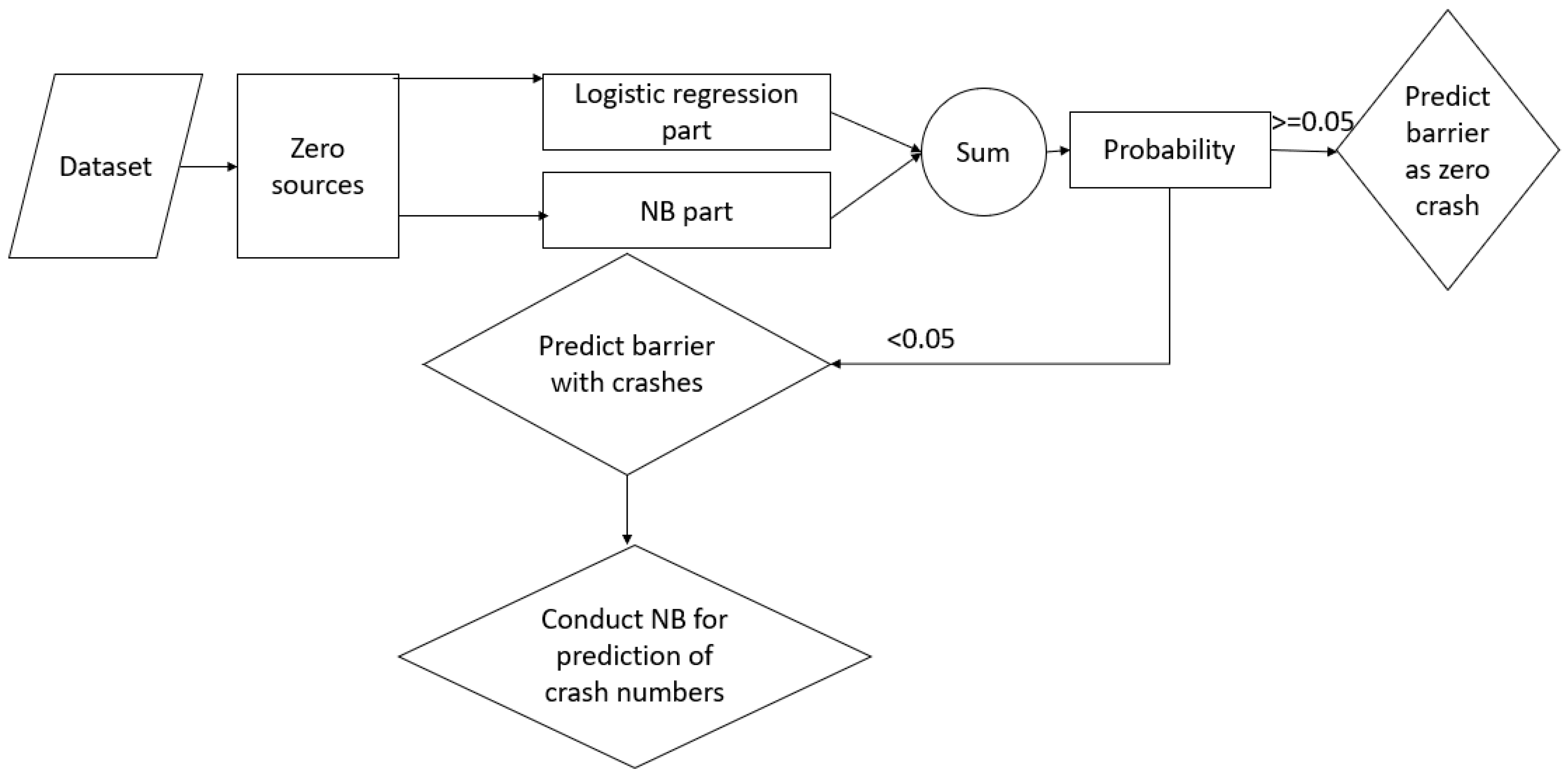
As discussed in the above section, the two-component models are very similar and the hurdle model could be considered as general form of ZI model. Thus, this study considered an application of ZI model only. The steps taken for optimization process, depicted in Figure 1, and could be outlined as follows:

• Conduct a two-component Bayesian hierarchical, along with a single-component model.
• After identifying a best fit model, e.g., two-component model, separate coefficients related to zero and count model, and convert them into equations.
• Calculate binary logistic regression, and zero count NB model, similar to Equation (1).

If the resultant value is greater than 0.5 stop and predict zero count barrier, otherwise

Use the second part of Equation (1) to calculate the count of barrier crash.

4.

If the probability of zero, $f_{zero}\left(0;z,\mathsf{\gamma }\right)$ is less than 0.5, calculate expected value of a negative binomial count model as follows:

$$\mathrm{count}-\mathrm{model}=\left(1-f_{zero}\left(0;z,\mathsf{\gamma }\right)\right)\times \exp (\alpha +{\beta }_1\times x_1+{\beta }_2\times x_2+\cdots +{\beta }_n\times x_n)$$

(6)

It should be noted that if a crash is predicted as having a predicted count of non-zero, this model can be used for predicting count of crashes. Furthermore, as can be seen from second part of Equation (1), the value of count needs to be multiplied by $1-f_{zero}\left(0;z,\mathsf{\gamma }\right)$. For our case, due to this value being very small, which will be explained later, this value is considered as 1 (1-0).

5. Model Syntax in JAGS

All the modeling is conducted in the context of Bayesian method. “Just another Gibbs sampler” (JAGS) package in R was used for the modeling process [13]. The Poisson model has been used as a starting point for analyzing any count modeling. Thus, a Poisson model was considered with a log link between conditional mean as $E\left(y_i|x_i\right]={\lambda }_i$, and linear predictor as ${\mu }_i={\displaystyle \sum }_j{\beta }_j{X}_{ij}$. In the syntax of the model, the two-part models should be defined explicitly: the first part distribution for the count model, and the second part as a logit model, Bernoulli distribution. Therefore, it is better to call this model a two-component model which could be applied as a hurdle or ZI model. For the ZI model, two distributions for the count part were considered: zero-inflated with negative binomial (ZINB), and Poisson (ZIP) distributions.

In the model syntax, the distributions for the second model component, count model, should be defined. Compared with Poisson distribution, negative binomial (NB) distribution required more parametrization to have an acceptable form, making it suitable for modeling sparse dataset. This would be implemented on observation i with success parameter of p_i and over-dispersion parameter of r, which is greater than 0. The success parameter can be written as follows:

$$p_i=\frac{r}{r+{\lambda }_i}$$

(7)

where ${\lambda }_i$, similar to Poisson, is a conditional mean which could be written as follows:

$$log{\lambda }_i={\displaystyle \sum }_j{\beta }_j{X}_{ij}$$

(8)

The above equation is similar to Equation (4), so no further explanation would be given.

It should be noted that a prior value of r should be set in the syntax of the model in JAGS. A uniform prior was set for this value with an upper bound of 50, and a lower bound of zero. In the syntax of JAGS, the negative binomial success could be written as follows:

$$p_i=\frac{r}{(r+1-zer{o}_{part})\times {\lambda }_i}$$

(9)

As can be seen from Equation (9), in general, if an observation does not belong to a zero part, the above equation would turn to the Equation (7) for Poisson distribution.

A hierarchical model could be written as follows:

$$\log \left(Y_{ij}\right)={\displaystyle \sum }_{j=1}^J{\displaystyle \sum }_{p=1}^P({\beta }_{0j}+{\beta }_p{X}_{ij})$$

(10)

where $Y_{ij}$ is a barrier crash EPDO for a certain barrier type, subscript i refers to an individual crash and subscript j refers to a hierarchies or levels, which is equal to the number of traffic barriers types as 3. For this study, p is the number of incorporated predictors in the count part. Here, as the random intercepts related to barrier type were considered only, the model coefficient would be similar across various barrier types, and only intercept would vary.

Due to the absence of prior information about the included predictors in the analysis, non-informative priors were set. It has been shown in the literature review that a choice of non-informative prior distribution for a variance parameter can impact the inferences significantly [14]. Thus, in this study, for the included predictors, a standard choice of the normal distribution with mean of 0, and a very high variance of 100,000 were considered. As in the syntax, precision needs to be set which is $\frac{1}{variance}$, this value is set in the Syntax. Furthermore, draws were obtained from 3 Markova Chain Monte Carlo (MCMC), with each chain consisting of 20,000 draw or iterations, in which 2500 of those draws were burned. Trace plot measures were used as measure for checking the mixing of the chains and estimates consistency across the chain.

The identification of a best fit model is important as the finalist model would be used for cost-benefit analysis. The deviance information criterion (DIC) was used as measure for model comparisons [15]. This is a generalization of the Akaike information criterion (AIC) in the Bayesian context. This method can be defined as a measure for complexity and goodness of fit, where complexity is linked to the number of included parameters, while the fit measure is related to deviance, and can be written as follows:

$$DIC=\overline{\mathit{D}(\varnothing )}+p\mathrm{D}$$

(11)

where, similar to AIC, $p\mathrm{D}$ is a number of included parameters. The model would be penalized for a higher number of incorporated parameters. $\overline{\mathit{D}\left(\mathit{\gamma }\right)}$ is deviance which could be written as the posterior mean of deviance as follows [16]:

$$\overline{\mathit{D}(\varnothing )}=E\left\{D(\varnothing )\right|\mathit{y}\}$$

(12)

where y is the dataset and $\varnothing$ are the unknown parameters. It should be noted that the above equation is not penalized by the model complexity. Furthermore, $\mathrm{D}(\varnothing )$, as an overall fit of a model (deviance), can be written as -2 times the log likelihood, as follows:

$$\mathit{D}(\varnothing )=-2logLik(\varnothing )|y)$$

(13)

A best fit model would be identified based on a lower value of DIC.

6. Cost-Benefit Analysis

For conducting any optimization process, the benefits and costs of any policy need to be carefully weighted. Welfare maximization has been highlighted as the objective of cost-benefit analysis [17].

The cost-benefit analysis relies on the Pareto-criterion for checking whether a project increases welfare or not. The idea states that the ideal welfare scenario would be achieved when an improved change makes some people better off while nobody would experience a loss. However, in practice, some projects make some people better off, while others would be worse off. Thus, the economists pledge to a less demanding state, stating that a project satisfies the criterion when those who benefit from a project compensate those who lose from it [17]. The same concept was implemented in this study: if, overall, the total benefit is positive, optimizing traffic barriers would be cost-effective, and a higher priority should be given to a higher benefit based on cost-benefit analysis. A period of 10 years was considered in this study for cost-benefit analysis, and the benefit could be written as follows:

$$\begin{array}{ll}Benefitover10& year\\ & ={\displaystyle {\displaystyle \sum }_{i=1}^{10}}(predictedcostwithnobarrierenhancemen{t}_i-(Resetcost\\ & +predictedFuturecos{t}_i)\end{array}$$

(14)

where i is a measurement for every year. In the above equation, costs would be estimated based on various years for various traffic count. Major costs, including reset or new barrier cost, would be executed in the first year. It should be noted that, for the incorporated barriers, box-beam and W-beam barriers heights can be reset, while for concrete barriers, the removal and rebuilding of concrete barriers would be needed to optimize heights.

Based on the last 10-year historical traffic data, the traffic on the state highway system was almost constant, while the traffic on interstate system increased by a rate of 4% in 10 years.

EPDO based on recommended WYDOT values for different crash types would be written as:

$$\begin{gathered} EPDOrate=Fatalcrashes+suspectedseriousinjury+suspectedminorinjury \\ +possibleinjury+Unknown+PDO \end{gathered}$$

(15)

The above equation after converting every crash severity level to PDO, in order, follows:

$$EPDOrate=277\times PDO+13\times PDO+4\times PDO+4\times PDO+4\times PDO+1\times PDO$$

(16)

In summary, the methodological steps taken in this study could be highlighted as follows:

• Identify all the barriers with crashes across highway and interstate systems in Wyoming.
• Identify the barrier which did not experience any crashes but are below/above recommended heights.
• Aggregate the crash data, data in steps 1 and 2, with traffic barrier dataset based on milepost, and roadway ID.
• Filter the data to include those barriers that are not based on standard heights, as “newdataset”.
• Identify the best distribution with a lowest DIC based on data in step 3.
• Convert the best fit model in step 5 into an equation.
• Implement a trained model in step 6 on dataset being based on current barrier geometric characteristics, and for each year an increase in traffic for interstate system only.
• Optimize the barriers to optimum height values based on the literature review, and conduct step 7 with the difference that an optimum value of barriers would be used.
• Based on step 8, convert EPDO into a cost and sum up the expected barriers crash cost for every year for barriers with optimum values and add the cost of height reset.
• Based on step 7, Convert the EPDO into a cost and sum up expected barriers crash cost for every year for barriers with no enhancement, and no cost of reset.
• Measure the difference between steps 9 and 10.
• Report the total of saving.
• Sort barriers based on highest benefits and report it.

7. Optimum Traffic Barrier Heights

The first step in the optimization process is to identify the optimum heights of barriers so the barriers would be set to that optimum value. Various values have been highlighted for both box beam and W-beam barriers ranging from 27 to 31 inches [2,18]. Based on the modeling results, a cutting point of 30 inches was chosen as a value that could optimize the benefit of the barriers. Furthermore, for concrete barriers, various values between 32 and 42 inches are proposed in the literature review [19,20,21]; a value of 40 inches was chosen to bring the concrete barriers to an optimum value.

It should be noted that the concrete barriers account for a total of 2% of all barriers, and the majority of these barriers in the dataset were higher than 42 inches. As a higher concrete barrier could not result in an underride crashes, those barriers were excluded from the optimization process, and only short concrete barriers were considered for optimization process.

8. Data

Three sources of datasets were aggregated for the final analysis. These data sources included: traffic, crashes, and barrier geometric characteristics. The crash and traffic datasets for this study originated from WYDOT. The crash data was filtered to incorporate crashes between 2007 and 2017. The traffic dataset included average annual daily traffic (AADT) and average annual truck traffic (ADTT). The response of the crash data was crash severity which was converted into EPDO based on the criteria highlighted by WYODOT (see Equation (16)).

The second dataset, barrier geometric, included various roadway and barrier geometric characteristics including: barriers types, lengths, offsets, heights, and various roadside geometric characteristics, such as shoulder width. This dataset also included the starting and ending mileposts of traffic barriers and roadway IDs. The crash data was separated into interstate and state highways systems. The data included only those crashes involving hitting a barrier as their first harmful event were included in the data set.

The crash dataset was aggregated across various barriers based on the milepost, direction of travel, and highway system. Due to low traffic on the state highway system, many traffic barriers have not been involved in crashes over the ten-year analysis period. As a result, a significant portion of these barriers on the state highway system are not within a recommended height. Thus, due to randomness of crashes and the fact that it is likely for these barriers to experience crashes, those barriers were added to the dataset resulting in a significant number of zero responses.

It should be noted that all the risky zero crash barriers and barriers that experienced at least a crash were used for training the model. Then, the trained model was implemented on those barriers that were not within the range of barrier designs. Thus, the information is presented in

Table 1. Summary statistics of important predictors: the whole data being used for training.

Variable ID	Variable Description	Mean	Variance	Min	Max
N = 2432			All barriers
	Box beam as reference, concrete as 2 and W-beam as 3	1.7	0.906	1	3
Response (EPDO)		7.6	1120.239	0	555
b1	AADT	2306	2,744,863.728	27	8853
b10	Restrain condition, having some form of restrain as reference (0), 1 otherwise	0.1	0.074	0	1
b12	Lighting conditions, light condition as reference (0), 1 otherwise	0.4	0.171	0	1
b2	Alcohol involvement, no alcohol involvement as reference (0), 1 otherwise	0.1	0.054	0	1
b3	Barrier height, continuous	29.6	9.652	<20	56
b4	Shoulder width, continuous	5.6	12.444	0	58
b5	Weather condition, clear weather condition as reference (0), 1 otherwise	0.5	0.179	0	1
b6	Roadway classification, state highway system as 0, 1 otherwise	0.5	0.248	0	1
b7	Gender, males as reference (0),1 otherwise	0.3	0.156	0	2
b8	Length, continuous	683	1.805	14	35,470
B17	Highway classification	0.4	0.248	0	1
b16	ADTT	483	208,279.501	2	2227

for the training data and

Table 2. Summary statistics of a data that a trained model is implemented on, under-design barriers.

N = 775			Risky Barriers
Response (EPDO)		3.9	580.963	0	308
	Box beam as reference, concrete as 2 and W-beam as 3	1.6	0.294	1	3
b1	AADT	199	26,905.84	3	972
b10	Restrain condition, having some form of restrain as reference (0), 1 otherwise	0.1	0.056	0	1
b12	Lighting conditions, light condition as reference (0), 1 otherwise	0.4	0.169	0	1
b2	Alcohol involvement, no alcohol involvement as reference (0), 1 otherwise	0.1	0.0601	0	1
b3	Barrier height, continuous	25	33.159	<20	57
b4	Shoulder width, continuous	4.9	12.923	0	19.4
b5	Weather condition, clear weather condition as reference (0), 1 otherwise	0.5	0.176	0	1
b6	Roadway classification, state highway system as 0, 1 otherwise	0.2	0.163	0	1
b7	Gender, males as reference (0),1 otherwise	0.3	0.151	0	1
b8	Length, continuous	571	1.251*E+06	2E+04	15
B17	Highway classification	0.205	0.163	0	1
b16	ADTT	415.47	169,643.7	2	1793

for the implementation of a trained model.

Both Table 1 and Table 2 included only those predictors that were found to be significant in the statistical analysis. Furthermore, variables IDs are presented as they were set in the syntax of the models in JAGS. It should be noted that although a categorical characteristic, binary, of barrier height and shoulder width were incorporated in the statistical analyses, the original characteristics of these two features were incorporated in Table 1 and Table 2 to provide a better idea of their characteristics for the readers.

According to Table 1 and Table 2, often a barrier may experience more than a single crash. For this scenario, the average of various drivers, weather, and road conditions were used as explanatory variables. For instance, if two drivers, one male driver as 0 and another female driver as 1, hit a barrier during the 10 year period, gender variable for that barrier ID would be set as the average of these two observations as 0.5. Furthermore, an average of the predictor highlights’ the distribution of that characteristics across specific barrier. For instance, roadway classification for Table 1 has a mean of 0.5, meaning that half of the barriers were located on state highway system while the other half were on the interstate system. This predictor changes to 0.2 in Table 2 as most of the under-design barriers are on the state highway system.

It should be noted that although the original values of AADT and length of barriers are presented in Table 1 and Table 2, these values were divided by 10 so those values would be comparable with other small binary predictors. Since the value of truck traffic is considerably smaller than the AADT value, the original value of this predictors is considered in the analysis. Again, a binary characteristics of shoulder width with a cutting point of 4.5 feet, and barrier height of 30 inches were used in the analyses.

9. Preprocessing Steps

Few points are worthy of being highlighted, regarding the preprocessing steps. First, as the response was EPDO, any variable, such as crash count or the severity of crashes, was removed from the variables, due to the irrelevance and high multicollinearity. Noisy variables, such as crash/barriers IDs, were removed from the data before conducting any analysis. Various range or values of shoulder width and barrier heights were considered and evaluated to come up with the range that significantly impact the EPDO crashes. This is due to the importance of those predictors for optimization process. All the important predictors were incorporated in the analysis and removed one by one based on the worst confidence interval. Although drivers’ factors were set constant in the machine learning process, those were incorporated in the model to enhance the model performance.

10. Results

The descriptions of the analysis are presented in three subsections. The first subsection summarizes the best fit prediction model. The second subsection details the mathematical process of the best identified two-component model in predicting EPDO crashes. The last subsection summarizes the optimization results. As in the syntax of JAGS, two models, binary logistic, and the count model should be defined; both the ZI and hurdle model could be inferred from the results with some modifications.

11. Best Fit Model

Three models were compared to select the best model for conducting the optimization process. Since Poisson distribution was used as a starting technique for modeling the count response, Bayesian hierarchical two-component model with the Poisson distribution was considered in addition to NB distribution. Besides those two models, a one-layer NB Bayesian hierarchical technique was considered. Similar predictors were considered for the three models so that a fair comparison could be made. Truck traffic, instead of AADT, was used for the first layer, logistic regression, of the two-component models as it was found that ADTT to be significant for the logistic regression part.

Since the one-layer NB could accommodate all the predictors in one layer and there was a correlation between ADTT and AADT, ADTT was not considered in that model. However, as discussed in the method section, DIC could penalize for the number of included predictors. The results are presented in

Table 3. Estimation results of two-layer model, with Poisson distribution for the second layer.

	Mean	SD	2.50%	97.50%
2nd layer, Poisson model
alpha1	1.739	0.025	1.69	1.788
alpha2	2.521	0.038	2.447	2.595
alpha3	2.346	0.022	2.302	2.39
b1	0.001	0.0002	0.001	0.001
b10	1.351	0.025	1.301	1.4
b12	−0.361	0.021	−0.404	−0.32
b2	0.917	0.034	0.849	0.981
b3	−0.066	0.021	−0.107	−0.026
b4	−0.334	0.022	−0.377	−0.291
b5	−0.667	0.02	−0.707	−0.627
b6	0.299	0.022	0.258	0.343
b7	−0.335	0.023	−0.379	−0.29
b8	0.001	0.0001	0.001	0.001
b9	0.331	0.036	0.26	0.399
1st layer, logistic regression
alpha	−0.88	0.074	−1.027	−0.734
b17	−3.034	0.19	−3.415	−2.668
B16	0.001	0	0.001	0.002
DIC = 54,658.1

,

Table 4. Estimation results of single-layer model, with NB distribution.

	Mean	SD	2.50%	97.50%
alpha1	0.278	0.087	0.108	0.45
alpha2	0.429	0.153	0.148	0.756
alpha3	0.446	0.085	0.28	0.613
b1	0.001	0.0002	0.0009	0.01
b10	2.213	0.156	1.909	2.537
b12	0.403	0.098	0.216	0.6
b2	1.991	0.19	1.614	2.373
b3	0.199	0.087	0.028	0.369
b4	0.138	0.084	−0.028	0.302
b5	−0.328	0.086	−0.497	−0.16
b6	0.703	0.086	0.537	0.875
b7	0.438	0.102	0.241	0.642
b8	0.005	0.0001	0.004	0.006
b9	−0.42	0.15	−0.716	−0.12
DIC = 12,679.8

and

Table 5. Estimation results of two-layer model, with NB distribution for the second layer.

	Mean	SD	2.50%	97.50%
2nd layer, NB model
alpha1	0.472	0.09	0.295	0.65
alpha2	0.564	0.142	0.307	0.876
alpha3	0.564	0.088	0.394	0.734
b1	0.001	0.0009	0.001	0.002
b10	2.134	0.152	1.837	2.436
b12	0.252	0.097	0.06	0.441
b2	1.867	0.189	1.501	2.24
b3	0.189	0.088	0.018	0.363
b4	0.087	0.083	−0.073	0.249
b5	−0.441	0.086	−0.609	−0.27
b6	0.501	0.083	0.344	0.667
b7	0.362	0.101	0.165	0.56
b8	0.005	0.001	0.004	0.005
b9	−0.351	0.151	−0.645	−0.057
1st layer, logistic regression
alpha	−13.593	2.197	−17.518	−9.327
b17	−35.049	8.392	−47.179	−19.414
b16	0.02	0.004	0.013	0.027
DIC = 12,558.7

.

Although the signs/directions are consistent across one layer and two-layer models with NB distribution, important variations could be observed between those models and two-layer Poisson distribution. The differences are especially important across b12 (Lighting conditions), b7 (gender), and b9 (interaction term). This is expected as Poisson cannot accommodate over-dispersion and an excess number of zeroes. This model also resulted in a worst fit (DIC = 54,685) compared with two-layer NB (DIC = 12,559) and one-layer NB (DIC = 12,680).

Based on the discussed DIC values, the two-layer NB provides the best fit model. The results indicated that alcohol involvement, clear weather conditions, being a female driver, and having an improper restrain increased the EPDO of barrier crashes. On the other hand, driving in light conditions decreased the EPDO crashes. It should be noted that the AADT and length of barriers were incorporated in the analysis to account for an exposure effect. As expected, for the higher barrier length and AADT, higher EPDO barrier crashes were observed. As discussed in the method section, these variables were divided by 10 before implementation.

For the first layer of the models, two variables were incorporated: highway system and truck traffic. Results indicated that having a barrier on the interstate system decreased the odds of experiencing any crash compared with highway system. Although this result seems counterintuitive, the difference between experiencing a crash and experiencing a higher EPDO crash should be noted. Truck traffic similar to the second layer for the exposure effect was considered. Similarly, higher ADTT moves barriers from a no crash area to a crash area.

In terms of interception, it should be noted that alpha 1 is for box beam, alpha 2 is for concrete, and the third alpha is related to W-beam. As can be seen from the magnitudes of these three intercepts, box beam has a lower EPDO crash compared with the other two barriers.

Comparing Table 3 and Table 5 in terms of confidence interval (CI) and SD, a few observations can be made. Standard errors of Naïve estimates, Poisson, are smaller than NB. In addition, probabilities coverage of CI are lower compared with NB. This would result in erroneous inference due to ignoring over-dispersion, which is evidence from point estimates in terms of magnitude and signs.

12. Mathematical Optimization Process

After identifying the two-layer model as a best fit model, the results of this analysis would be converted into an equation which can be used in the optimization process. Due to similarities of both ZI and hurdle model, and as ZI could be considered as general form of hurdle model, this section will mainly focus on ZI model. At the end of the section, a contrast between these two models would be made. As discussed in the syntax of JAGS, two components, count and logistics, need to be clarified so for machine learning both hurdle and ZI models with some modifications could be considered.

Zeros in ZI model would be produced with 2 processes. A zero through Bernoulli/binary logistic and through NB distributions. For this two-component model, first it should be clarified whether a barrier has experienced a crash or not. To fulfill this objective, the odds of zero crash, success, is equal to the exponential of the included predictors for this layer. This resulted in a maximum value/probability of 0.02 indicating that no crash would be predicted with this process. Up to this point, Hurdle and ZI are similar: no zero-barrier crash. However, there is an extra process of creating zero for ZI model.

The second zero-producing process is related to the count component, NB model, being shown in Equation (2). Over-dispersion parameter was calculated for NB model as 0.66. After implementing the formula based on Equation (2), a maximum probability of zero was obtained as 0.452. After adding up this zero-producing process with logistic regression, it resulted in a maximum probability of zero barrier as 0.453. This indicates that none of the zero process in ZI model could predict zero. Thus, ZI and hurdle are similar up to this point.

Moving to the second layer for predicting barrier crash count. The difference between the two-layer models is just $1-f_{count}\left(0;x,\mathsf{\beta }\right)$ in the denominator of the hurdle model in Equation (5). $f_{count}\left(0;x,\mathsf{\beta }\right)$ is ranging from a minimum value of 0.0006 to a maximum value of 0.452. Thus, the denominator of Equation (5) result in a value less than 1, which increase the predicted count of hurdle model compared with ZI model. However, as discussed, the results of the next section are presented based on ZI model.

In summary, although the two layers of model was used for accommodating extra zeroes, machine learning technique was not able to predict any zero-crash barrier. This is likely due to randomness of crashes and especially barrier crashes. Thus, just based on traffic and highway system the model is not able to predict if a barrier has experienced any crashes or not.

13. Optimization Results

This section would highlight the results of ZINB machine learning technique in identification of benefit associated with various barriers.

Table 6. The top critical highway-system barriers, sorted based on highest benefits.

Interstate/Highway	Highway Classification	Barrier ID	Shoulder Width	Current EPDO	Barrier Height	Type of Barrier	Length of Barrier (ft)	AADT	Overall Benefit in 10 Years	Rank
ML2000B	State Highway	4115	5	13	26	Box-beam	241	4810	1,377,961	1
ML90I	Interstate	4319	11	4	26	Box-beam	470	1983	378,591	2
ML80I	Interstate	5079	7	1	26	concrete	63	3617	373,292	3
ML80D	Interstate	6545	7	17	26	Box-beam	241	5128	277,206	4
ML25D	Interstate	6862	10	4	23	W-beam	1514	3815	261,031	5
ML34B	State Highway	4058	8	4	24	Box-beam	152	2517	184,740	6
ML10B	State Highway	3751	6	4	25	W-beam	1064	3670	145,149	7
ML35B	State Highway	2077	7	5	26	W-beam	352	226	124,971	8
ML4200B	State Highway	607	7	9	26	Box-beam	750	6719	114,334	9
ML20B	State Highway	3054	17	4	25	concrete	165	719	110,451	10
ML10B	State Highway	3728	7	1	26	W-beam	1227	3670	105,874	11
ML25I	Interstate	6098	5	21	25	Box-beam	827	2943	83,728	12
ML25I	Interstate	6884	10	18	26	W-beam	476	3653	81,578	13
ML80I	Interstate	6475	6	11	26	Box-beam	269	5138	69,693	14
ML80I	Interstate	6386	7	2	23	Box-beam	291	3617	67,923	15
ML80D	Interstate	4960	5	0	<22	Box-beam	96	5878	51,798	16
ML10B	State Highway	3654	6	2	25	W-beam	465	3670	51,746	17
ML80D	Interstate	6524	10	287	26	Box-beam	208	5128	48,250	18
ML90I	Interstate	7550	7	6	24	Box-beam	858	1812	48,045	19
ML80D	Interstate	5030	5	0	25	Box-beam	168	5138	46,531	20
ML80I	Interstate	6395	5	0	25	W-beam	52	3617	45,940	21
ML80D	Interstate	6379	5	0	25	W-beam	151	3902	45,319	22
ML25I	Interstate	6894	5	0	22	W-beam	127	3653	44,608	23
ML25D	Interstate	6872	5	0	20	W-beam	216	3815	43,602	24
ML25D	Interstate	5831	5	0	25	W-beam	216	3815	43,600	25
Total		-	-	-	-		84 miles	-	$3,314,766

highlight the highest benefits associated with the included barriers. The main purpose of using both interstate and state highway in the model was to provide one optimized list for all roads maintained by WYDOT in the state.

As the main analysis was conducted on EPDO, those crashes were converted to monetary measure so the cost of enhancement could be incorporated as shown in Equation (16). The advantages of incorporating AADT and barrier lengths could be observed in Table 6 where the highest benefits are not necessarily related to barriers with highest length or highest traffic. However, it was found the majority of barriers with highest associated benefits are related on the interstate system which includes I-80, I-25 and I-90. In summary, it was found that by investing about 10 million dollars in barriers enhancement, WYDOT would not expect just to recover the spent money but also make more than 3 million dollars in crash saving. It should be noted that 775 barrier IDs in both state highway and interstate were optimized due to being below standard. Table 6 only present the topmost beneficent barriers to be optimized. The sum at the bottom of Table 5 also presents the total of benefit considering the associated costs of all barriers enhancement.

At the end, it is worth comparing the performance of the predicted values and real values of EPDO. The values are presented in

Table 7. Some statistics about predicted and real EPDO based on ZI method.

	Variance	Min	Max
Predicted EPDO	90	1	198
Real EPDO	168	0	287
Root mean square error = 35,064

. Few points can be made from Table 7. First, the variance of predicted EPDO is smaller than the real EPDO. This is expected as the algorithm follows some predefined rules so the difference across various values follow certain rule without a huge difference resulting in a lower variance. On the other hand, the real EPDO has a higher value, which could be linked to the randomness of crashes due to differences across drivers. Another point worthy to mention is minimum values. While the minimum value of EPDO is zero, the machine learning technique could not identify any barriers as safe. This has been discussed in the literature review extensively that crashes are random and no location/barrier is inherently safe.

14. Conclusions

This study was conducted with an objective of implementing a cost-benefit analysis of traffic barrier geometric enhancement. The traffic barriers in the state is characterized by a preponderance of zeros due to low traffic volumes. Most of these zero-crash barriers have not received any crashes due to the nature of crash randomness and low traffic volumes. A significant portion of those barriers need an immediate attention since they are not within recommended geometric characteristics. Thus, this project was initiated by WYDOT to find a methodological approach to provide a monetary benefit of optimizing those barriers. In addition, due to limited budget of WYDOT, those barriers need to be prioritized so barriers with higher benefit could be optimized first.

The main step in conducting an optimization technique is to identify a best fit model that can model sparse EPDO barrier crashes with presence of excess zeroes. To achieve this objective, various two-component models with various count distributions, in addition to a simple count model, were considered. In order to account for the unobserved heterogeneity across various crash observations due to traffic barrier types, the association was introduced through suitable random effects hierarchical model. All the analyses were conducted in the Bayesian framework. The two-component distribution is a mixture of two distribution, Bernoulli and NB or Poisson, while a single-component model was Bayesian hierarchical NB model.

Deviance information criterion (DIC) was used for model selection. A two-component model with NB as a count part was identified to perform best compared with all other considered models. A comprehensive discussion was made about various scenarios of two popular two-component models, zero inflated and hurdle model. These two models were found to be very similar in prediction of barrier EPDOs, especially in predicting zeroes. The zero-parts of these models include traffic and highway classification type. The first layers of both models could not predict any zero-crash barriers. In other words, no barriers could be predicted by models as safe, even if the current traffic condition persist. This could be justified by the main reason of the randomness of crashes. A barrier at a very low traffic could still be hit by erroneous activities resulted from a careless driver. This is why a model identified a significant portion of most hazardous barriers among those barriers that have not experiences any crash, EPDO=0, as shown in Table 6. Despite having a lower percentage of interstate barriers in the dataset, based on optimization results, most of the identified barriers to be enhanced first belong to the interstate system.

The results also indicated that after investing the money into upgrading barriers, WYDOT is not only expected to regain the investment over ten years, but also to gain more than 3 million dollars in crash savings. The results of the implemented cost-benefit analysis presented in this paper do not just provide WYDOT with the expected benefits from upgraded barriers, but it also prioritizes barriers based on higher benefits so that WYDOT can allocate available funding to enhance barriers annually based on available budgets. The process described in this paper can be utilized by other DOTS to optimize the expenditures on updating the road barriers in their states.