Article

The Model Order Reduction Method as an Effective Way to Implement GPC Controller for Multidimensional Objects

by
Sebastian Plamowski
1,* and
Richard W Kephart
2
1
Institute of Control and Computation Engineering, Warsaw University of Technology, Plac Politechniki 1, 00-661 Warszawa, Poland
2
Emerson Process Management, 200 Beta Dr, Pittsburgh, PA 15238, USA
*
Author to whom correspondence should be addressed.
Algorithms 2020, 13(8), 178; https://doi.org/10.3390/a13080178
Submission received: 2 June 2020 / Revised: 17 July 2020 / Accepted: 20 July 2020 / Published: 23 July 2020
(This article belongs to the Special Issue Model Predictive Control: Algorithms and Applications)

Abstract

:
The paper addresses issues associated with implementing GPC controllers in systems with multiple input signals. Depending on the method of identification, the resulting models may be of a high order and when applied to a control/regulation law, may result in numerical errors due to the limitations of representing values in double-precision floating point numbers. This phenomenon is to be avoided, because even if the model is correct, the resulting numerical errors will lead to poor control performance. An effective way to identify, and at the same time eliminate, this unfavorable feature is to reduce the model order. A method of model order reduction is presented in this paper that effectively mitigates these issues. In this paper, the Generalized Predictive Control (GPC) algorithm is presented, followed by a discussion of the conditions that result in high order models. Examples are included where the discussed problem is demonstrated along with the subsequent results after the reduction. The obtained results and formulated conclusions are valuable for industry practitioners who implement a predictive control in industry.

1. Introduction

Model Predictive Control (MPC) algorithms [1,2,3,4,5,6] are frequently used in industrial applications [7], especially as a technique for efficient control of Multiple-Input Multiple-Output (MIMO) processes. Compared with the classical PID controller, MPC algorithms give very good control quality and tuning is much easier, especially for non-minimum phase objects, objects with long time delays, as well as MIMO objects with internal coupling between inputs and outputs. Furthermore, in MPC, unlike PID control, all necessary constraints may be incorporated systematically in the control law. Additionally, MPC can be applied to nonlinear systems [8,9,10] using the structure of fuzzy models [11,12,13,14,15,16,17] or online linearization of the process model at each MPC algorithm iteration [18,19]. In large-scale industrial applications, MPC algorithms are implemented in Distributed Control Systems (DCS) using Programmable Logic Controllers (PLC) [20] or specialized industrial controllers [21]. Whereas in embedded systems, microcontrollers [22] or Field Programmable Gate Arrays (FPGA) [23] are typically used as hardware platforms.
Recent years have seen an increase in the development of predictive control techniques [24,25,26] used in both the lower levels, which have typically been thought of as base control, as well as the upper-level supervisory control layer, which may also include the optimization functions. It is worth noting that the explosive increase in computing power and capabilities of embedded controllers is causing the boundaries of the traditional layered control structure [27] to become blurred as the specific functions performed at each layer become less distinct.
This is one of the main reasons for the popularization of multidimensional predictive control techniques.
Despite these points, the use of advanced predictive control techniques can be difficult in some cases. There is extensive literature related to the limitations, advantages, and disadvantages of the use of advanced control systems. The authors draw attention to modeling problems and issues of inaccuracy of internal models used in predictive controllers [28,29]. The issue of calculations and memory requirements needed to run predictive controllers was also discussed [21]. In addition to general problems, there are problems that appear only for certain types of predictive control algorithms.
This work discusses the implementation of the General Predictive Control (GPC) algorithm for a multi-input process. The GPC algorithm originated in the late 1980s [30,31,32,33] and historically it is included in the second-generation algorithms [26]. The algorithm uses an internal model in the form of a discrete transfer function that defines the dynamic input-output relationships between the model inputs and outputs. The model inputs are the control system Manipulated Variable (MV) outputs as well as the Disturbance Variables (DV). The model outputs are the Controlled Variables (CV), which are the inputs to the control system. Due to the relatively simple yet universal form of the internal model, this algorithm has become very popular and particularly in the academic community. It is worth mentioning that the first theoretical studies proving stability were derived for algorithms derived from the GPC algorithm. The most important ones are CRHPC (Constrained Receding Horizon Predictive Control) [34] and SIORHC (Stabilizing Input Output Receding Horizon Control) [35], which were based on the concept of additional equalization constraints of the output signal.
The GPC algorithm uses a transfer function model to predict future CV values. Unfortunately, in some cases, particularly when the process has many inputs, the resulting internal model may be of high order. This can lead to numerical errors and ultimately to instability of the algorithm. The aim of this article is to show this undesirable property, which was noticed during the design phase of a GPC algorithm in a DCS system and persisted during the implementation phase at the sites. This property is visible only in certain conditions, which unfortunately quite often occur during implementation of advanced automation solutions in the real objects and are not referred in the literature. Additionally, this situation can be difficult to recognize since the effects are gradual in nature. Numerical problems appear gradually with increasing model order and occur during the internal model prediction stage of which the results are not directly visible outside of the algorithm. This subject is approached from the perspective of an actual control system project and utilizes the context of the GPC algorithm to illustrate the point. The solution presented is intended to be a practical solution. However, the problem does provide motivation for additional work in the area of prediction algorithms and their methods of implementation.
In the following sections of the paper, we will explore the conditions that result in high order models as well as present specific examples to illustrate the problem. Several methods that can be used to reduce the model order are discussed. A practical approximation method that is based on engineering judgement is presented, which that avoids resulting high order models. The presented method of order reduction is one of the possible approaches. This approach was chosen to be easy to apply by process engineers. There are many other reduction methods listed in this article but not investigated in detail since the aim of this article is not to compare the quality of the applied model reduction methods but to show the dangerous properties of the GPC algorithm and to justify the necessity of taking certain actions. The model order reduction method has its limitations and does not exhaust all possibilities of solving the problem. Alternative approaches are listed in the summary.
All results presented in this paper comes from simulations performed in MATLAB.

2. GPC Problem Formulation

2.1. Predictive Controller Formulation

Let n u and n y denote the number of process inputs (manipulated variables) and outputs (controlled variables), respectively, i.e., u = [ u 1 u n u ] T , y = [ y 1 y n y ] T . In the more general formulation of MPC, the vector of decision variables calculated at each sampling instant, k = 0 , 1 , 2 , , has the length of n u N u and consists of the current and future increments of the manipulated variables
Δ u ( k ) = [ Δ u ( k | k ) Δ u ( k + N u 1 | k ) ]
where Δ u ( k + p | k ) denotes increments of the manipulated variables for the future sampling instant k + p calculated at the current instant k , N u is the control horizon. The rudimentary MPC optimization problem is:
min Δ u ( k ) { p = 1 N y sp ( k + p | k ) y ^ ( k + p | k ) Ψ p 2 + p = 1 N u 1 Δ u ( k + p | k ) Λ p 2 }
subject to
u min u ( k + p | k ) u max ,   p = 0 , , N u 1
Δ u max u ( k + p | k ) Δ u max ,   p = 0 , , N u 1
The symbols y sp ( k + p | k ) and y ^ ( k + p | k ) denote the set-point trajectory and the predicted trajectory for the sampling instant k + p calculated at the instant k , the prediction horizon is N . The weighting matrices Ψ p = diag ( ψ p , 1 , , ψ p , n y ) and Λ p = diag ( λ p , 1 , , λ p , n u ) are of dimensionality n y × n y and n u × n u , respectively. The minimal and maximal values of the manipulated variables are denoted by u min and u max , respectively; the maximal rate of change of the manipulated variables is Δ u max . At each sampling instant, having calculated n u N u future increments of the manipulated variables over the control horizon (1), only the increments for the current time step are applied to the process.
The basic optimization problem (2) is the same in all MPC algorithms, even though the implementation details differ due to the fact that different types of dynamical models utilize different prediction equations [1,2,36]. When the linear model is used for prediction, a Quadratic Programming (QP) optimization problem results from the control law formulation, which may be solved by readily available solvers. Although the QP solver results in a more mathematically tractable problem, it does impose increased requirements on memory resources and CPU capacity. In typical industrial applications, MPC with on-line quadratic optimization is only practical for rather moderate numbers of process inputs and outputs [3]. Furthermore, the prediction horizon and particularly the control horizon have a significant impact on the resulting computational complexity and execution time necessary to complete the calculations at each sampling instant, which imposes limits on the control system’s ability to implement the optimization problem in real-time.

2.2. Construction of GPC Algorithm

In the GPC algorithm, the dynamics of the control object are modeled in the form of a discrete transfer function. In order to simplify the explanation, the model in the structure of Multiple Input Single Output (MISO) is presented in (3):
y ^ k = A T Y k 1 + B Δ U k M V _ P + D Δ U k D V _ P
A is a vector of model coefficients associated with historical values of the output given by (4):
A = [ a 1 a m a x _ n ]
where m a x _ n defines the number of the coefficients and order of the model denominator. Y k 1 is a vector of the past values of model outputs given by (5):
Y k 1 = [ y k 1 y k m a x _ n ]
B is a vector of model coefficients associated with historical values of the inputs (MVs signals) given by (6):
B = [ B ( 0 ) B ( m a x _ m ) ] = [ [ b 0 ( 1 ) b 0 ( n M V ) ] [ b m a x _ m ( 1 ) b m a x _ m ( n M V ) ] ]
m a x _ m defines the maximum number of coefficients for the MV inputs (model order), n M V defines number of MVs inputs. Vector of the past values of MVs is given by (7), where m v 1 to n M V define index of MV inputs, d e l a y m v 1 to d e l a y n M V defines delay values for each MV inputs.
Δ U k M V _ P = [ [ Δ u k d e l a y m v 1 ( m v 1 ) Δ u k d e l a y n M V ( n M V ) ] [ Δ u k m a x _ m d e l a y m v 1 ( m v 1 ) Δ u k m a x _ m d e l a y n M V ( n M V ) ] ]
D is a vector of model coefficients associated with the historical value of the Disturbance Variable inputs (DV signals) given by (8):
D = [ D ( 0 ) D ( m a x _ l ) ] = [ [ d 0 ( 1 ) d 0 ( n D V ) ] [ d m a x _ l ( 1 ) d m a x _ l ( n D V ) ] ]
m a x _ l defines the maximum number of coefficients for the DV inputs (model order), n D V defines number of DV inputs. The vector of the past values of DVs is given by (9), where d v 1 to n D V define the index of DV inputs, d e l a y d v 1 to d e l a y n D V defines delay values for each of the DV inputs.
Δ U k D V _ P = [ [ Δ u k d e l a y d v 1 ( d v 1 ) Δ u k d e l a y n D V ( n D V ) ] [ Δ u k m a x _ l d e l a y d v 1 ( d v 1 ) Δ u k m a x _ l d e l a y n D V ( n D V ) ] ]
In each timestep, the GPC algorithm solves the optimization problem defined by (2). The algorithm calculates the optimal trajectory of the CVs, which minimizes the difference between setpoint and predicted model outputs while minimizing the changes of MVs signals. The predicted model outputs are calculated using general model formula (3) based on past outputs of MVs and DVs values and predicted (i.e., calculated by GPC algorithm) MVs. The accuracy of the model predictions is critical to the correct operation of the GPC algorithm.

3. Process Identification

GPC control algorithm is based on a discrete time model. Although this type of model can be obtained directly from mathematical or physics equations, in actual practice, it is more common to obtain the discrete time model empirically using a system identification process. The complexity of industrial processes typically requires that the model be constrained to be a maximum of 3rd order to accurately capture the relationship between input and output. The generic form of model is shown in (10):
Y ( s ) U ( s ) = G a i n ( R 1 s + Q 1 ) ( R 2 s + Q 2 ) ( T 1 s + 1 ) ( T 1 s + 1 ) ( T 1 s + 1 ) e s t
where Q 1 and Q 2 can be equal 1 , 0 or 1 . The parameters R 1 , R 2 , T 1 , T 2 , and T 3 and process delay in the real project are identified experimentally, where the experiment depends on the specific industrial installation and used equipment.
Two approaches are used to identify models. The first one assumes that it is possible to stimulate all input signals simultaneously in such a way that the contribution of each individual term of the transfer function can be isolated. This is not always possible and is particularly difficult during closed loop operation.
The second method is based on the identification of SISO models. In this method, the relationships between all inputs and outputs are identified independently using bump-test experiments on the actual plant and typically without closed loop control—usually by placing the associated control loops in manual. The bump-test is accomplished by applying an excitation signal to each input, u (n), where the excitation signal is a step input. In actual practice, a true step may not be realizable, but a signal that closely approximates a step typically provides acceptable results. The model structure for one output is shown in Figure 1.
The identification of individual models is more effort-intensive but is straightforward and intuitive to understand, and it eliminates the problem of the influences of individual inputs on each other. This type of modeling is widely used in industry for model-based control. The model presented in Figure 1 cannot be applied directly to the GPC algorithm as the transfer function model must be reduced to a common denominator to match the general form shown in (3).
If every transfer function of the SISO model can be described as a quotient, the nominator N and the denominator D as showed below (11):
T x ( s ) = N x ( s ) D x ( s )
the sum of e.g., 3 models reduced to the common denominator is shown in (12).
T ( s ) = N 1 ( s ) D 2 ( s ) D 3 ( s ) D 1 ( s ) D 2 ( s ) D 3 ( s ) + N 2 ( s ) D 1 ( s ) D 3 ( s ) D 1 ( s ) D 2 ( s ) D 3 ( s ) + N 3 ( s ) D 1 ( s ) D 2 ( s ) D 1 ( s ) D 2 ( s ) D 3 ( s )
This process of reducing the models to a common denominator is critical because it can lead to high-order models and consequently to numerical issues in the actual implementation in software.

4. Example Models

4.1. Two Input-Two Output Model

This example utilizes a model with two inputs and two outputs. Both outputs depend on inputs in the same way, i.e., the model consists of two identical MISO models. The relationship between each input and output is described by independent transfer functions given by (13) and (14):
T 1 ( s ) = Y ( s ) U 1 ( s ) = 1 ( 120 s 1 ) ( 280 s + 1 ) ( 100 s + 1 ) ( 150 s + 1 ) ( 200 s + 1 )
T 2 ( s ) = Y ( s ) U 2 ( s ) = 1 ( 20 s 1 ) ( 40 s + 1 ) ( 50 s + 1 ) ( 70 s + 1 ) ( 180 s + 1 )
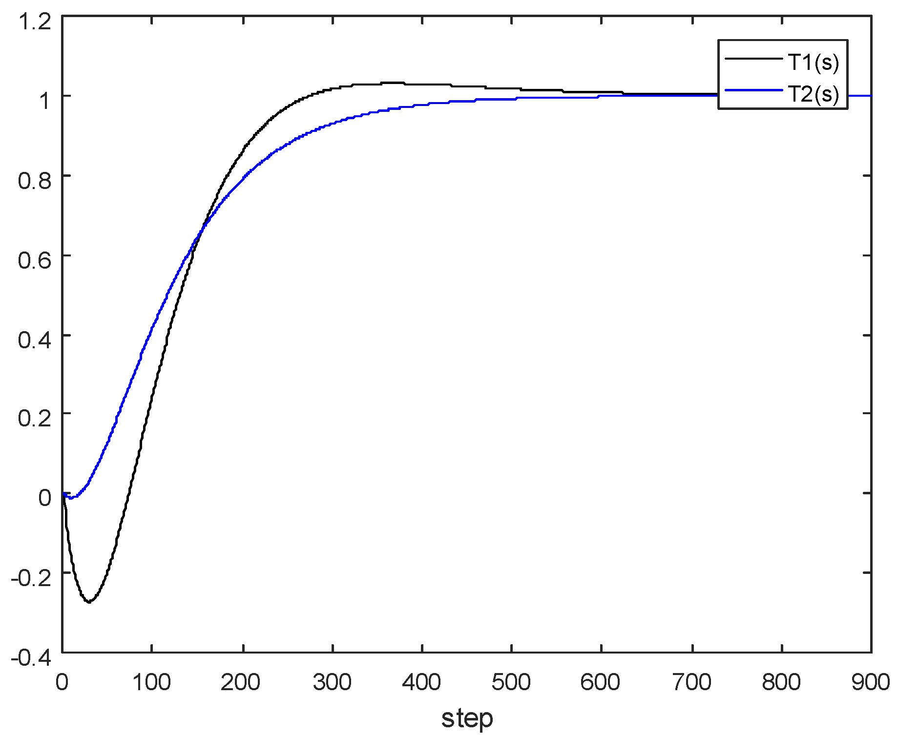
The transfer functions used in the examples structurally correspond to the third order models used in the DCS software to identify industrial process models given by (10). The values of time constants used in the examples were invented to show the problem of creating high-order models. Each sub-model was discretized with sample times of 2s and simulated as a step response for an 1800 s time-horizon, which is 900 time-steps, shown in Figure 2.

4.2. Transformation to GPC Internal Model Format

In the next step, the models are reduced to a common denominator and added as shown in (15) in order to meet requirements for the GPC internal model form shown in (3):
T ( s ) = T 1 ( s ) + T 2 ( s )
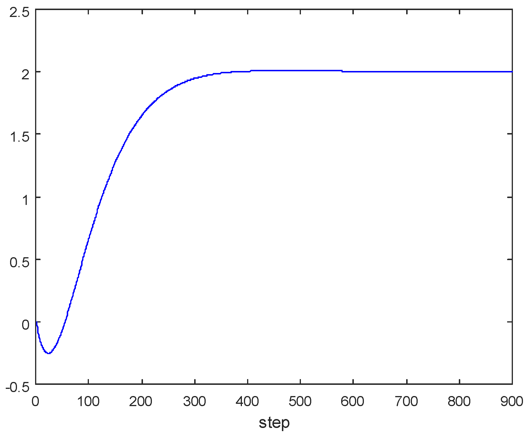
As a result, a 6th order model was obtained; a step response of the model is shown below in Figure 3.
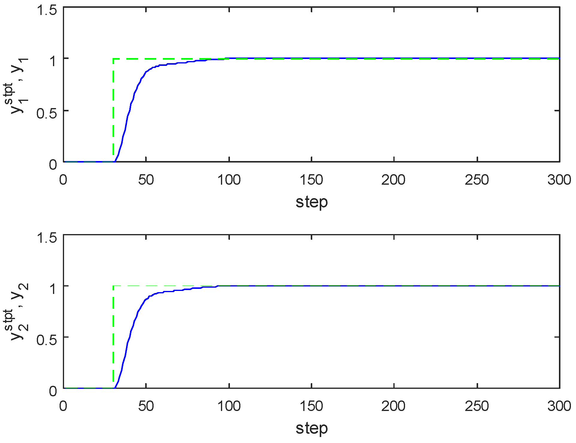
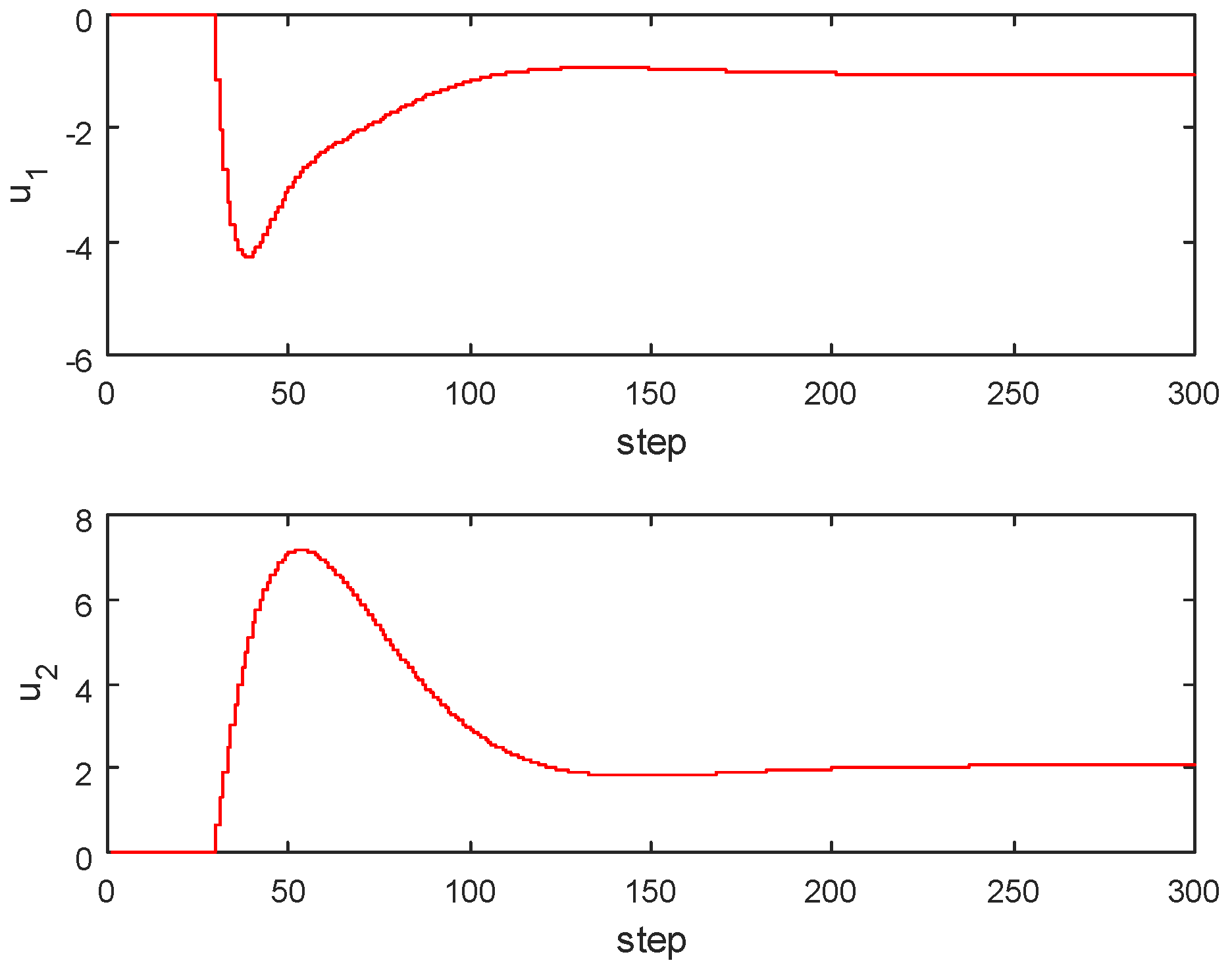
GPC controller with a 6th order internal model was simulated in the closed loop; the following values of tuning parameters were used: control horizon N u = 20 , prediction horizon N = 400 , and matrix R as a unit matrix. The original model shown in (12), which was before the reduction to a common denominator, was used as the plant in the simulation, where each input-output relationship is simulated independently using (15). The closed loop operation is stable, and the GPC algorithm works correctly. The results are shown in Figure 4 and Figure 5.
The same experiment was repeated for a model the included an additional input. The results are discussed in the next section.

4.3. Three Input-Three Output Model

The model presented in Section 4.1 was extended about one more input, as described by transfer function T 3 ( s ) (16):
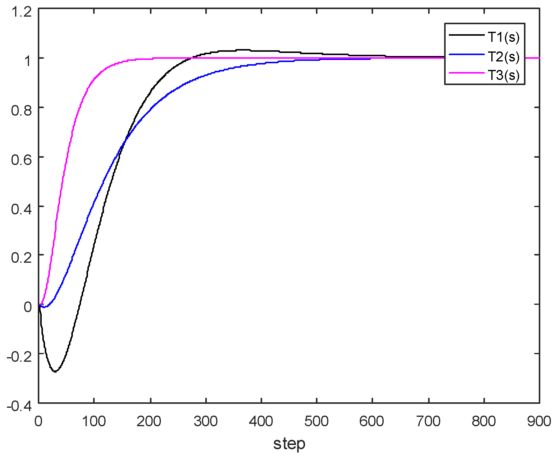
T 3 ( s ) = Y ( s ) U 3 ( s ) = 1 ( 10 s + 1 ) ( 30 s + 1 ) ( 60 s + 1 )
As in the two input-two output case, each sub-model was discretized with a sample time of 2 s. and the step response was simulated over an 1800 s time horizon, which again is 900 time-steps. The resulting step response from each input is presented in Figure 6.
As in the previous example, the models were reduced to a common denominator and added as shown in (17) in order to meet the requirements for the GPC internal model form shown in (3).
T ( s ) = T 1 ( s ) + T 2 ( s ) + T 3 ( s )
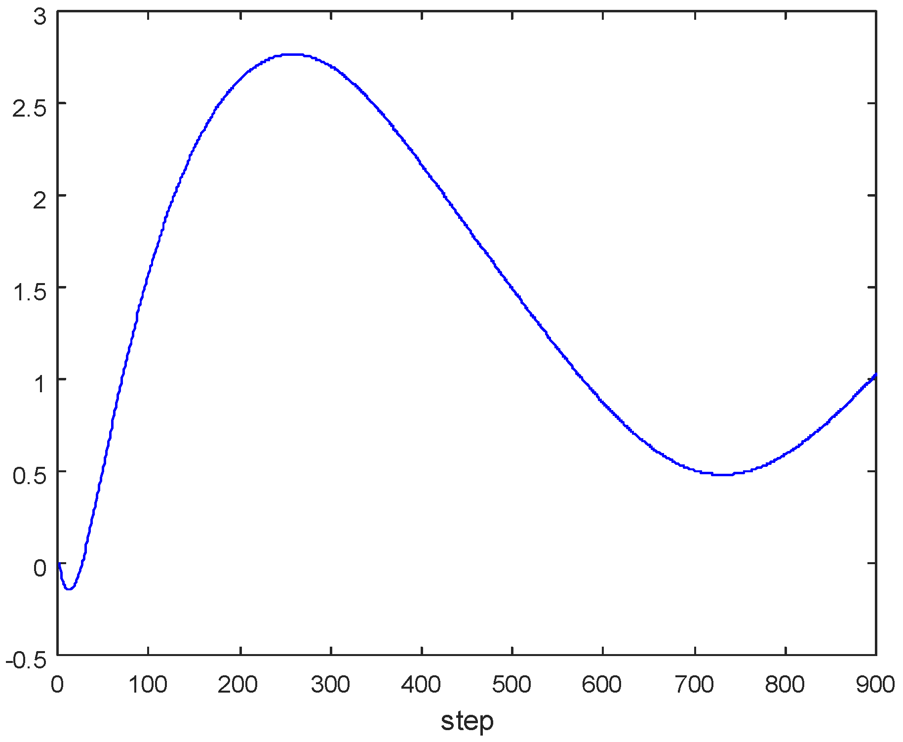
This step results in a 9th order model, which yields numerical errors during the closed-loop simulation. Simulation of transfer function T ( s ) for 1800 s (900 steps) is presented in Figure 7.
This example shows that even a correctly executed identification experiment that results in mathematically correct SISO models may eventually lead to a situation in which the internal model is incorrect due to the effects of the high order model. The model’s irregularities result from numerical problems and are visible only during simulation of the model in the GPC internal model format. This unfavorable property must be correctly identified at the stage of synthesis of the control algorithm. In the event of this unfavorable situation, appropriate remedial measures must be taken. Otherwise, the overall control performance will be negatively impacted, and the closed loop response of the resulting predictive controller may be unstable. This situation is showed in the next simulation.
The resulting GPC controller, with the 9th order internal model, was simulated in closed loop and the three individual modes, before the reduction to common denominator, were used as the plant. The results of the simulation are shown in Figure 8 and Figure 9. As can be easily seen, the control signals are not smooth, resulting from numerical issues. The same experiment was repeated with larger values in the MV penalty matrix R with similar results. The poor performance is caused by numerical issues associated with the simulation using a high order internal model of the GPC controller. Furthermore, the addition of another input further increases the transfer function order and leads to complete destabilization of the algorithm in closed loop.
The problem outlined above can be solved in several ways. The methods of model order reduction may be considered as the first solution. Linear systems have seen a wide variety of reduction techniques such as modal/eigenvalue truncation [37], Lyapunov balanced truncation [38], frequency weighted model reduction [39], normalized co-prime factorization [40], moment matching [41], optimal Hankel approximations [42], Karhunen-Loève (proper orthogonal decomposition (POD)) [43], approximation by a lower order time-delay model [44], etc. However, these methods require specialized knowledge in detailed mathematics. In this paper, we strive to find an effective engineering method that can be utilized by engineers and practitioners in the industry.

5. Model Order Reduction Method

The 9th order model that results from combining (13), (14), and (16) to a common denominator can be reduced to a lower order model by utilizing an approximation of the original transfer function. This method is not a mathematically rigorous method, but rather is meant to be a practical method that is based on engineering judgement and simulation. This method may require some trails and error iterations to obtain the desired closed loop response. In this example, each 3rd order SISO model will be approximated independently by a 2nd order SISO model. The approximation is made based on an engineering judgment driven approximation method consisting of removing similar time constants from the nominator and denominator of transfer function or replacing these three-time constants by two slightly bigger ones. The reduced transfer functions are defined by Equations (18), (19), and (20):
T 1 ( s ) = Y ( s ) U 1 ( s ) = 1 ( 120 s 1 ) ( 90 s + 1 ) ( 110 s + 1 )
T 2 ( s ) = Y ( s ) U 2 ( s ) = 1 ( 20 s 1 ) ( 80 s + 1 ) ( 180 s + 1 )
T 3 ( s ) = Y ( s ) U 3 ( s ) = 1 ( 40 s + 1 ) ( 60 s + 1 )
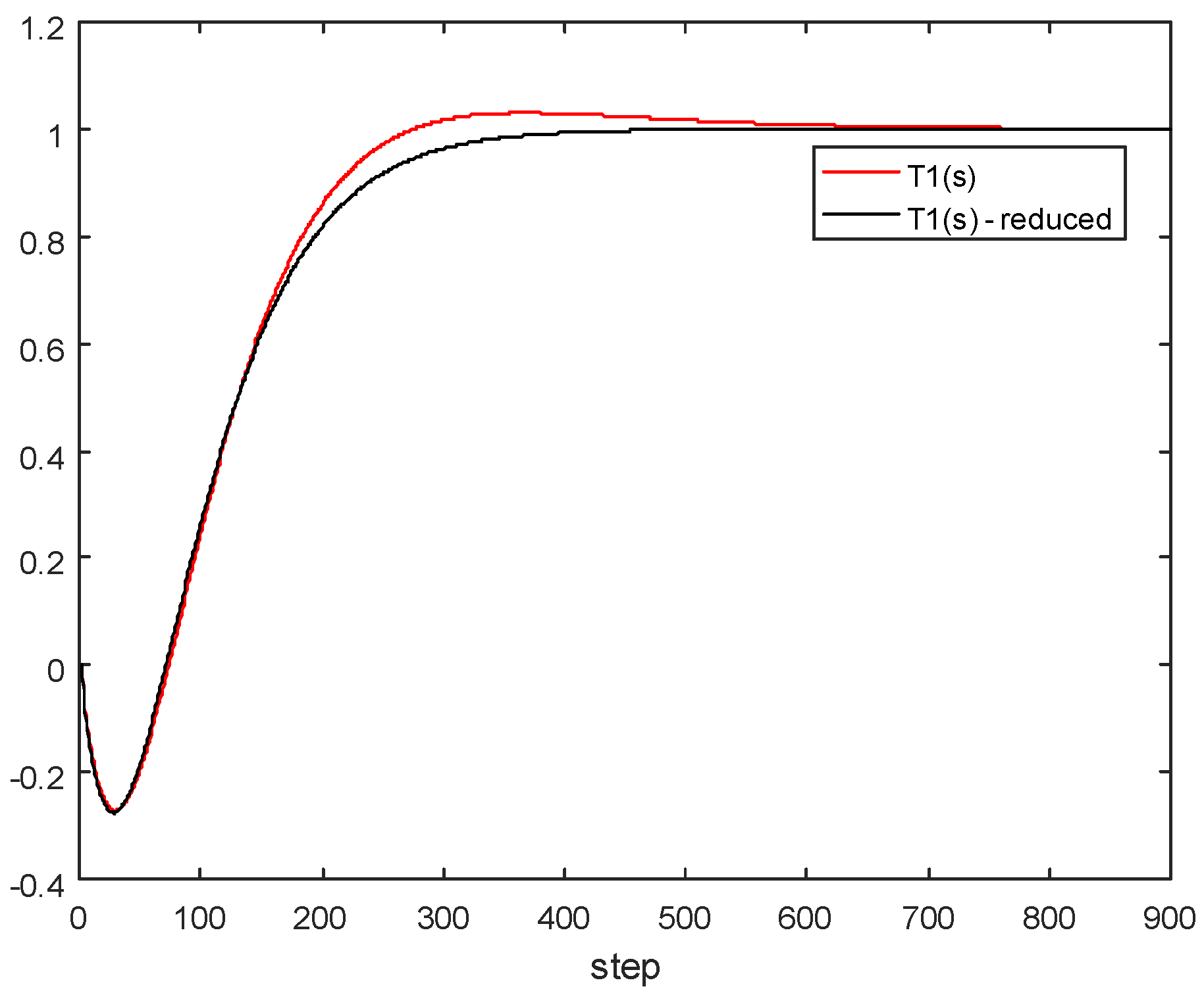
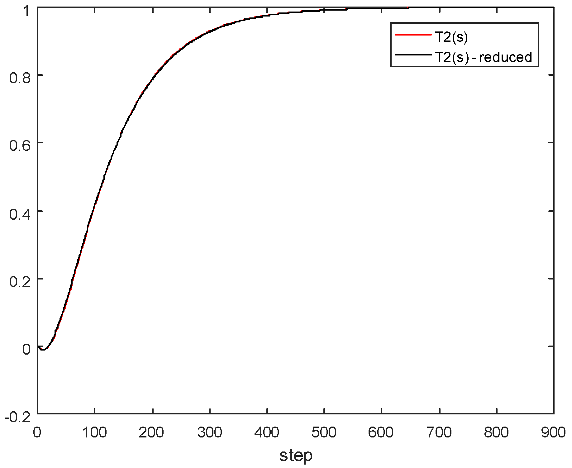
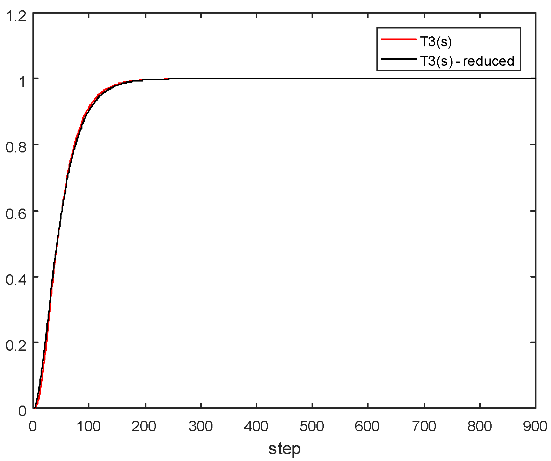
The quality of the model after the order reduction step was verified by simulation. The results are shown in Figure 10, Figure 11 and Figure 12.
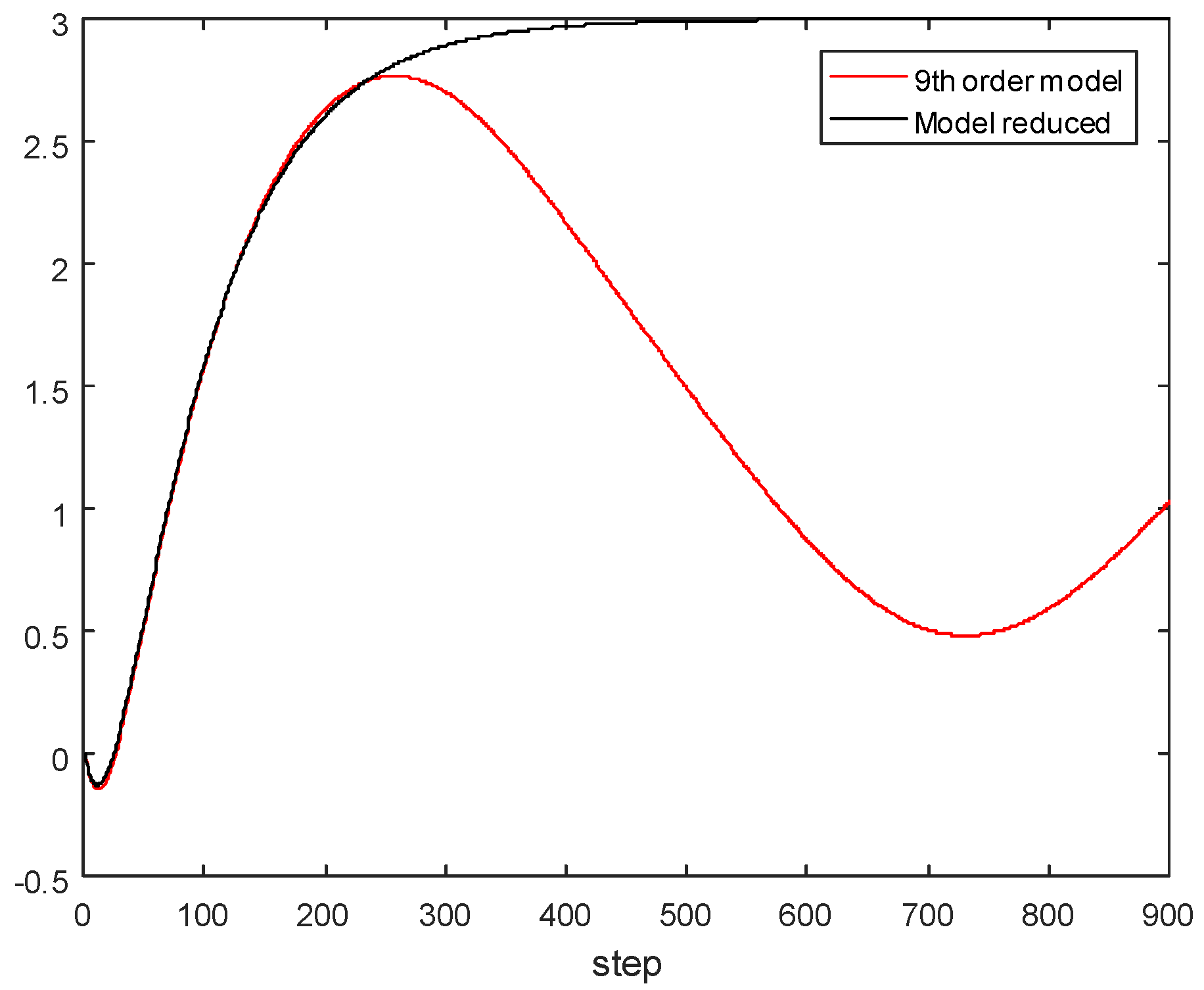
The results of the simulation are very good. In practice, the approximation of the 3rd order model with a 2nd order model usually leads to good results. In the next step, three 2nd order SISO models were reduced to a common denominator and added to meet the requirements for the GPC model form (3). This resulted in a 6th order reduced model and this reduced model is compared with the original 9th order model that was obtained by adding the three original SISO models. The simulations results are shown in Figure 13.
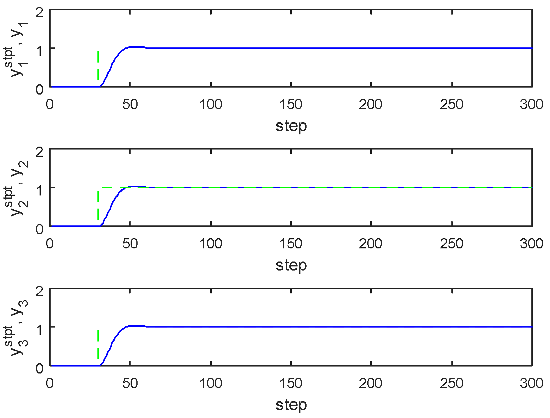
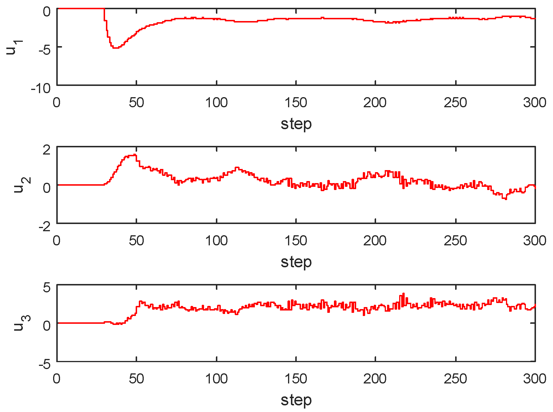
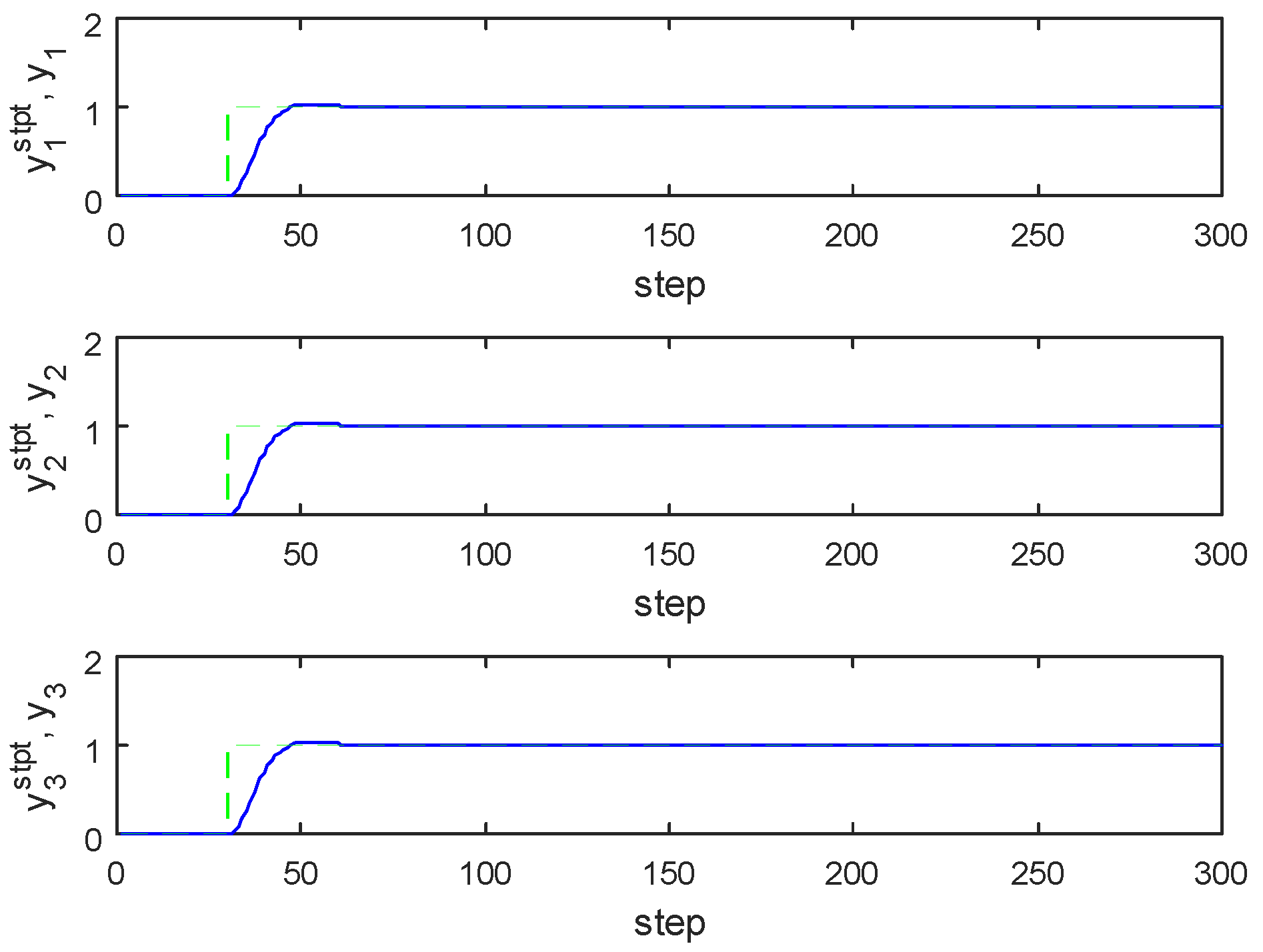
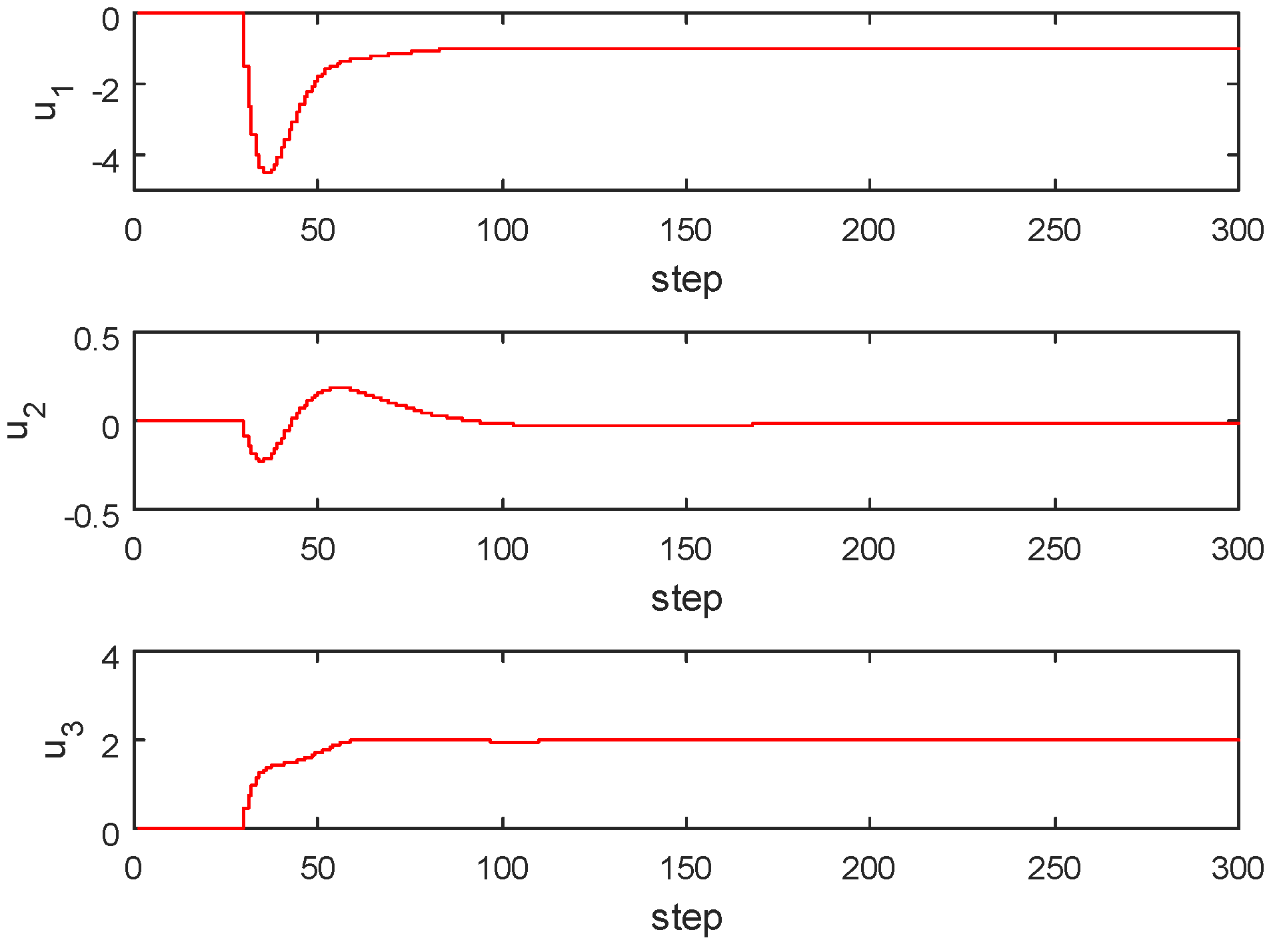
The static gain of the 6th order reduced model is equal to 3 and thus the reduced model compares closely to the expected model. A closed loop simulation of the resulting GPC controller utilizing the reduced order internal model (6th order) was performed and the original 3rd orders models, before reduction to common order given by (13), (14), and (16), were used. The resulting GPC controller was found to be stable through simulation and the results are shown in Figure 14 and Figure 15.

6. Conclusions

The example presented in this article shows that the GPC algorithm applied to MISO objects may be unstable due to numerical problems caused by the high order model. It may be helpful to solve numerical problems of high order models by using an order reduction technique. However, this solution has limitations and may not be effective with models that have a large number of input signals.
In addition to order reduction, this problem can be solved by using longer sampling times. A longer sampling time improves numerical stability, but this approach also has limitations for processes that exhibit fast dynamics. Another solution is to identify the model as a MISO model with a predefined model order instead of identifying the SISO models and changing the model to a common denominator model.
A completely different approach could be to use an estimator to calculate the change in output regardless of each input. This would eliminate the need to reduce the internal model to a common denominator and avoid high order models. Such research goes beyond the framework of this article and may be further investigated.
The problem described for the GPC controller is not applicable to other predictive control structures such as Dynamic Matrix Control (DMC). This is due to the structure of the model, which in the case of the DMC controller is the step response coefficients. Based on our industrial experience of applying GPC, we have found that if the order of the internal model, after the reduction operation, exceeds 9th order, the resulting GPC controller will be subject to numerical issues. In cases where this occurs, we have found that the best course of action is to utilize another control structure such as DMC.
An alternative interesting direction would be to investigate the model predictive controller algorithm, in which the internal model is described by a state space model (MPCs). Checking and comparing the sensitivity of GPC and MPCs algorithms could be an interesting continuation of the problem shown.

Author Contributions

Conceptualization, S.P. and R.W.K.; Validation, R.W.K.; Formal analysis, S.P.; Investigation, S.P.; Writing—original draft preparation, S.P.; Writing—review and editing, R.W.K. All authors have read and agreed to the published version of the manuscript.

Funding

This research received no external founding.

Conflicts of Interest

The authors declare no conflict of interest.

Abbreviations

The following abbreviations are used in this manuscript
GPCGeneralized Predictive Control
MPCModel Predictive Control
PIDProportional, Integral and Derivative
MIMOMultiple-Input Multiple-Output
SISOSingle-Input Single-Output
DCSDistributed Control system
PLCProgrammable Logic Controllers
FPGAField Programmable Gate Arrays
MVManipulated Variable
CVControlled Variable
DVDisturbance Variable
CRHPCConstrained Receding Horizon Predictive Control
SIORHCStabilizing Input Output Receding Horizon Control
QPQuadratic Programming
CPUCentral Processing Unit

References

  1. Camacho, E.F.; Bordons, C. Model Predictive Control; Springer: London, UK, 1999. [Google Scholar]
  2. Ławryńczuk, M. Computationally Efficient Model Predictive Control Algorithms: A Neural Network Approach, Studies in Systems, Decision and Control; Springer International Publishing: Cham, Switzerland, 2014; Volume 3. [Google Scholar]
  3. Qin, S.J.; Badgwell, T.A. A survey of industrial model predictive control technology. Control Eng. Pract. 2003, 11, 733–764. [Google Scholar] [CrossRef]
  4. Domański, P. Performance Assessment of Predictive Control—A Survey. Algorithms 2020, 13, 97. [Google Scholar] [CrossRef] [Green Version]
  5. El Youssef, J.; Castle, J.; Ward, W.K. A Review of Closed–Loop Algorithms for Glycemic Control in the Treatment of Type 1 Diabetes. Algorithms 2009, 2, 518–532. [Google Scholar] [CrossRef] [Green Version]
  6. Sands, T. Comparison and Interpretation Methods for Predictive Control of Mechanics. Algorithms 2019, 12, 232. [Google Scholar] [CrossRef] [Green Version]
  7. Forbes, M.G.; Patwardhan, R.; Hamadah, H.; Gopaluni, R. Model predictive control in in-dustry: Challenges and opportunities. IFAC PapersOnLine 2015, 48, 531–538. [Google Scholar] [CrossRef]
  8. Marusak, P.; Kuntanapreeda, S. A neural network-based implementation of an MPC algorithm applied in the control systems of electromechanical plants. In Proceedings of the 8th TSME–International Conference on Mechanical Engineering (TSME–ICoME), Bangkok, Thailand, 12–15 December 2017. [Google Scholar]
  9. Abdelaal, M.; Schön, S. Predictive Path Following and Collision Avoidance of Autonomous Connected Vehicles. Algorithms 2020, 13, 52. [Google Scholar] [CrossRef] [Green Version]
  10. Marusak, P. Numerically Efficient Fuzzy MPC Algorithm with Advanced Generation of Prediction—Application to a Chemical Reactor. Algorithms 2020, 13, 143. [Google Scholar] [CrossRef]
  11. Wu, X.; Shen, J.; Li, Y.; Lee, K.Y. Fuzzy modeling and predictive control of superheater steam temperature for power plant. ISA Trans. 2015, 56, 241–251. [Google Scholar] [CrossRef]
  12. Khooban, M.H.; Vafam, N.; Niknam, T. Optimal partitioning of a boiler–turbine unit for Fuzzy model predictive control. ISA Trans. 2016, 64, 231–240. [Google Scholar] [CrossRef]
  13. Kong, L.; Yuan, J. Disturbance–observer–based fuzzy model predictive control for nonlinear processes with disturbances and input constraints. ISA Trans. 2019, 90, 74–88. [Google Scholar] [CrossRef]
  14. Kong, L.; Yuan, J. Generalized Discrete–time Nonlinear Disturbance Observer Based Fuzzy Model Predictive Control for Boiler–Turbine Systems. ISA Trans. 2019, 90, 89–106. [Google Scholar] [CrossRef] [PubMed]
  15. Shen, D.; Lim, C.-C.; Shi, P. Robust fuzzy model predictive control for energy management systems in fuel cell vehicles. Control Eng. Pract. 2020, 98, 104364. [Google Scholar] [CrossRef]
  16. Killian, M.; Kozek, M. T–S fuzzy model predictive speed control of electrical vehicles. IFAC PapersOnLine 2017, 50, 2011–2016. [Google Scholar] [CrossRef]
  17. Marusak, P.; Tatjewski, P. Stability analysis of nonlinear control systems with unconstrained fuzzy predictive controllers. Arch. Control Sci. 2002, 12, 267–288. [Google Scholar]
  18. Boulkaibet, I.; Belarbi, K.; Bououden, S.; Marwala, T.; Chadli, M. A new T–S fuzzy model predictive control for nonlinear processes. Expert Syst. Appl. 2017, 88, 132–151. [Google Scholar] [CrossRef]
  19. Essien, E.; Ibrahim, H.; Mehrandezh, M.; Idem, R. Adaptive neuro-fuzzy inference system (ANFIS)—Based model predictive control (MPC) for carbon dioxide reforming of methane (CDRM) in a plug flow tubular reactor for hydrogen production. Therm. Sci. Eng. Prog. 2019, 9, 148–161. [Google Scholar] [CrossRef]
  20. Wojtulewicz, A.; Ławryńczuk, M. Computationally efficient implementation of dynamic matrix control algorithm for very fast processes using programmable logic controller. In Proceedings of the 23th IEEE International Conference on Methods and Models in Automation and Robotics (MMAR 2018), Międzyzdroje, Poland, 27–30 August 2018; pp. 579–584. [Google Scholar]
  21. Plamowski, S. Implementation of DMC algorithm in embedded controller—Resources, memory and numerical modifications. In Proceedings of the KKA 2017—The 19th Polish Control Conference, Kraków, Poland, 18–21 June 2017; pp. 335–343. [Google Scholar]
  22. Chaber, P.; Ławryńczuk, M. Fast analytical model predictive controllers and their implementation for STM32 ARM microcontroller. IEEE Trans. Ind. Inform. 2019, 15, 4580–4590. [Google Scholar] [CrossRef]
  23. Wojtulewicz, A.; Ławryńczuk, M. Implementation of Multiple-Input Multiple-Output Dynamic Matrix Control Algorithm for Fast Processes Using Field Programmable Gate Array. In Proceedings of the 15th IFAC Conference on Programmable Devices and Embedded Systems PDeS, Ostrava, Czech Republic, 23–25 May 2018; pp. 324–329. [Google Scholar]
  24. Morari, M.; Lee, J.H. Model predictive control: Past, present and future. Comput. Chem. Eng. 1999, 23, 667–682. [Google Scholar] [CrossRef]
  25. Salez, D.; Cipriano, A.; Ordys, A.W. Optimisation of Industrial Processes at Supervisory Level; Springer: London, UK, 2002. [Google Scholar]
  26. Tatjewski, P. Advanced Control of Industrial Processes; Springer: London, UK, 2007. [Google Scholar]
  27. Findeisen, W. Control and Coordination in Hierarchical Systems, Chichester (Eng.); John Wiley & Sons: New York, NY, USA, 1980. [Google Scholar]
  28. Kayacan, E.; Peschel, J. Robust Model Predictive Control of Systems by Modelling Mismatched Uncertainty. IFAC-PapersOnLine 2016, 49, 265–269. [Google Scholar] [CrossRef]
  29. Plamowski, S.; Tatjewski, P. Safe implementation of advanced control in a diagnostic-based switching structure. In Proceedings of the 6th IFAC Symposium on Fault Detection, Supervision and Safety of Technical Processes, Beijing, China, 30 August–1 September 2006; pp. 487–495. [Google Scholar]
  30. Clarke, D.W.; Mohtadi, C.; Tuffs, S. Generalized predictive control—Parts I and II. Automatica 1987, 23, 137–160. [Google Scholar] [CrossRef]
  31. Clarke, D.W.; Mohtadi, C. Properties of generalized predictive control. Automatica 1989, 25, 859–875. [Google Scholar] [CrossRef]
  32. Gorez, R.; Wertz, V.; Zhu, K.Y. On a generalised predictive control algorithm. Syst. Control Lett. 1987, 9, 369–377. [Google Scholar] [CrossRef]
  33. Grimble, M.J. Generalized predictive optimal control: An introduction to the advantages and limitations. Int. J. Syst. Sci. 1992, 23, 85–98. [Google Scholar] [CrossRef]
  34. Clarke, D.W.; Scattolini, R. Constrained receding-horizon predictive control. IEE Proc. D 1991, 138, 347–354. [Google Scholar] [CrossRef]
  35. Bemporad, A.; Chisci, L.; Mosca, E. On the stabilizing property of SIORHC. Automatica 1994, 30, 2013–2015. [Google Scholar] [CrossRef]
  36. Maciejowski, J.M. Predictive Control with Constraints; Prentice Hall: London, UK, 2002. [Google Scholar]
  37. Hughes, P.C.; Skelton, R. Modal truncation for flexible spacecraft. J. Guid. Control 1981, 4, 291–297. [Google Scholar]
  38. Moore, B. Principal component analysis in linear systems: Controllability, observability, and model reduction. IEEE Trans. Autom. Control 1981, 26, 17–32. [Google Scholar] [CrossRef]
  39. Enns, D. Model reduction with balanced realizations: An error bound and a frequency weighted generalization. In Proceedings of the 23rd IEEE Conference on Decision and Control, Las Vegas, NV, USA, 12–14 December 1984; Volume 23, pp. 127–132. [Google Scholar]
  40. Anderson, B.; Liu, Y. Controller reduction: Concepts and approaches. IEEE Trans. Autom. Control 1989, 34, 802–812. [Google Scholar] [CrossRef]
  41. Astolfi, A. Model Reduction by Moment Matching for Linear and Nonlinear Systems. IEEE Trans. Autom. Control 2010, 55, 2321–2336. [Google Scholar] [CrossRef]
  42. Glover, K. All optimal Hankel-norm approximations of linear multivariable systems and their L∞-error bounds. Int. J. Control 1984, 39, 1115–1193. [Google Scholar] [CrossRef]
  43. Willcox, K.; Peraire, J. Balanced model reduction via the proper orthogonal decomposition. AIAA J. 2002, 40, 2323–2330. [Google Scholar] [CrossRef]
  44. Kubalčik, M.; Bobál, V. Predictive control of higher order systems approximated by lower order time-delay models. WSEAS Trans. Syst. 2012, 11, 607–616. [Google Scholar]
Figure 1. MISO model as a set of SISO models.
Algorithms 13 00178 g001
Figure 2. Step response for T1 and T2 transfer functions simulated for 900 time-steps.
Algorithms 13 00178 g002
Figure 3. Step response of the 6th order model after reduction to a common denominator simulated for 900 time-steps.
Algorithms 13 00178 g003
Figure 4. GPC with the 6th order internal model—closed loop simulation of 300 time-steps, dashed line is the set point, and the solid line is the CV.
Algorithms 13 00178 g004
Figure 5. GPC with the 6th order internal model—closed loop simulation of 300 time-steps, trend for MVs signals.
Algorithms 13 00178 g005
Figure 6. Step response for T1, T2, and T3 transfer functions simulated for 900 time-steps.
Algorithms 13 00178 g006
Figure 7. Step response of the 9th order model after reduction to common denominator simulated for 900 time-steps.
Algorithms 13 00178 g007
Figure 8. GPC with the 9th order internal model—closed loop simulation of 300 time-steps; dashed line is a set point, solid is a CV, and control parameters as: control horizon N u = 20 , prediction horizon N = 400 , and the R matrix = identity matrix.
Algorithms 13 00178 g008
Figure 9. GPC with the 9th order internal model—closed loop simulation of 300 time-steps, trend for MVs signals. Controller parameters: control horizon N u = 20 , prediction horizon N = 400 , and the R matrix = identity matrix.
Algorithms 13 00178 g009
Figure 10. Comparison of original and T1 and after order reduction (black line)—simulation of 900 time-steps.
Algorithms 13 00178 g010
Figure 11. Comparison of original and T2 and after order reduction (black line)—simulation of 900 time-steps.
Algorithms 13 00178 g011
Figure 12. Comparison of original and T3 and after order reduction (black line)—simulation of 900 time-steps.
Algorithms 13 00178 g012
Figure 13. Comparison of the 6th and 9th order models—simulation of 900 time-steps (solid line—9th order model, dashed line—6th order model—model after order reduction).
Algorithms 13 00178 g013
Figure 14. GPC with reduced internal model—closed loop simulation of 300 time-steps where the dashed line is the set point and the solid line is the CV. Controller parameters: control horizon N u = 20 , prediction horizon N = 400 , and the R matrix = identity matrix.
Algorithms 13 00178 g014
Figure 15. GPC with reduced internal model closed loop simulation of 300 time-steps, trend for MVs signals (u1, u2 and u3). Controller parameters: control horizon N u = 20 , prediction horizon N = 400 , and the R matrix = identity matrix.
Algorithms 13 00178 g015