Abstract
Bayesian Networks (BN) are probabilistic models that are commonly used for the diagnosis in numerous domains (medicine, finance, transport, robotics, …). In the case of autonomous vehicles, they can contribute to elaborate intelligent monitors that can take the environmental context into account. We show in this paper some main abilities of BN that can help in the elaboration of fault detection isolation and recovery (FDIR) modules. One of the main difficulty with the BN model is generally to elaborate these ones according to the case of study. Then, we propose some automatic generation techniques from failure mode and effects analysis (FMEA)-like tables using the pattern design approach. Once defined, these modules have to operate online for autonomous vehicles. In a second part, we propose a design methodology to embed the real-time and non-intrusive implementations of the BN modules using FPGA-SoC support. We show that the FPGA implementation can offer an interesting speed-up with very limited energy cost. Lastly, we show how these BN modules can be incorporated into the decision-making model for the mission planning of unmanned aerial vehicles (UAVs). We illustrate the integration by means of two models: the Decision Network model that is a straightforward extension of the BN model, and the BFM model that is an extension of the Markov Decision Process (MDP) decision-making model incorporating a BN. We illustrate the different proposals with realistic examples and show that the hybrid implementation on FPGA-SoC can offer some benefits.
1. Introduction
Bayesian Networks (BNs) are well known probabilistic models to elaborate diagnosis taking into account uncertainties. Numerous fields of applications like medicine, robotics, industrial process, exploit their inference mechanism to evaluate the causes of a disease or the source of the malfunctioning from the observed environment. With the autonomy of unmanned aerial vehicles (UAV), the safety becomes a major issue to achieve the mission correctly. Then the analysis and the evaluation of the dependability of the system [1] including the safety and the security constraints are crucial. In the case of aerospace systems, a set of faults and errors [2] related to sensors, actuators and embedded systems can be identified in advance. To detect and to mitigate the different kinds of hazards, number of model-based fault detection isolation recovery (FDIR) techniques have been introduced [3].
The BNs are used in safety and risk analysis/assessment. The superiority of the BN over conventional risk analysis methods such as the Bowtie method and Fault tree are well proven in many literatures [4,5,6]. In [7,8,9], the FDIR techniques use static or dynamic BNs in order to define the Health Management (HM) of the system from sensor observation. Other works [10,11] in security show that BNs can be also used to model particular security threats. The BN model can be an interesting model for elaborating intelligent monitors for autonomous vehicles.
The elaboration of the appropriate BN able to fit the dependable system is a complex task and is generally based on expert knowledge or on the learning algorithms [12,13,14]. Learning algorithms can help in defining the parameters and the structure of the networks. Nevertheless, they are really inefficient if not driven by some expertise. The first challenge is then to elaborate these ones without being a BN expert and without using extensive and inefficient learning methods.
The second challenge in the context of autonomous vehicle is to embed these intelligent monitors in the real-time context. Actual UAV systems have the opportunity to embed parallel application by deploying them onto specific parallel architecture such as multi-core CPU, GPU or FPGA architecture. These hardware supports are currently proposed for the real-time vision application [15]. The BN monitors can be described in a parallel way and can be efficiently implemented on FPGA support. A hardware implementation on FPGA of the HM is proposed to achieve real-time objectives and non intrusive monitoring [16,17]. The efficiency of their FPGA implementation relies on the Arithmetic Circuit (AC) compilation [18], proposed for the BN inference, which gives a linear time computational complexity for real-time execution. The main challenge considering this kind of implementation is the design tool/methodology for an easy and a scalable FPGA implementation.
When embedded real-time BN estimators/monitors are available, the next step is to incorporate them into the decision-making module for an operational mission planning. For the mission planning, there are different decision-making models that can be compatible with the BN monitors such as Decision Networks (DN), Markov Decision Process (MDP), POMDP, …As Decision Networks is an extension of BN, the integration of BN monitors to this model is straightforward. For MDP model, the BNs can be used for the transition function between states. The interaction between the BN diagnosis and the decision-making model in the context of the mission management can be challenging in terms of functional distribution and operative organization onto the system.
In this paper, we propose to respond to the three following challenges during elaborating the intelligent estimators/monitors based on BN:
- a simple (friendly) way to generate their BN specifications
- a design methodology to elaborate the efficient BN implementation on parallel FPGA support
- a practical way to incorporate the BN monitors into the decision-making mechanism for the mission management of an autonomous vehicle.
Compared to the literature, our proposal shows different advantages at different levels. At the model level, we propose different BN structures to define the diagnosis and the error mitigation modules. These models can be easily elaborated from FMEA-like tables using design pattern techniques. The BN models and the way to specify them present an advantage compared to [7,8] where the BNs are only elaborated by expertise. Our proposal does not need any BN expertise. This paper proposes also a design methodology to implement the BN monitors onto FPGA. The main advantage of this methodology compared to the literature is a proposal of a complete design flow from FMEA-like tables towards FPGA support. In [10], a dedicated FPGA tool is proposed but does not take as input high-level specifications such as FMEA-tables and does not propose a complete design flow. To elaborate efficient implementations, we also propose specific and original optimizations for the BN structures that can be applied in a systematic way. The last point concerned the BN integration into a decision-making engine. In [9], the authors use Decision Networks to express the mission planning but no systematic method to elaborate them is proposed. In this paper, a methodology to design Decision Networks for the mission planning is presented and it can be extended to other models based on MDP. This methodology offers an easy way to specify the mission that can incorporate BN monitors, no equivalent methodology is proposed in the literature. The disadvantage of this methodology is that it is limited to some patterns that we have selected and it does not take into account for now the historical variations of the evidence to make some predictions or to reinforce the value of the diagnosis. To validate the monitors and the mission planning elaborated by our methodology, we present different study cases that show also the scalability of our proposal.
In Section 2, we focus on some BN models for the diagnosis and the error mitigation. These ones can help to elaborate monitors for some physical or functional elements of the system such as sensors and applications. In Section 3, we focus on the methodology to automatically build these BN monitors from FMEA-like tables and on the methodology to generate an embedded real-time version onto FPGA. Section 4 shows how to incorporate them into a global view of decision-making for the case of the mission management of an autonomous vehicle. This integration is proposed using two possible decision-making models: DN model and MDP model. In Section 5, we show through examples that the BN implementations onto FPGA are efficient and low-power and present some co-design experiment for decision-making modules incorporating BN monitors at the mission management level. Section 6 opens a discussion on the BN parameters and on the cooperation between the diagnosis and decision-making modules at the mission management level.
2. BN Model for the Monitoring and the Error Recovery
In this section, we present different BN models and we show their ability to diagnose and to mitigate errors. We mainly propose some dedicated BN structures. We mention in the last part (Section 6.1) how the parameters of the BN structures can be defined.
2.1. Diagnosis with BN
BNs are probabilistic graphical models used to understand and control the behavior of systems [19]. The nodes of such a network represent random variables, the conditional probabilities of which are given by probability tables (CPTs). The arcs of the network indicate the conditional dependencies. The structure of the Bayesian network is defined by the nodes and the arcs of the corresponding graph. The parameters of the BN are the CPT of the nodes. A simple example of a BN is given in Figure 1. The node UAV Altitude () represents the altitude status describing whether the altitude of the UAV is increasing or decreasing. The nodes Barometer () and Altimeter () represent the sensors observing whether the UAV moves up or down. The node influences the sensor readings, hence there are arcs from to and . The CPT tables for the sensor (), for example, should be read as follows: if the status is “increasing”, then the probability that it is reading an increasing value is .
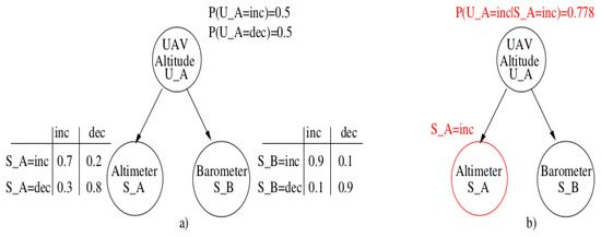
Figure 1.
(a) Definition of a BN with its parameters (CPTs); (b) Illustration of the inference mechanism.
The diagnosis is obtained by using an inference mechanism based on observations on or , and to compute the posterior probabilities over A using Bayes’ theorem (Equation (1)).
We use Bayes’ theorem for our example as follows (Equation (2)):
So with the evidence on , we can say that the probability of the altitude status to be “increasing” equals as shown in Figure 1b. If for example, we add observations on the barometer giving an increasing value, the probability increases to .
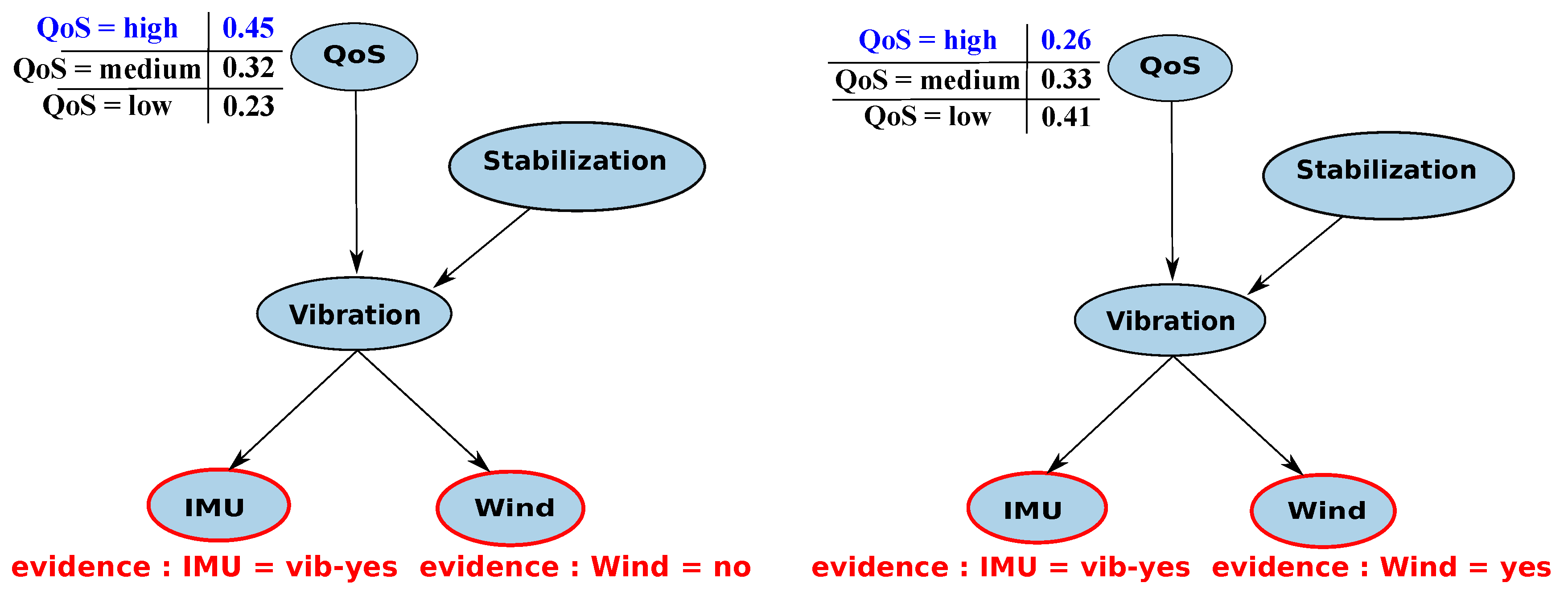
During UAV missions, the evaluation of health status of the components of the system (i.e., sensors, actuators, etc.) is done from sensor data [20]. On the other hand, the Quality of Service (QoS) status of the applications which are executed on board, such as tracking application, can also be monitored to ensure mission success. Figure 2 illustrates the monitoring of the tracking application. For this application, we enumerate the different potential problems that can occur. In this example, one of potential problem is the vibration that can affect the quality of the tracking. The vibration can occur when IMU shows deviation or when strong wind is detected. This BN evaluates the QoS of the application based on evidence on IMU deviation or on wind detection as described in Figure 3.

Figure 2.
BN for vibration error type.
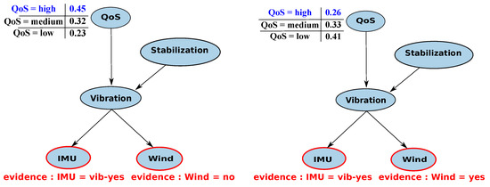
Figure 3.
Application Quality of Service (QoS) probability under the observed context.
2.2. Error Mitigation with BN
BN can also help to mitigate error by proposing the most adequate solution when an error is detected. In this case, the BN includes the potential mitigation proposal. We fix the expected resultant and we calculate by inference the most adequate solution to solve the problem. To ensure the quality of service of the application, some error recovery can be activated. In that case, if we activate the stabilization, the QoS of the application increases. To know if it is useful to activate the stabilization, we can proceed by inference. We evaluate the probability to activate the stabilization by fixing the quality of service at high. If this probability is high that means that the most appropriate action is to activate the stabilization in order to increase the QoS. This principle is illustrated in Figure 4.

Figure 4.
The probability to activate is the stabilization to maintain a good QoS of the application depending on the evidence on IMU and wind.
2.3. Integration of the Embedded System Constraints
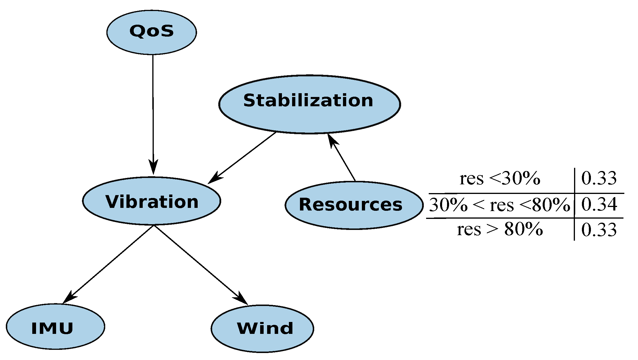
In the context of embedded systems, the constraints related to the system cannot be ignored. It is important to capture these system constraints and to integrate them at the monitor level for considering a realistic solution. The system constraints include resource constraints, timing constraints and the energy consumption ones. The resource constraints of the vibration example can be associated to the application as shown in Figure 5.

Figure 5.
BN for Vibration Including Resource Constraint.
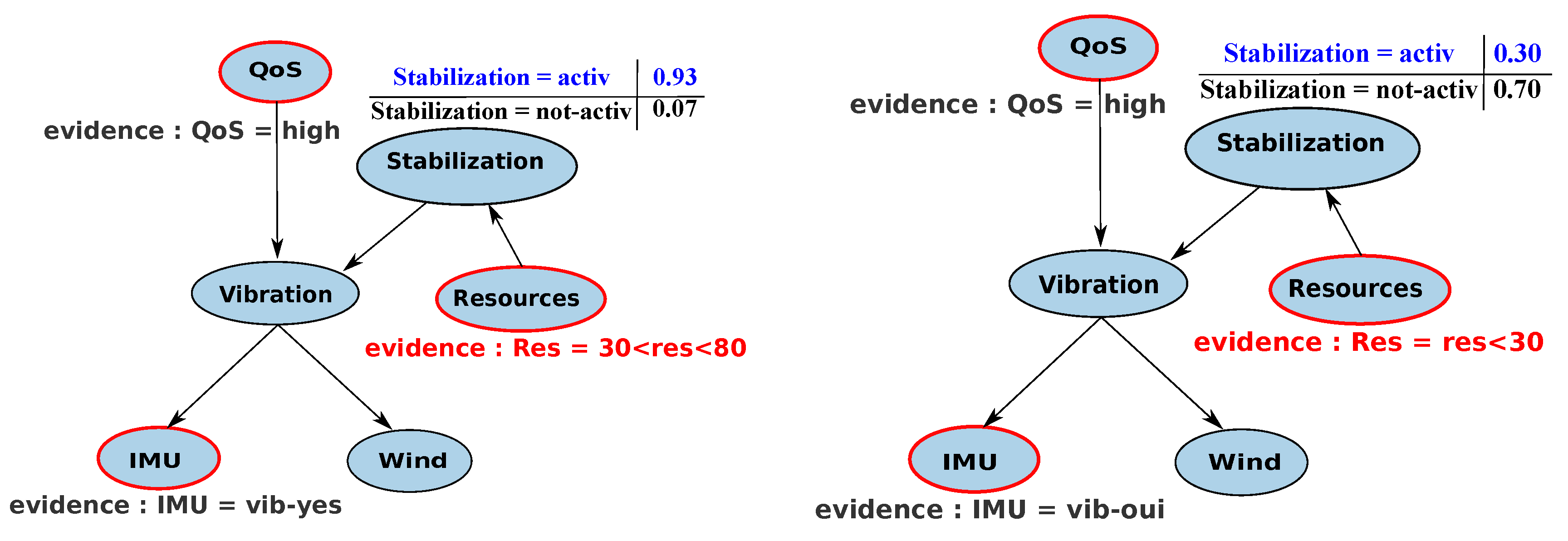
We show in Figure 6 that depending on resource availability, we can choose to activate the stabilization for the application (case when resource >30%) or not if there are not enough resources available (case resource <30%).
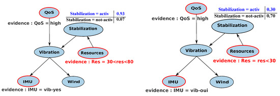
Figure 6.
Choice of the solution (error mitigation) adapted to the resources availability using BN.
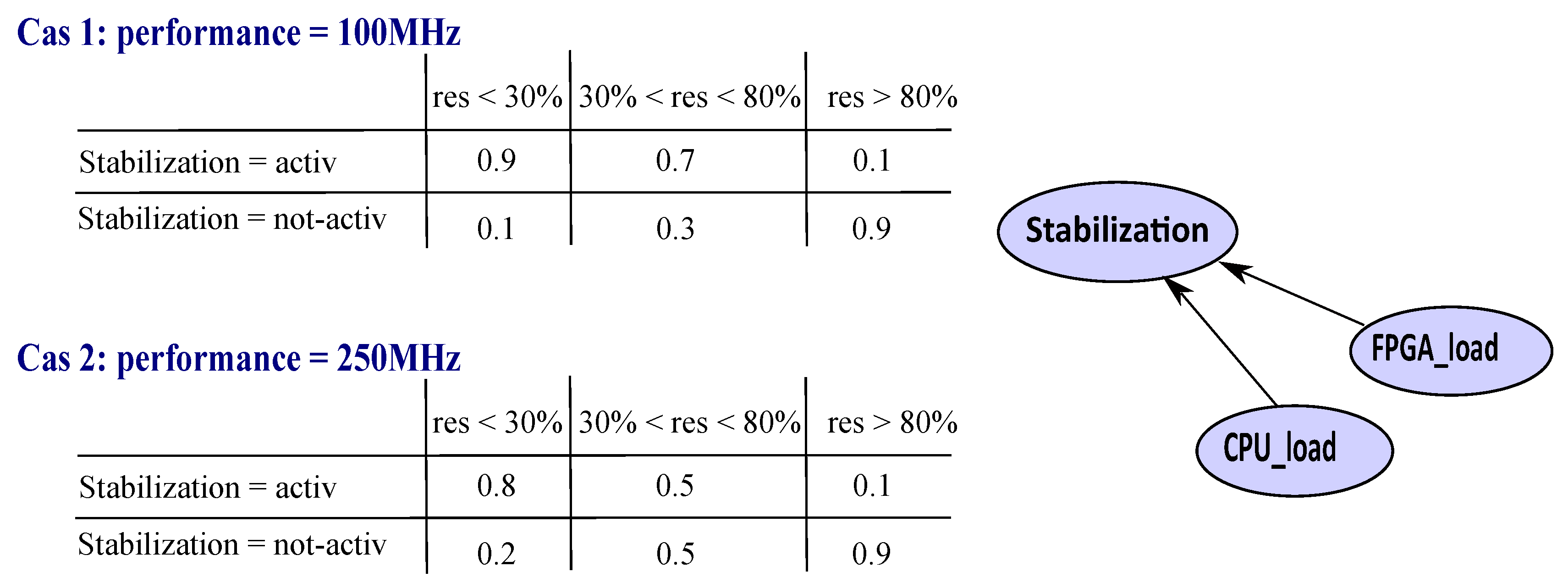
The timing constraints can be inserted also in the BN model, connected to the resource information. Actually, the resource needed for the application implementation can increase to provide an application with a better performance because parallel functions need generally more resource to operate in a parallel way. This can be modeled with the parameters of the BN model as shown in Figure 7. To operate at 250 MHz, we need more resources (>30%) than if we operate at 100 MHz.
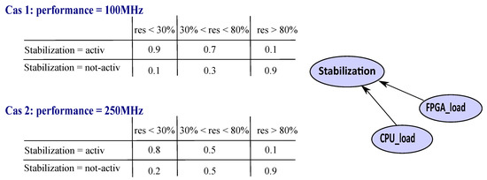
Figure 7.
Integration of the performances in the initial probability table.
A BN model for HM specifications allows to take into account the uncertainty of the context of the mission, based on sensor information. Nevertheless, for a non-expert in BN models, the HM specifications for diagnosis or error mitigation are not so easy to elaborate. We propose in the next section to simplify the specifications of HM by catching the main error contexts, the main systems constraints and main mitigation solutions by means of simple FMEA-like tables. These tables enable to define the underlying BN models based on a pattern driven approach.
3. Methodology for an Automatic BN Generation and Its Embedded Implementation
The specific structures of BN able to specify the monitors and the error recovery can be defined automatically from FMEA-like table using pattern driven approach. The embedded version of these BN monitors necessitate to elaborate new design tools to implement them onto FPGA. We propose a complete design flow from FMEA-tables towards FPGA implementation dedicated to the BN monitors.
3.1. Pattern Driven Approach
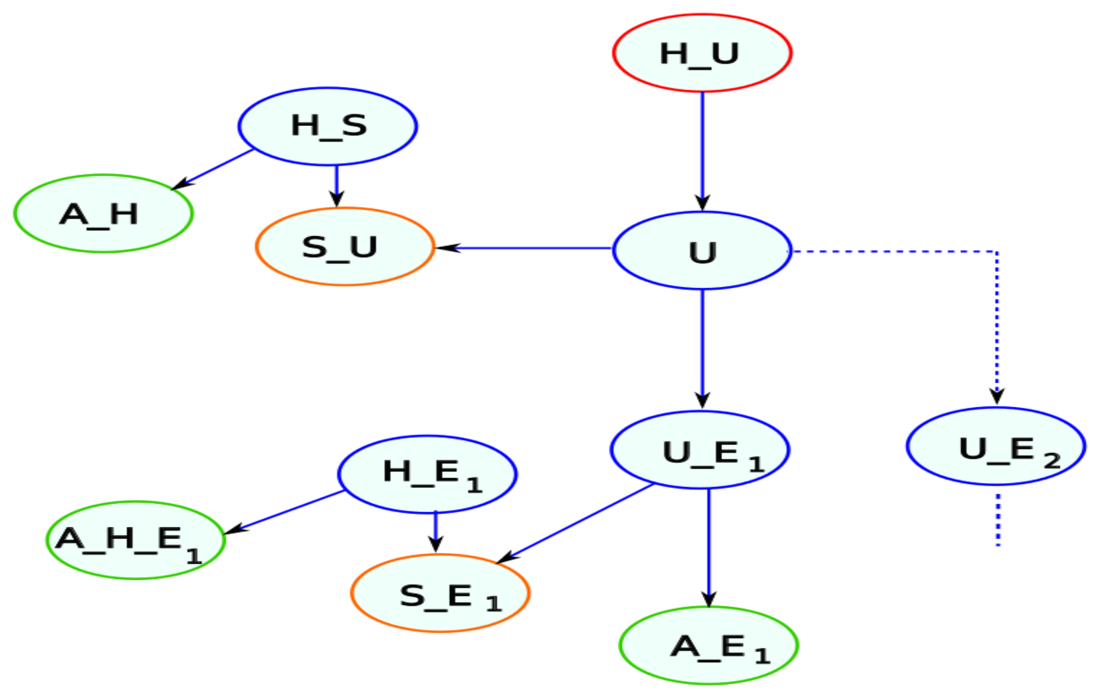
We define different patterns that can introduce the environment constraints, the system constraints, the application constraints and the possible mitigations. Patterns represent some specific structures of BN that can be elaborated from FMEA-like tables. Here we list the three main patterns: the pattern, the pattern and the pattern, respectively representing the context-aware diagnosis, the error mitigation proposal with or without the embedded constraints. These ones are detailed below.
3.1.1. The Pattern
The health status of an element of the system can be defined by the BN structure detailed in Figure 8. If the element U is the element to monitor, we define its health status. Its value depends on the possible types of error that can degrade the functioning of the element and this can happen for some particular appearance contexts. The appearance contexts represent the causes that reinforce the belief of error presence. These types of error can be monitoring using specific sensors that can be faulty themselves. Table 1 summarizes the results of this analysis and defines the main nodes of the BN structure, where each represents an error type, defining source of failure. This error can be monitored by the appearance contexts and/or sensors that can be hardware or software. The sensors can themselves be faulty; information can also be reinforced by the appearance contexts () of the Health status of the sensors (). In addition to error types, we need an internal monitor of the global system (). The information given by the monitor can be reinforced by the appearance contexts () of the Health status of the monitor (). From Table 1 we can automatically generate the BN structure associated to the pattern.
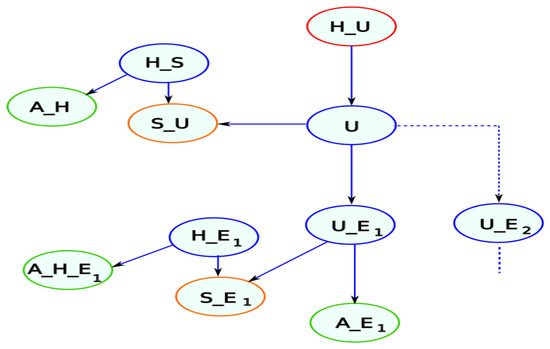
Figure 8.
Failure mode and effects analysis (FMEA)_Health Management (HM) pattern for BN where the , nodes represent the sensor nodes of either a hardware or a software monitor, the nodes U, are the internal states possibly affected by an error , the node represents the health of the system, and nodes represent the health of the sensor and the , are the appearance contexts.

Table 1.
FMEA table for an error type Health Management ( pattern).
3.1.2. The Pattern
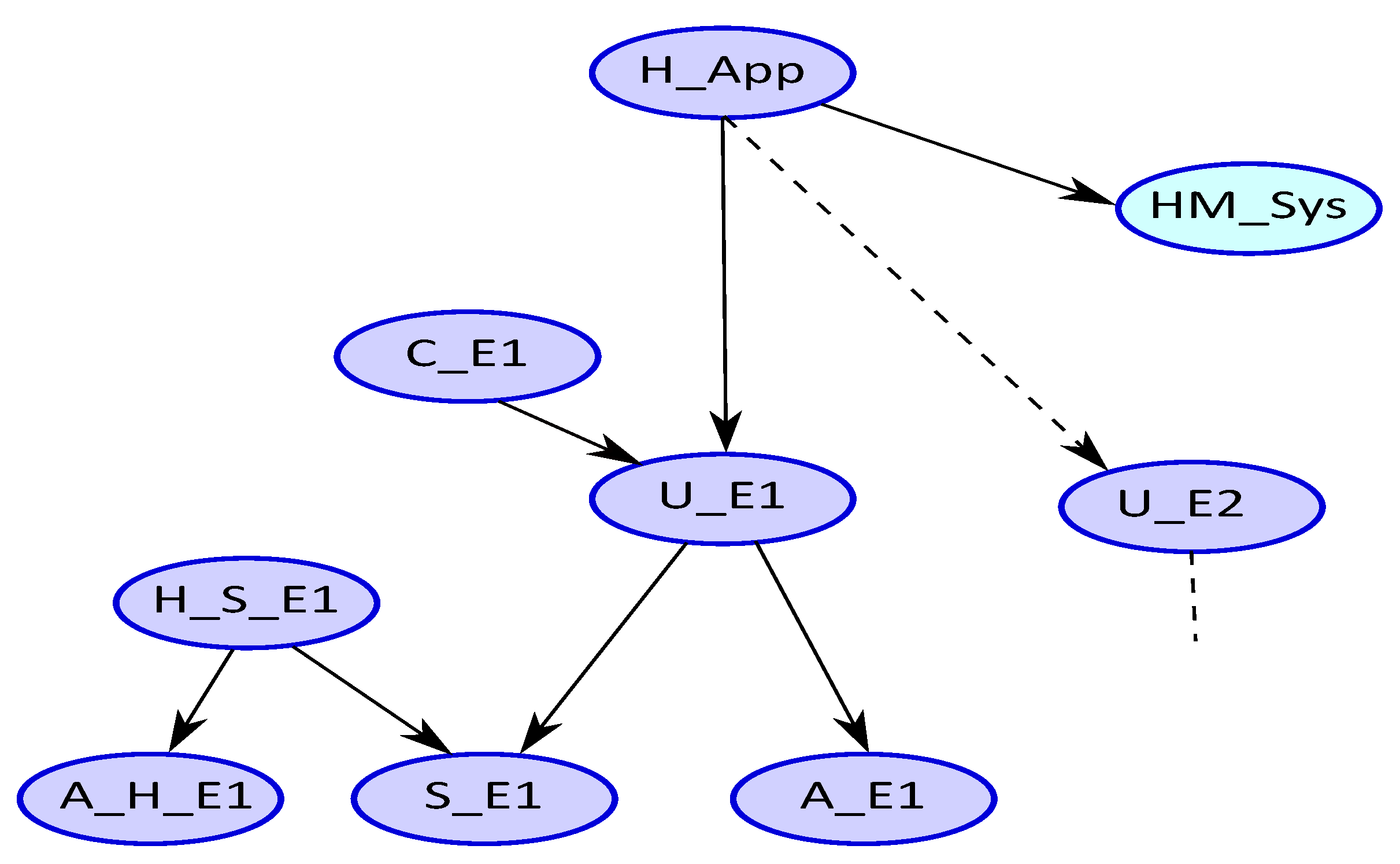
We can include in the previous FMEA-table the possible error mitigation for a specific type of error. This structure is especially useful to propose an alternative for an application. Therefore, this BN computes the health of the application () that represents . A novel column is added and corresponds to the possible mitigation solution for the error type . The new table is shown in Table 2. This table corresponds to the generic BN structure described in Figure 9 that is an extension of . The node HM_Sys represents the Health of the system and can be added in the BN structure as it can be considered as an potential error associated to the system malfunctioning.

Table 2.
FMEA table to mitigate errors ( pattern).
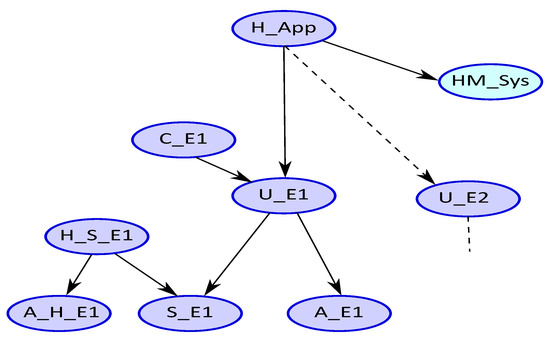
Figure 9.
BN structure associated to pattern where C_Ei represents the error mitigation.
3.1.3. The Pattern
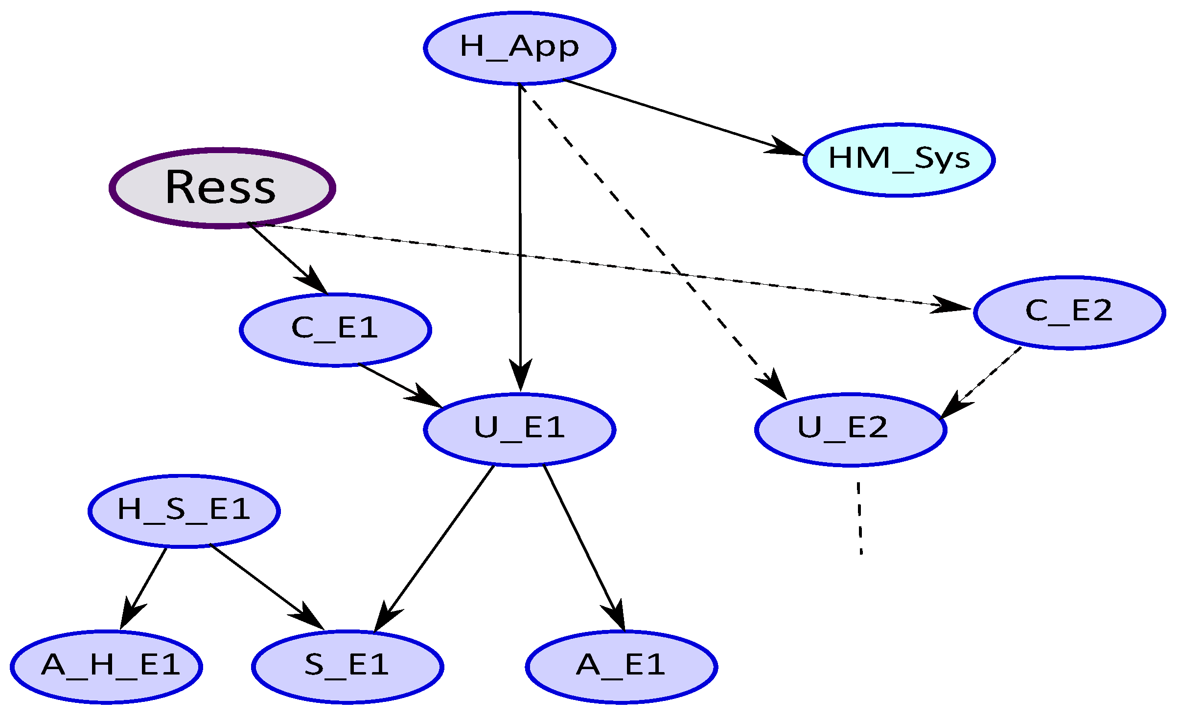
For an embedded application or sensor, it is necessary to respect the timing constraints and resource constraints. These constraints can be added in the same manner into an FMEA-like table as shown in Table 3. This additional information can be used to elaborate BN of the Figure 10 using pattern. The generic specification can be expressed in a table that introduces two new columns Resource and Performance. These two new columns enable to specify the minimum resource needed to be able to apply the mitigation proposal (C_Ei). If the minimum resources is not respected, the mitigation cannot be done. The real-time performance are expressed in the column Performance in terms of acceptable range of values (minimum value with , and the maximum value with ).

Table 3.
FMEA table for the error mitigation with embedded constraints ( pattern).
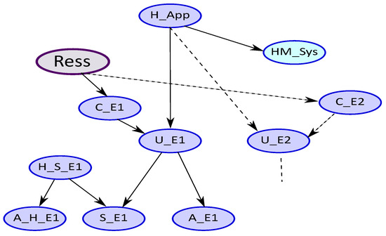
Figure 10.
pattern where the hardware resource is represented by the node .
3.2. Design Flow for an Embedded Version of BN Diagnosis
In this section, we give the basic of the dedicated design tool that we propose to friendly implement the BN monitors onto FPGA support. These works are detailed in previous publications [20,21,22]. We resume the main steps and we enlighten the FPGA implementation of these monitors through an example detailed in Section 5.
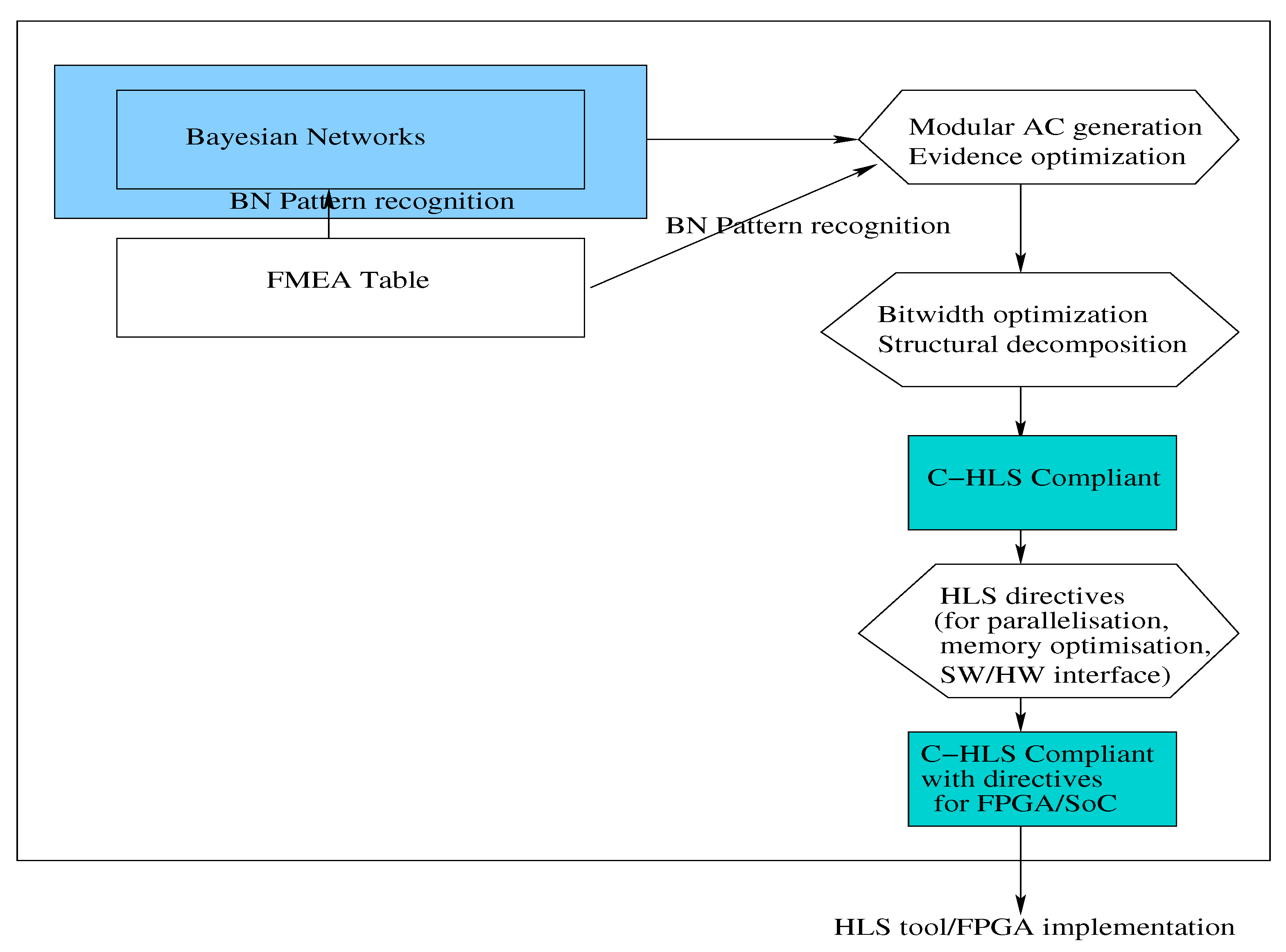
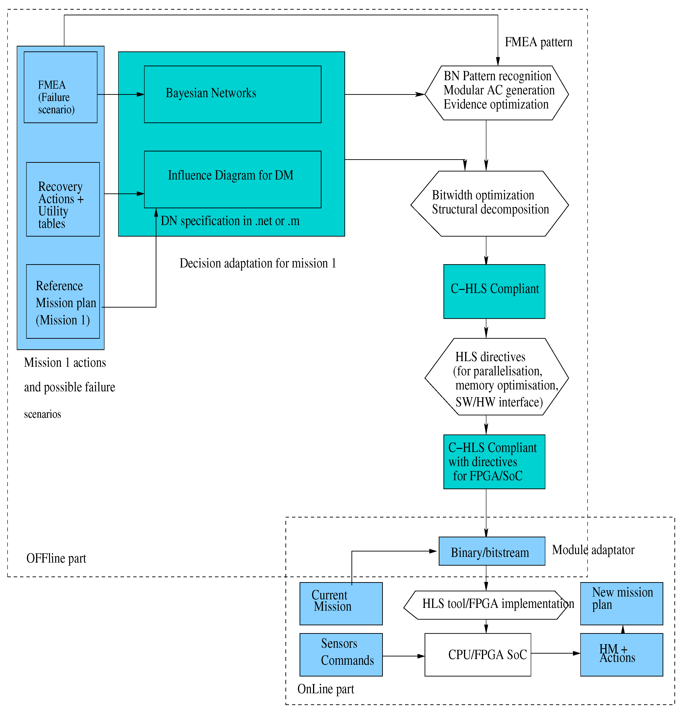
For an efficient implementation of the diagnosis and the mitigation modules specified by Bayesian Networks from FMEA tables, we propose to target FPGA support. The different steps to generate an efficient bitstream are detailed in Figure 11. The main steps are:

Figure 11.
Our design tool proposal for the FPGA implementation of BN monitors from FMEA-like tables (F2F BNTool).
- two kinds of high-level transformations: one dedicated to BN compilation and one more classical related to the structural (or hierarchical) decomposition and to the bitwidth optimization. The first category includes the compilation into an Arithmetic Circuit (AC) form, the evidence optimization. This step provides an C-code (C-HLS Compliant) that can feed HLS tool such as Vivado-HLS from Xilinx.
- HLS directives proposal for the C-code in order to generate efficient implementation onto FPGA (C-HLS Compliant with directives). These directives are proposed to guide the management of the parallelism for the resource usage, the management of the memory and the management of SW/HW interface. These directives are defined in Pragma form using the Vivado-HLS tool [23].
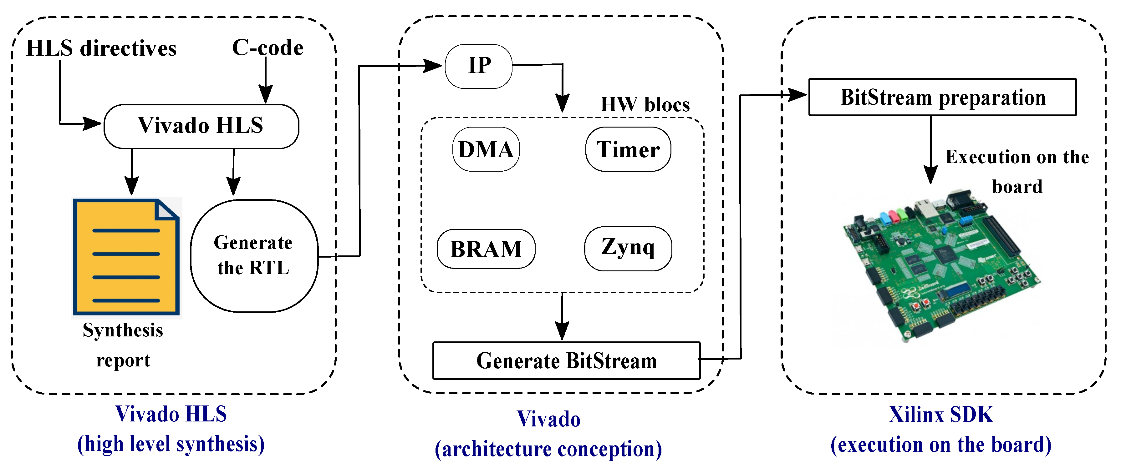
- Integration to HLS tool such as Vivado-HLS whose flow towards a FPGA-SoC board is illustrated in Figure 12. From the implementation on an hybrid FPGA-SoC, different types of interfaces can be used to import the evidence values from the sensors or the parameters of the BN (DMA interface or BRAM interface) via (see Figure 24).
 Figure 12. Integration of our proposal to Xilinx Design flow: HLS directive adaptation, C-code generated by our tool proposal, adaptation with the architecture option (BRAM, DMA).
As inputs, we propose to describe the BN monitors by means of FMEA-like tables associated to three main patterns described in Section 2. These tables can vary in terms of types of error and in terms of error mitigation proposals. From these tables, we generate the BN structures according to the pattern used in the table. After generating the BN model of the monitors, we propose an Arithmetic Circuit (AC) description that can translate the inference computation of BN structures into trees including arithmetics operators (* and +). This AC description can also be directly generated from the BN pattern of the tables. The AC description is an internal form that can be optimized by propagating some evidences associated to sensor activities. Then we can map the code to specific libraries by proceeding to a structural decomposition. Other optimizations like bitwidth optimization can be applied to save resource and to improve performance and reduce energy consumption. This optimization tunes a floating point value to a fixed point one with a limited precision according to an acceptable accuracy. More details on this tuning are given in [22]. The result of the first group of transformations generate a C-description that is HLS compliant. From that point, we feed HLS tool with the C-description. In addition to the one, we can propose some appropriate HLS directives for the parallelism and memory management to provide a better FPGA implementation. Then the HLS tool (Vivado-HLS) is able to provide the embedded version onto the FPGA support. We place our proposal as a front end of commercial HLS tool by proposing the adequate parameters for the HLS directives, the C-code of the BN monitors, as well the adequate interface between the FPGA and the CPU with BRAM or DMA option. The adaptation with the HLS tool from Xilinx is shown in Figure 12.
3.3. Dedicated Optimizations for an Efficient Implementation of BN
We propose to focus on the high-level transformations dedicated to the BN transformations: AC compilation and Evidence optimization.
3.3.1. AC Compilation
BN inference algorithms are used to answer queries when computing posterior probabilities. Classical inference algorithms are based on propagation on the junction tree. A major problem for embedded systems is the complexity of the computation. Algorithms based on ACs are powerful and can produce predictable real-time performances [18,24].
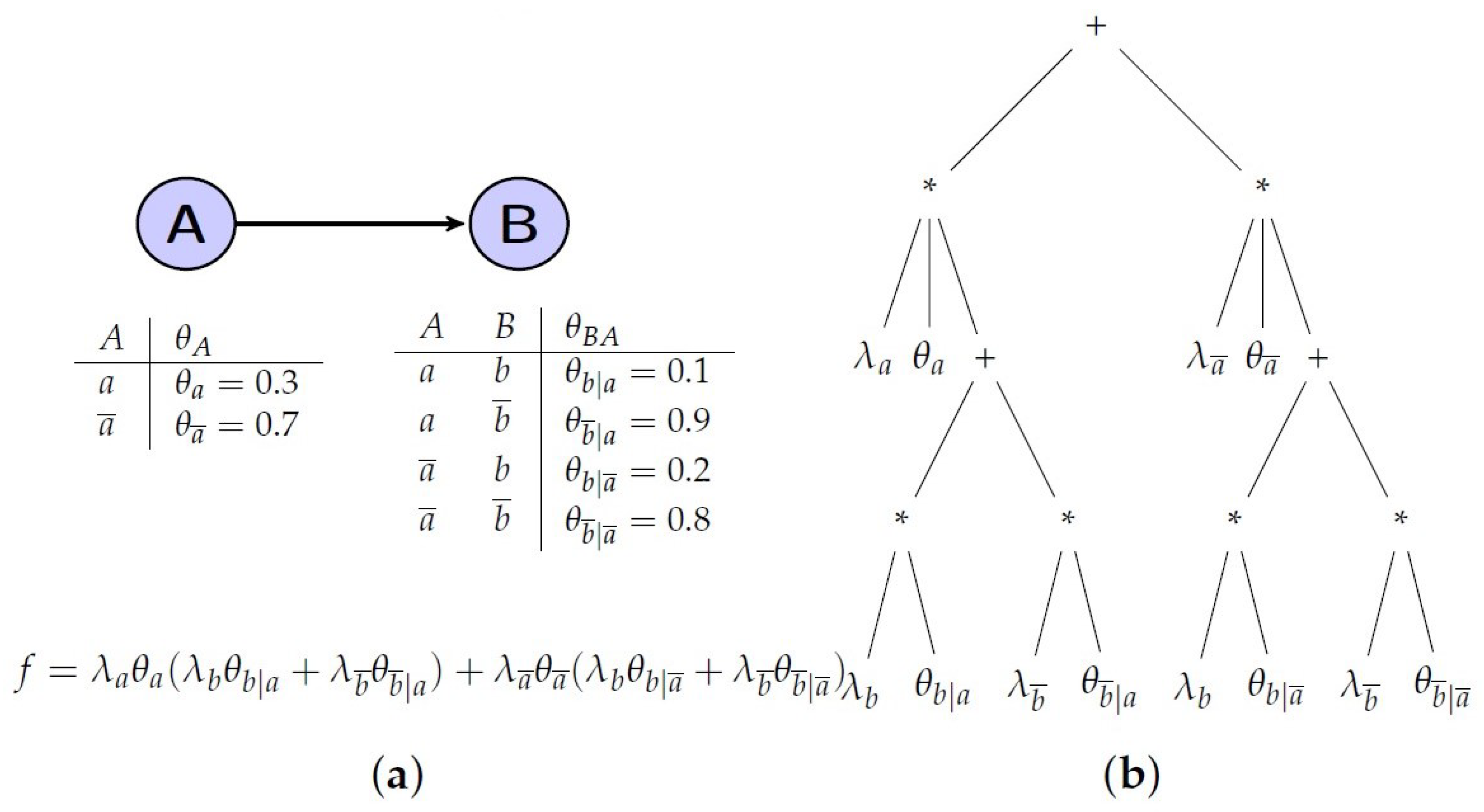
The AC representation of BN can be built from the multilinear function (MLF) f [18] associated with the marginal probabilities of the BN. We show in Figure 13a) an example of MLF to very simple BN structure incorporating two nodes A and B. This MLF can be represented by a tree detailed in Figure 13b). The leaves of the Arithmetic Circuit are (evidence indicator) and (network parameter), and the inner nodes of the tree represent a multiplication (*) or an addition (+), alternately. To compute the posterior probability = (where x is a variable and e the evidence) for the diagnostic, two steps are required: the first to evaluate f(e) and the second to compute the circuit derivatives to obtain f(x,e) = .
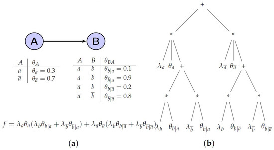
Figure 13.
(a) A simple BN represented by a multilinear function f. (b) The corresponding Arithmetic Circuit of the BN.
The generation of the AC description is based on a new approach of inference computation, which takes advantage of the factorization of the MLF and the regular structure of our general model. The AC MLF factorization is based on the relationship between child and parent nodes. The sub-MLFs for children (if no conditional dependence between them) are represented by a “+” in the AC, and parents combine them with a “*”. In our model, all error type nodes and all monitor nodes are children of the U node (unobservable status of the system). Since there is no conditional dependence between these nodes, their MLF can be calculated separately and in parallel, similar to sub-BNs of each error type, where the parent node represents the error type and the child nodes are the monitor and appearance context nodes.
The corresponding Algorithm 1 is given as the following for the pattern:
| Algorithm 1 to C-code |
| Require: Evidence indicators and Network parameters for each s state of the node U do Compute SubAC for all states () end for Multiply all by network parameters of U node related to s (1) for each s state of the U node do Compute SubAC for system monitor () with the new parameters obtained by (1) end for Compute the probability of the system Health node Ensure: Health probability of the system |
In this algorithm, SubAC represents the MLF with evidences (e) of the sub-BNs associated to the different error types. In addition, the probability of the system Health node is given by Equation (3).
is given for nodes including 2 states (state and state ). If we have several states, we can easily extend the computation of the probability by taking each state into account.
3.3.2. Evidence Optimization
The evidence optimization can be applied to AC structure to reduce its complexity. This transformation propagates constant values for its reduction. These constant values are related to the observability of the BN nodes. In an AC, we can see that the values of evidence of a variable X are equal to:
- when there is no observation on the variable X,
- when the evidence is on the variable X and the observation is x,
- when the evidence is on the variable X and the observation is .
Furthermore, in our examples in Section 2, two types of nodes (observable and unobservable) are known: depending on the type of the BN structure (from FMEA_HM, FMEA_MIT, FMEA_EMB pattern) A, S, C and nodes are observable (evidence), so they take the values or for evidence. The other nodes are unobservable, so they take the values (1,1) for evidence. These observations and the symmetrical structure of the AC make it possible to reduce the AC as follows:
- Delete the left (or right) topmost branch containing a C (or an H) node, and in all sub-branches where C (or H) appears, replace the probability parameters by a choice between the right or left value. We can simplify here, because the value of of these nodes is never equal to 1 at the same time,
- Repeat this procedure for all C and H nodes,
- Fix all the values for the unobservable nodes at .
4. Methodology for the BN Integration at the Mission Manager Level
In this section, we consider the decision-making engine and we propose to incorporate the BN monitors at this level. We focus here on two decision-making models that deal with uncertainty. The first one is a well-known extension of the BN, named Decision Networks [9]. The second model is the Markov Decision Process model that is a very common model [25] used in robotics. The MDP model can be useful to specify to more complex missing. Solving an MDP means choosing the optimal control actions that will maximize a reward or, equivalently, minimize a cost criterion. Several cost criteria are classically used. Typical reward (or costs) criteria include instantaneous or average discounted and undiscounted costs over finite or infinite time horizons in continuous or discrete time. In our setup, we are concerned by the undiscounted cost on finite horizon in discrete time.
For the both models, we show how they can cooperate with the BN monitors to elaborate a context-aware decision making including some safety requirements. These models can be used for a high level model for mission management of autonomous vehicles. We show how we can specify the mission planning in a case of UAV with DN and MDP models. Finally, the implementation of the decision-making models on FPGA-SoC platform is proposed with a dedicated design process.
4.1. Decision Networks (DN)
DN are directed acyclic graphs (DAG) with nodes belonging to three different categories: chance nodes (ellipses or circles in graphical notation) represent (as in BN) discrete random variables; decision nodes (rectangles) represent actions or decisions with a predefined set of states; value nodes (diamonds) represent utility (or cost) measures associated with random or decision variables. Edges represent direct (possibly causal) influence between connected objects. An example of DN (cf. Figure 14), linking the two BNs and the possible actions to activate by a utility table. The table (detailed in Table 4) gives a score for each action relative to the BNs, and the choice of the adequate action is given by computing a utility function () for each action.
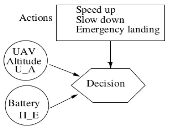
Figure 14.
Decision Network (DN) example to make a decision between the different actions to choose (Speed UP, Slow Down, Emergency Landing) taking into account the state of the unmanned aerial vehicle (UAV) in altitude and the health status of the battery.

Table 4.
Utility table for decision making with DN associated with the actions Speed Up (SU), Slow Down (SD) and Emergency Landing (EL).
To compute the utility function, we need the probability of the UAV state and the battery state representing the correct functioning. These latter ones are provided by BN. The utility function of each action is equal to the sum of the products of the action with the adequate probability concerning the UAV state and the battery state. The action to be chosen is the action that has the highest utility function.
Let us consider the example of Figure 14:
: the highest utility function where each utility function is equal to
which represents the sum of the products of utility values from the Table 4 with the adequate probability concerning the UAV state () and the battery () from Figure 14.
In this example, if we take the BN probabilities , and the utility table of Table 4, then , and which means that the action chosen is (“Speed up”) this case.
4.1.1. Mission Planning Description with DN
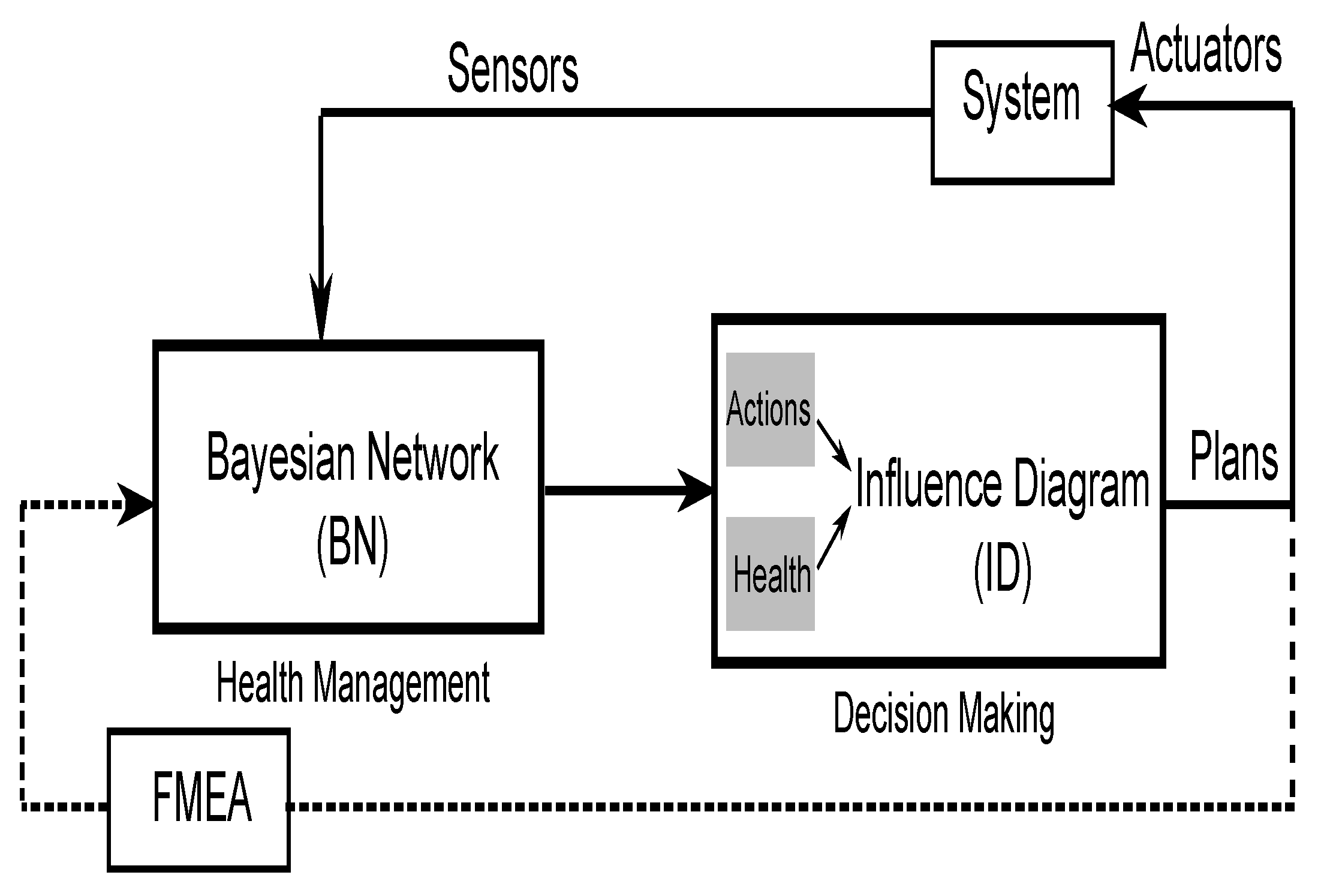
Figure 15 illustrates our approach in a case of a mission for an autonomous vehicle, where we combine a Health Management modules with a decision-making module. The first module is based on Bayesian Networks and has been developed from FMEA tables. According to the reference mission, the module allows, from information given by sensors, to continually monitoring the system, to check the mission reliability and to be able to detect and locate a failure with BN monitors. The decision-making module is a Decision Network (defining the Influence Diagram), taking a list of possible actions and the results of the Health Management modules and gives the adequate recovery action to define the new mission plan.

Figure 15.
Embedded Decision Network for an autonomous vehicle.
4.1.2. The DN Design Tool for an Embedded Implementation
To design dedicated Decision Networks incorporating diagnosis or mitigation, we can extend the BN design tool as shown in Figure 16. In this version, we have the three main layers:
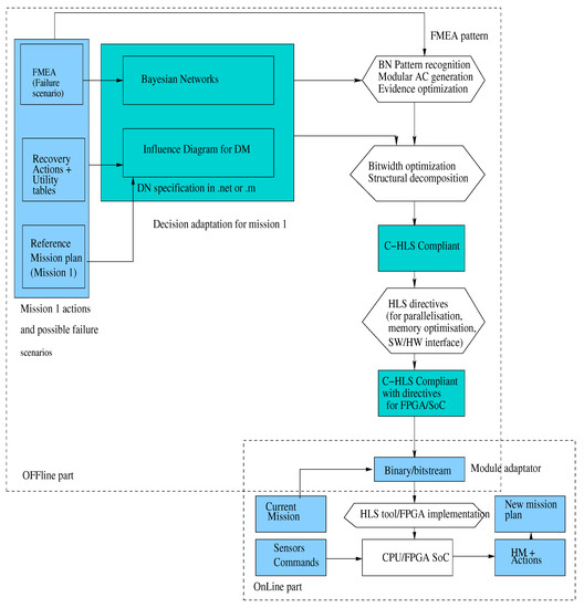
Figure 16.
HLS design tool proposal for Decision Networks onto FPGA SoC support.
- In the first layer, a friendly front-end interface to generate the Bayesian Network model from FMEA-like analysis and incorporate to decision process for a DN definition. The DN specifications can be expressed in format or format in order to be compatible with other tools such as Genie [26], BNT [27] tool for Matlab.
- In the second layer, the Bayesian core tool takes a DN as input. First a series of dedicated high-level transformations are proposed for the BN part: AC compilation based on model patterns, evidence optimization. Then optimizations on the whole DN part are proposed such as bitwidth optimization and a functional/structural decomposition based on the choice of the elementary function for a hierarchical decomposition before the generation of the C-code.
- In the second layer, a refinement of C-code is proposed by introduction of HLS directives for code parallelization, memory and interface management. This latter C-HLS compliant code is tailored for a complete FPGA implementation on ZedBoard.
The second layer proposes high-level transformations and provides parallel opportunities for the code independent of the target platform. These high-level transformations are mainly detailed in Section 3.2. The third layer gives an more practical guide for a parallel implementation on a SoC/FPGA platform. This latter one is platform dependent.
4.2. Markov Decision process (MDP)
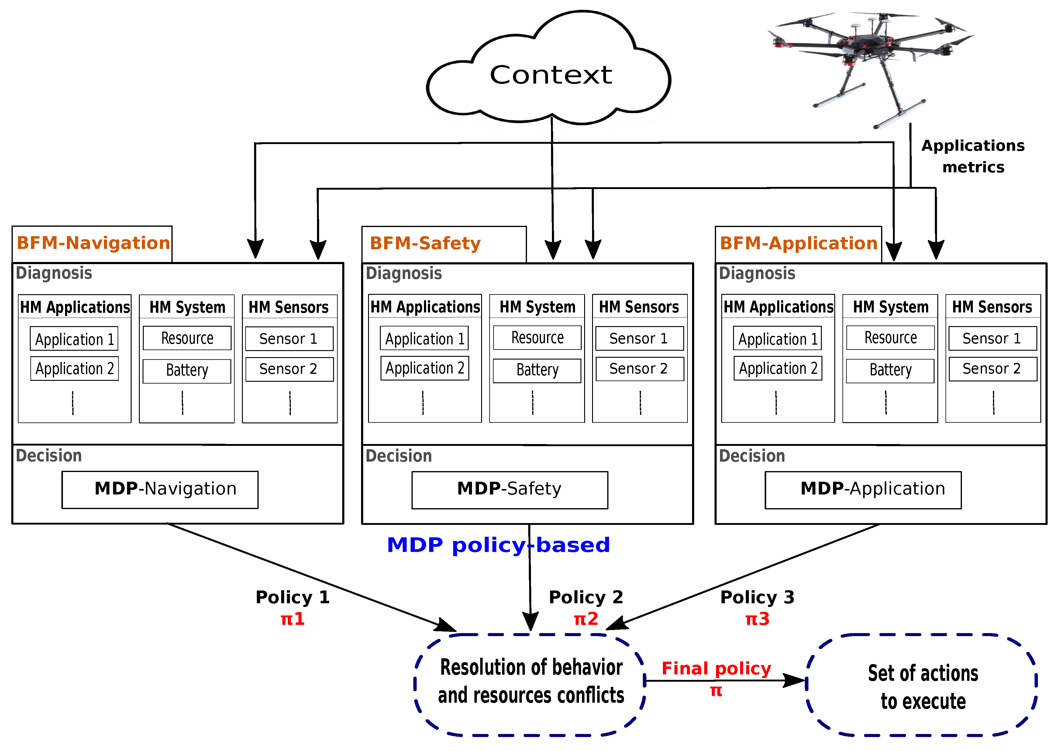
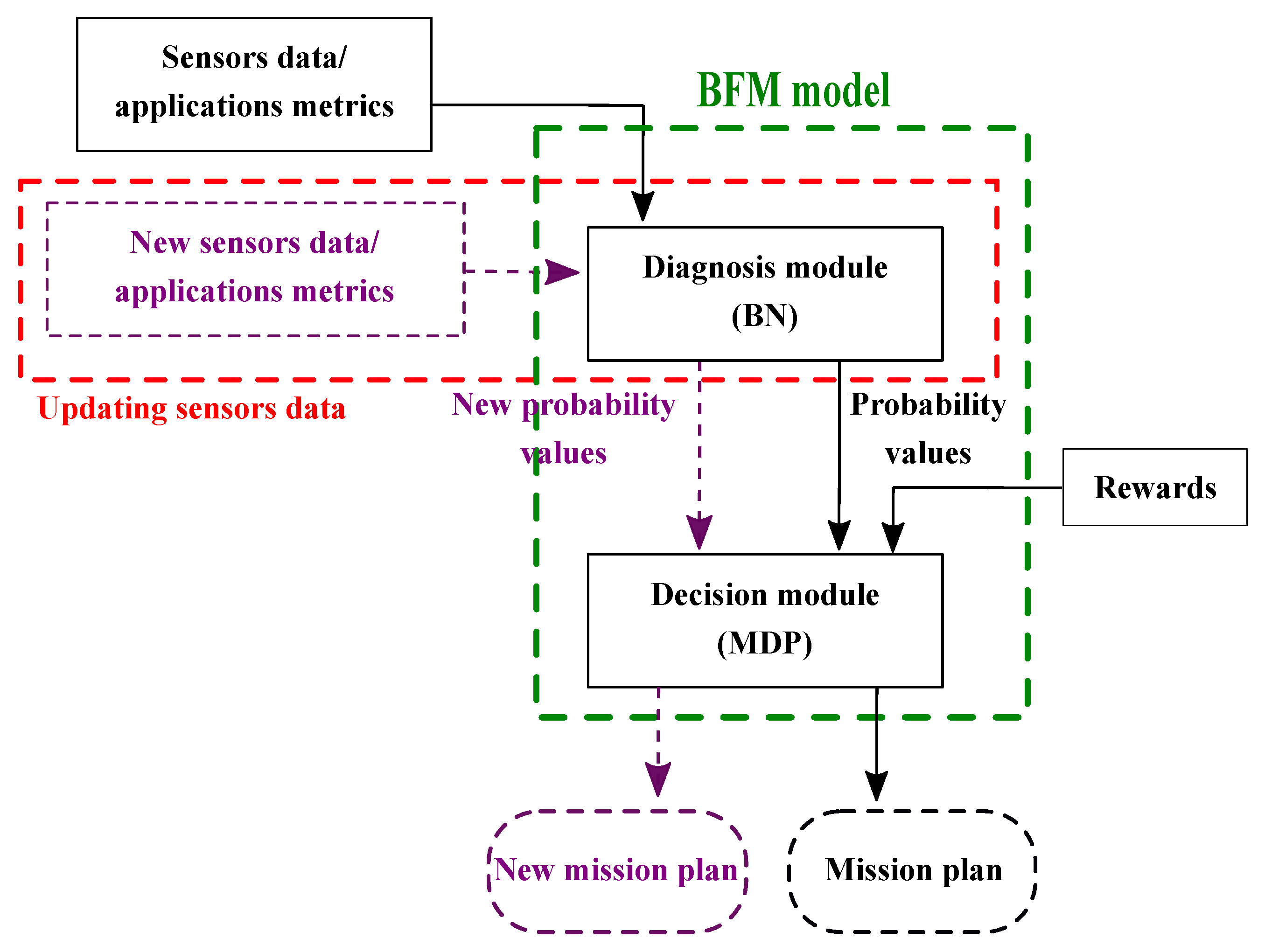
In this section, we propose to integrate BN to Markov Decision Process (MDP) [28] to elaborate a more complex mission planning. This model is named BFM cmodel (Bayesian network built from FMEA table to feed the MDP model) [29]. The BFM model relies on an architecture based on two principal modules: the diagnosis module based on BN and the decision-making module based on MDP. Figure 17 shows the proposed architecture where the diagnosis modules are organized in three categories: health of the sensors, health of embedded applications in term of QoS and the health of the system (computing resources, battery, etc.). The decision modules manage the mission and are specified by the mission designer using the MDP model.
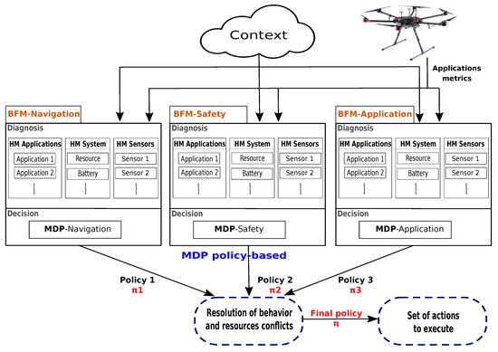
Figure 17.
Concurrent MDPs for the mission-planning.
The diagnosis module computes the probability of the health status of the different HW/SW components of the system (sensors, applications, etc.) considering the context hazards and the internal event for the components. Therefore, different types of Health Management (HM) are available to feed the decision module by probabilities (applications HM, sensors HM and system HM). The “applications HM” contains multiples HMs, one for each application that can run on the embedded system (e.g., tracking, navigation, obstacle avoidance, etc.). The “sensor HM” also contains different HMs for the different sensor or set of sensors (e.g., GPS, camera, etc.). Finally, the “system HM” includes the HM of the other components of the system as resources (i.e., CPU load, etc.), battery, etc. For the HM generation, we can use the different patterns ( pattern, the pattern and the pattern) introduced in Section 3.
The decision module uses the MDP to specify the mission and to select the set of actions to execute. The MDP model takes as inputs the probabilities provided by the different HM of diagnosis module. These probabilities are carried by the transition functions of the MDP model. The MDPs consider the potential sensor failures (sensor HM), system failure (resource HM) and the different alternatives for the embedded applications (application HM).
The mission can be expressed using concurrent BFMs. The different BFMs highlight some functionalities (or missions phases) of the mission. For instance, we can have three main functionalities:
- Navigation functionality (BFM navigation): considers all the applications needed to achieve navigation phase. These applications are for example take-off, path planning, obstacle avoidance, etc.
- Safety functionality (BFM safety): consists of a set of application that used for mission and autonomous system safety. These applications are landing, obstacle detection and avoidance, emergency search landing area, etc.
- Application functionality (BFM application): consists of a set of applications using to achieve the mission aim like target detection, tracking, indoor/outdoor mapping, etc.
For an autonomous system, we need an embedded mission planning. The diagnosis part continuously monitors by the help of the sensors or by the help of internal flags the embedded system and the environmental context of the mission. This part is fed by the sensor data or by the application metrics. Then as shown in Figure 18, the decision module can update its decision online taking the new probabilities of the diagnosis into account in order to generate a new mission plan.
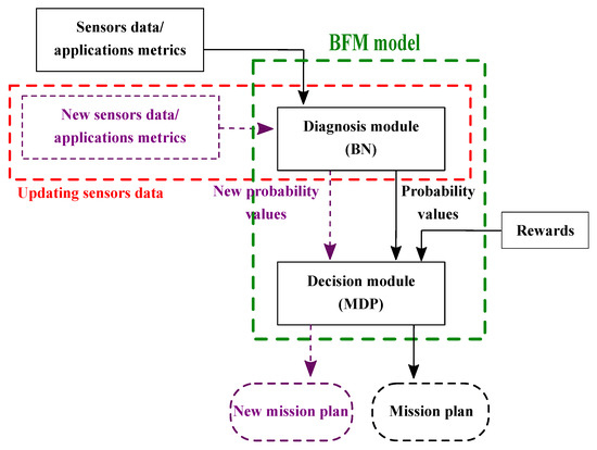
Figure 18.
The execution of the embedded BFM model.
Example of Mission Planning with BFM Model
We take as a case study a tracking mission where the aim is to detect and track a potential target (for more details see [30]). We define the mission planning using the concurrent BFMs (BFM navigation, BFM landing, BFM tracking). Each BFM is associated to a MDP detailed as follows:
- For the BFM-navigation: the MDP of the navigation phase includes 9 states (ex: waypoints states, obstacle detection state, etc.) and 7 actions (example: take-off, obstacle detection, follow trajectory, etc.) which involves 7 transition matrices of size 9 × 9 and a rewards matrix of size 9 × 7.
- For the BFM-landing: the MDP contains 10 states (landing state, found landing area state, etc.) and 6 actions (search landing area, landing, etc.). This gives 6 transition matrices of size 10 × 10 and a rewards matrix of size 10 × 6 generated for the landing phase.
- For the BFM-tracking: the MDP contains 12 states (target detection state, tracking states, etc.) and 10 actions (target detection, tracking, stabilization, etc.). Thus, its gives 10 transitions matrices of 12 × 12 size and a rewards matrix of size 12 × 10.
In Section 6, we propose a hardware and software implementation of the MDP part of the BFM model to show the extra-execution time and speed up gain, concerning the pure decision-making modules without the diagnosis extension. The implementation of the HM modules associated to the BN part of the BFM has been explained and already explored in Section 3.2.
5. Study Cases
In this section, we present first different study cases that illustrate the different types of BN monitors: a sensor monitor with the GPS and an application monitor with the tracking application. Then we explore some HW implementations of scalable monitors using the design flow detailed in Section 3.2. Finally, we present the result of the HW exploration of a complete DN decision-making engine.
5.1. BN Generation Examples
We illustrate in this section the use of the pattern driven approach for two cases of study. For more details about these examples, please refer to [30,31].
5.1.1. Example 1 Sensors Monitoring: GPS Example
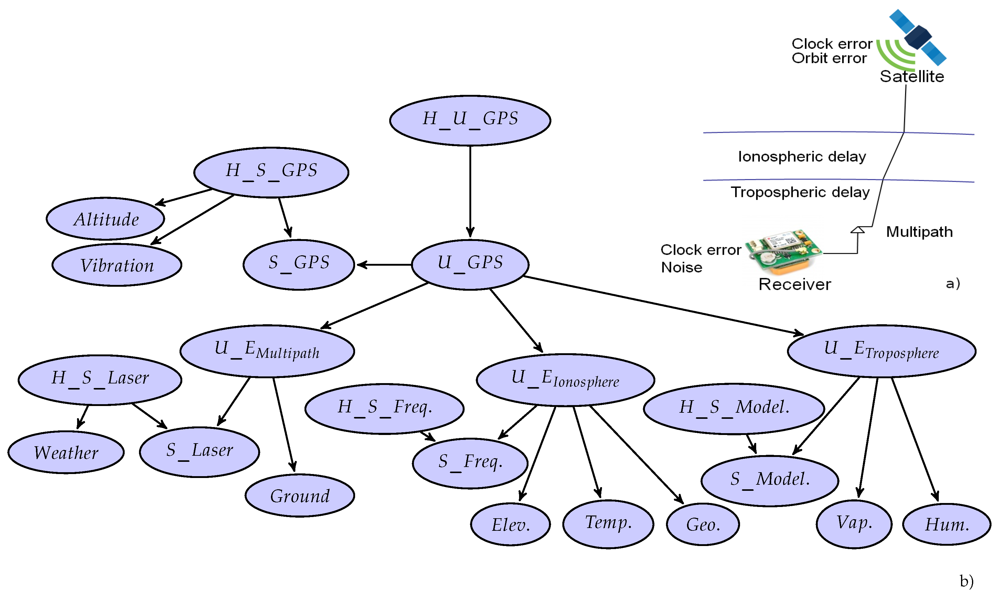
A GPS receiver is used worldwide and offers a very affordable solution with limited on-board processing, in contrast to vision-based approaches. Nevertheless, the GPS system is error-prone. The accuracy and the reliability of the position given by a GPS depend on contextual factors affecting the satellite signal during its propagation or its reception. The sources of error can be identified at the system level by means of additional bias for the computation of pseudorange measurements [32,33]. These measurements can tune the GPS positioning accuracy from slightly imprecise to completely faulty. They can be improved by introducing observations [34] or real environments [35]. The aim of the HM for GPS is to estimate the positioning deviation in terms of probabilistic values considering the context of use on the basis of sensor information. The HM of GPS can be modeled by means of BNs from the FMEA. The main GPS localization errors are shown in Figure 19a and the corresponding FMEA is represented in Table 5.
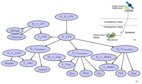
Figure 19.
(a) Illustration of the different types of error for the GPS receiver. (b) The BN monitor generated from the FMEA-like table of Table 5.

Table 5.
FMEA for GPS.
The BN for GPS HM is given in Figure 19b. We can obtain the BNs from the FMEA of the GPS (Table 5) using the proposed model. The GPS localization system accuracy is mainly evaluated by the 4 error types, which themselves are monitored by software or hardware sensors as well as their appearance contexts. The sensors themselves can be faulty and their Healths are reinforced by the appearance contexts. An example for laser sensors is the weather node, which can be given by weather forecast or temperature sensors.
5.1.2. Example 2 Application Monitoring with Mitigation: Tracking Application Example
The FMEA table contains the possible errors that can decrease the QoS of the tracking application considering the context. Depending on environment factors, different parameters or versions of the tracking algorithm can be considered to achieve a good QoS, as shown in Table 6.

Table 6.
Failure mode effects analysis applied to the tracking application.
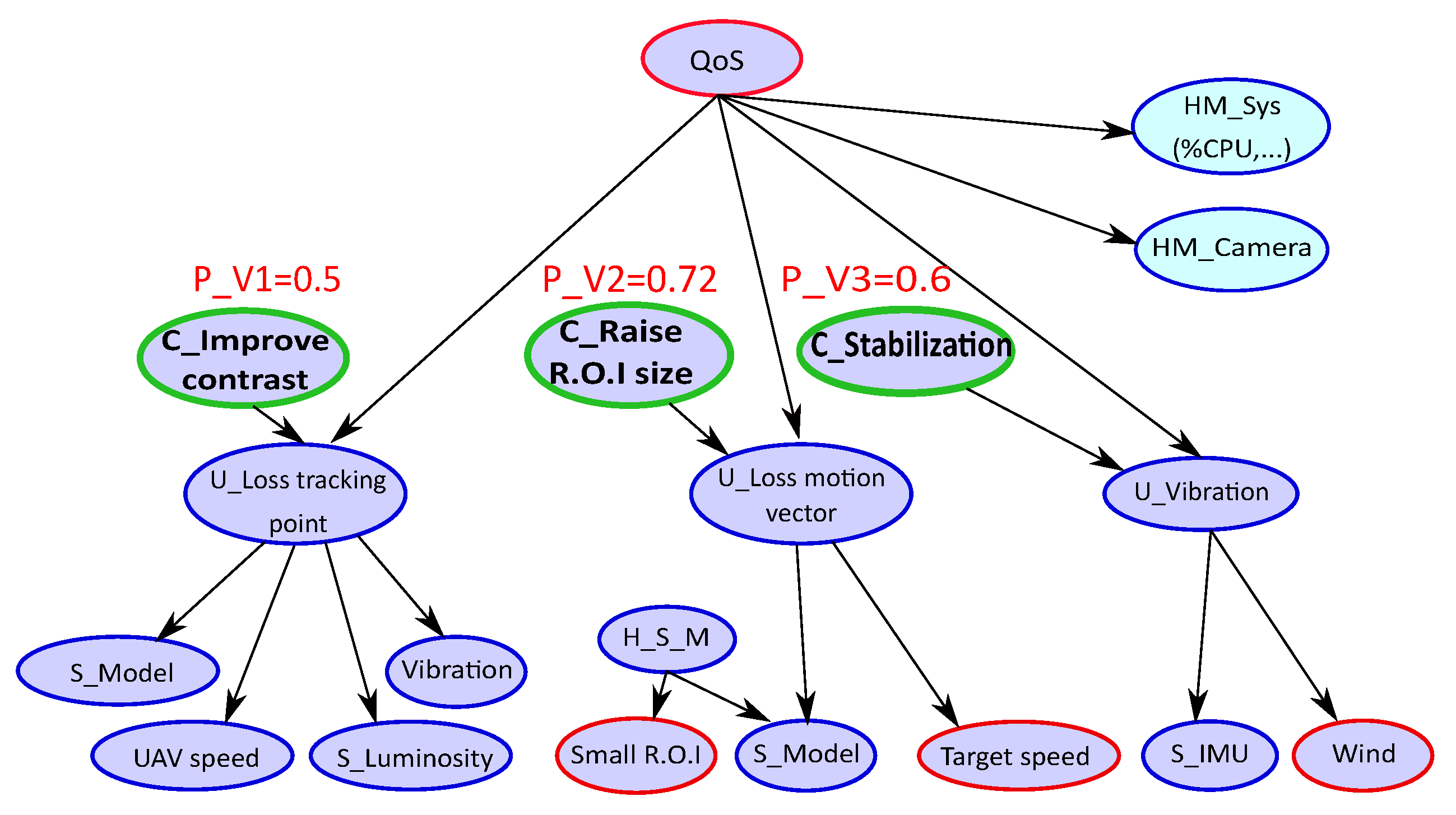
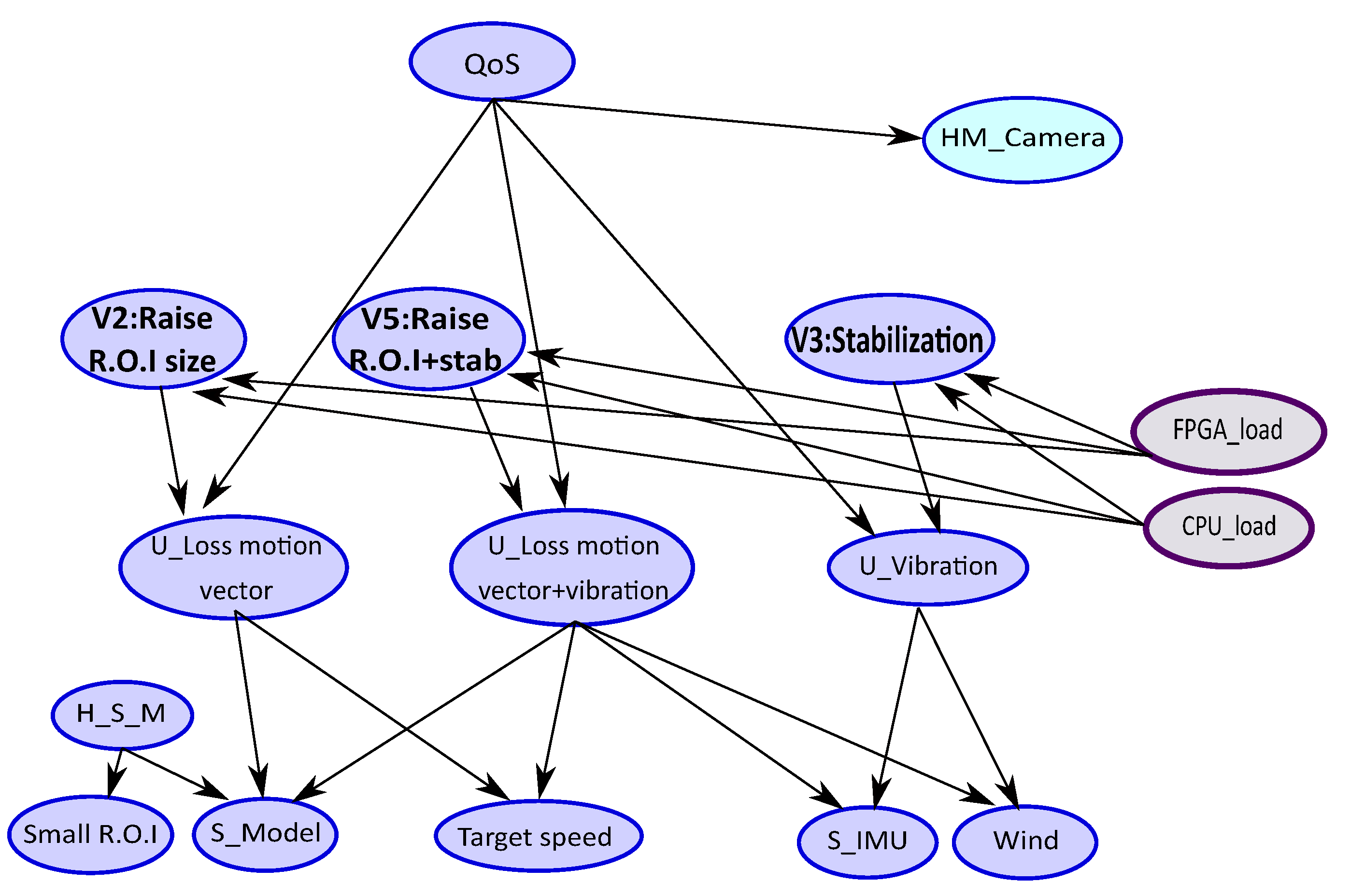
Figure 20 shows the translation of the FMEA Table 6 of the tracking application into a BN model. The root node represents the QoS of the tracking application to maintain when an error context occurs. The U_nodes indicate the unobservable state of the errors of vibrations (U_Vibration), motion vector (U_Loss motion vector) and error of point tracking (U_Loss point tracking). These types of errors are monitored by physical (sensors) or software measurements denoted by S_nodes as (S_IMU, S_Model, …) and appearances context. Monitor nodes can also have a health status indicated by the H_S_node as (H_S_M) in a certain appearances context A_H_nodes (e.g., Small R.O.I). The C_nodes represent the solution proposals that can mitigate the observed type error (e.g., C_Stabilization in the case of vibrations error), and ensure to maintain the expected application QoS level.
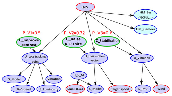
Figure 20.
BN for tracking application with mitigation proposals.
The mitigation capability of the BN is shown in Figure 20. The probabilities associated to the mitigation nodes (green nodes) are computed with the expected value of equal to high. As mentioned previously, the nodes represent random variables. Each node has two states except the QoS node which has 3 states (high, medium, low).
In this example, we observe a context with wind and target speed and we fix the probability (evidence) of QoS to be in the state “high”. The wind introduces some vibrations and tracking error occurs. The target speedup can also lead to a wrong motion vector estimation if the R.O.I is too small regarding the target speed. These observations are reported in the BN by providing evidences on these context nodes, represented by the red nodes in Figure 20. We obtain a probability of 60% to activate the stabilization and 72% to activate new tracking version by increasing the window (R.O.I) size. In this example, the efficient solution is to increase the R.O.I size.
5.1.3. Example 3 Resource-Aware Monitoring for the Tracking Application
The performance of an application depends on its implementation. For instance to be able to achieve 150 frames per second (FPS) for the tracking application, we need a parallel version implemented with FPGA hardware resources. For each embedded application, different variants can be defined to fit the performance needs. For the tracking application, we can have for instance a fast version (version A) of 150 FPS that runs on FPGA using all resources, a slow one (version C at 5 FPS) that runs on only, and an intermediate one (version B running at 50 FPS) that runs a the with a coprocessor implemented on the FPGA. In this section, we show how we can enrich the to take into account the resource constraints of the system and the performance constraints.
First, the resource constraints are introduced into the as BN nodes. The probabilities of these nodes correspond to the load of the device chosen to execute the embedded applications. A large panel of computing resources can be considered such as GPU, multi-cores FPGA, or heterogeneous architectures such as FPGA-SoC. The resource constraints can be roughly expressed in terms of number of cores for multi-core CPU, number of workgroups for a GPU and in terms of number of tiles (predefined dynamically reconfigurable area) for the FPGA. In a case of hybrid devices like FPGA-SoC (e.g., Altera Cyclone V, Xilinx Zynq), we define the metric corresponding to the resource occupancy for one application , where the fractional part of represents the load and where the whole part of represents the load in terms of tiles.
These two loads ( and ) can be separately modeled with two different nodes in the whose number of states depends on the parallel grain chosen for each support. For instance, in a case of the , the number of states can be associated to the number of tiles; and in a case of , the number of states depends on the different interesting thresholds for the use (typically 20, 40, 60, 80%). Figure 21 illustrates the insertion of this resource constraint into the resource nodes. In this example, we consider a FPGA-SoC device and two resource nodes are inserted. A total of 4 tiles are under consideration for the , and two thresholds (at and at ) for the . The values of these nodes correspond to information monitored by the system and based on this information, we estimate the capability of the chosen version to be executed by the device. We estimate two possible states or of the version. This estimation is elaborated through the conditional probability tables of the solution nodes of the related to the resources nodes. If we consider the version A of the tracking, we need to use all the resources of the FPGA, so the activation of this version is possible only if the monitor of system indicates a total availability of the FPGA.
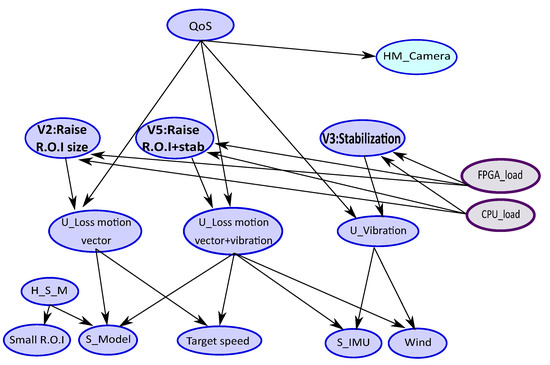
Figure 21.
Resource-aware Health Management (HM).
5.2. Experiment on FPGA-SoC Based on FMEA_HM Pattern
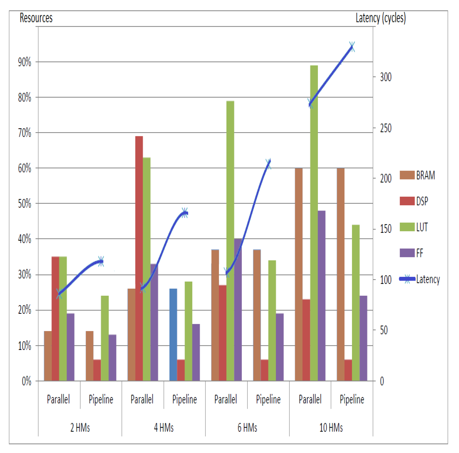
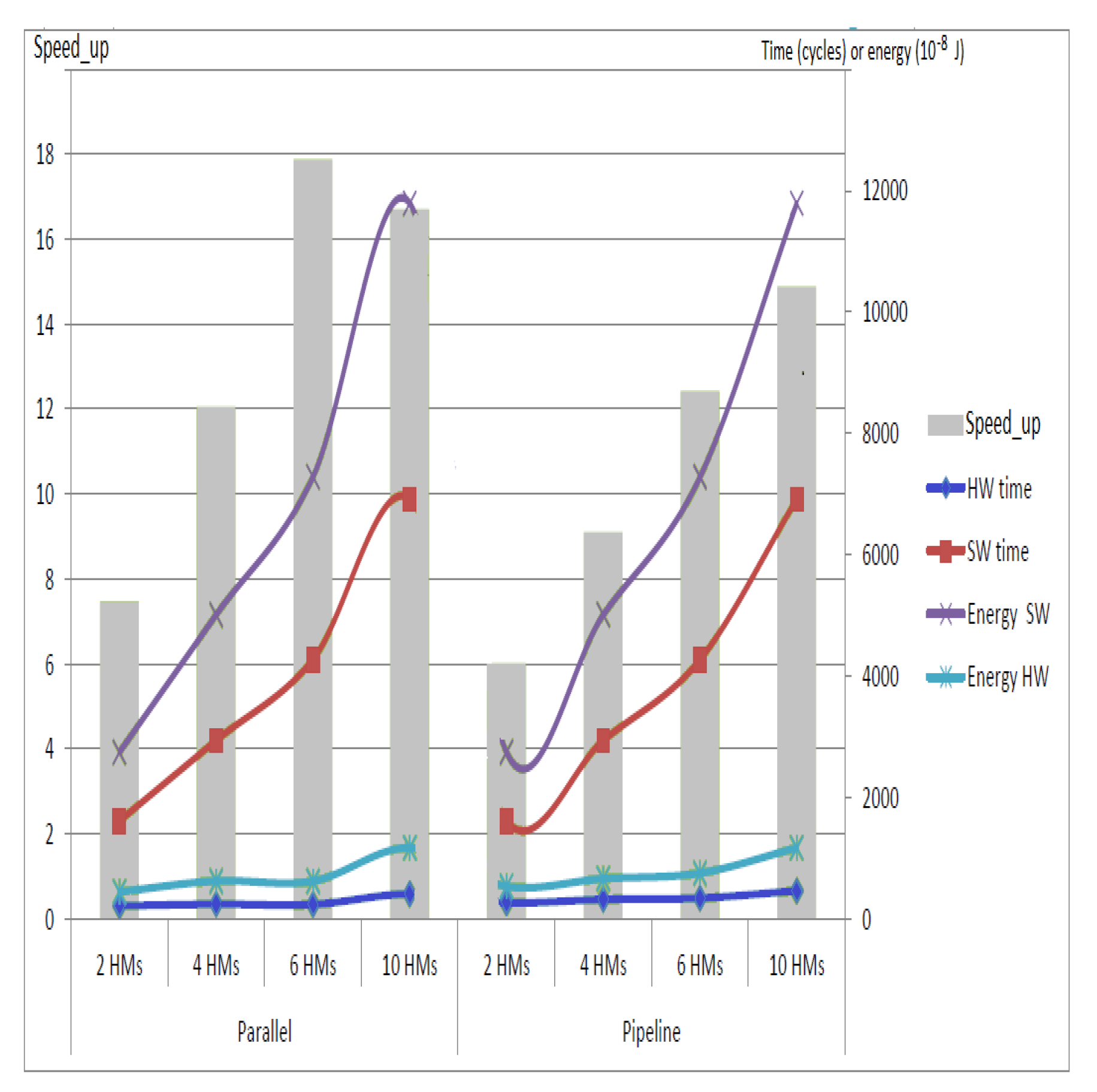
To give an idea of potential interest of an FPGA implementation of the BN diagnosis, we propose to explore different implementations of different variants of HM using the pattern. We take a basic HM incorporating 3 error types and we vary the number of HM varies from 2 HMs to 10 HMs. The complexity of an HM with 3 error types corresponds to BN with 27 nodes. The number of nodes of each HM corresponds to the BN generated with the pattern with 3 error types and two appearance contexts for each error type and two appearance contexts for each sensor that monitors the error type. Then the complexity of one HM is equal to 27 nodes. The implementation of 10 HMs has a complexity of 270 nodes. The Figure 22 and Figure 23 summarize the results. For these experiments, we propose two strategies. The first one is that all the HMs are computed separately and in parallel (with resource limitation when necessary), and the second one is that one HM is used for all the computations which are in pipeline.

Figure 22.
Results of the HW implementation for the scalable BN monitors in terms of FPGA resources (BRAM, DSP, LUT, FF) and in terms of performance with pipeline and parallel directives.
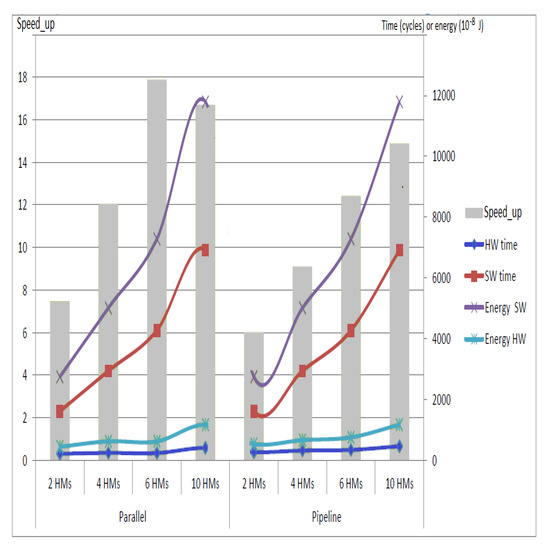
Figure 23.
Comparison of the HW and SW implementations of the scalable BN monitors in terms of latency and energy consumption.
Figure 22 shows the used area and the latency for the different cases, and Figure 23 gives for the same cases the HW and SW runtime, the speed-up and the energy consumption. From Figure 22 we can deduce that the area grows with the number of HMs, in the case of parallel strategy because each HM operates independently and there is no resource sharing. Note that it is necessary to limit the resources in case of 6 and 10 HMs, otherwise it exceeds the capacity of the device (in this case study, we use a Zynq xc7z020 from ZedBoard [37]). In the case of pipeline strategy, the resources used grow slowly, which amounts to use the same resources. In the case of parallel strategy, the latency grows, too, with the number of HMs, which is due to the data reading, but the latency gap between 2 HMs, 4 HMs and 6 HMs is small. However, the 10 HM latency is more important, because of a big limitation of resources. In the case of pipeline strategy, the latency grows, too, with the number of HMs, since the interval of computation grows with the number of HMs.
From Figure 23, we confirm that we can have a good speed-up with the HW implementation. In the case of parallel strategy, we observe that the speed-up is less important for 10 HMs because of the big limitation of resources. The speed-up and the energy consumed are better in the case of parallel strategy due to the interval of computation between two HMs in the pipeline strategy.
These results firstly show the impact on performance, resources and energy consumption of a generic Bayesian network based on FMEA_HM pattern by varying the number of error types. We can conclude that HW accelerations and resources increase with the number of error types, because each type of error represents an independent Bayesian subnet. We achieve a speed-up greater than 14 with an FPGA implementation for 10 HM (270 nodes) and with a very low energy cost. The strategy to adopt (parallel or pipeline strategy) for generating an efficient HW implementation onto FPGA depends on the complexity of the BN monitors and on the resource capacity. In a general case, the parallel strategy offers better speed-up but the needs of resource is bigger. Depending on the resource capacity and on the timing constraint, pipeline strategy can offer a good trade-off.
We see in this example that BN monitors are good candidate for HW implementations. We obtain a significative speed-up comparing to the SW version. This means that we can easily consider these HW implementations for an embedded version of autonomous vehicle. In the next section, we study how to incorporate them into a decision-making mechanism of the mission manager.
5.3. HW Exploration for DN
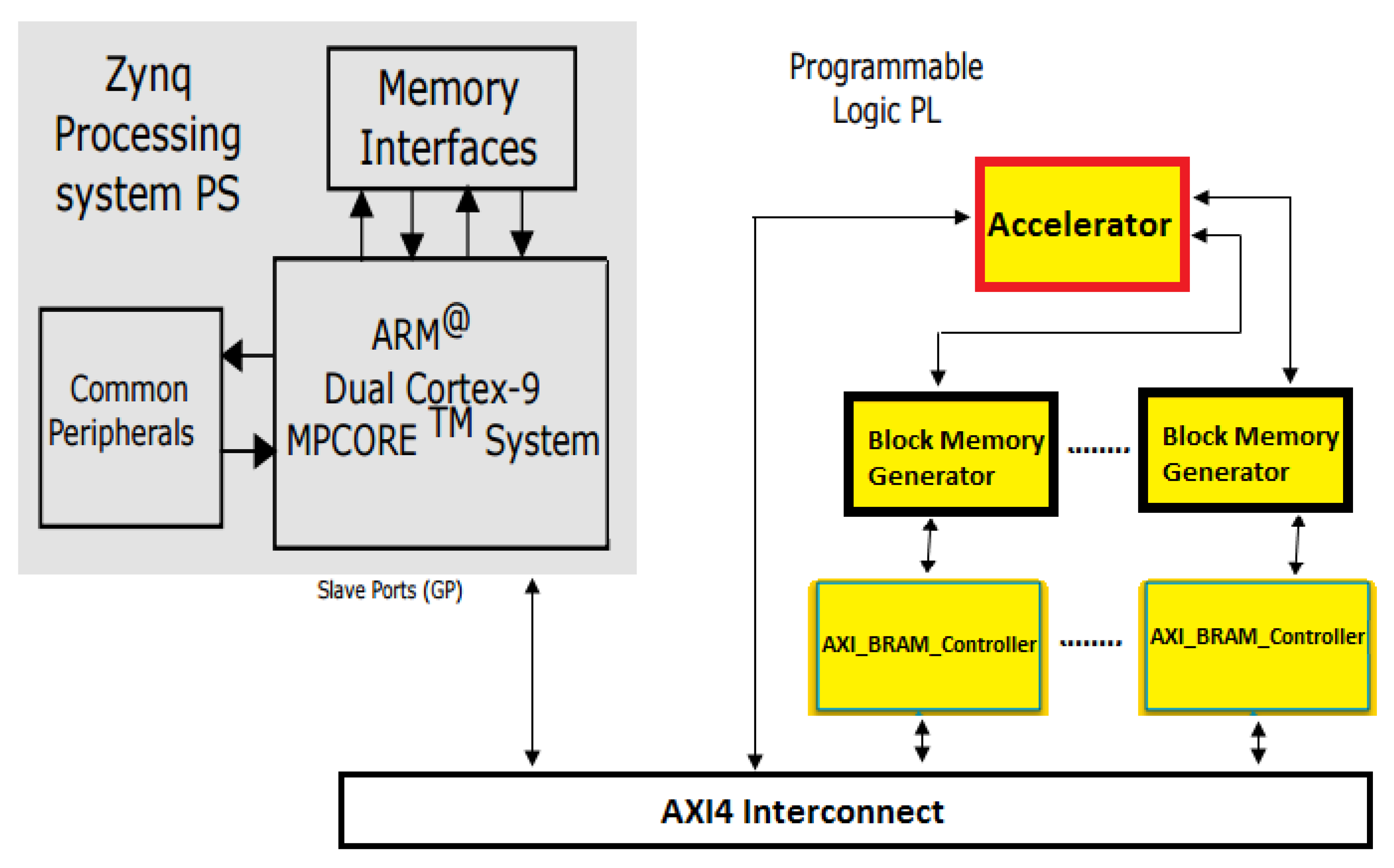
In this part, we propose to explore a co-design implementation of the decision-making modules. To achieve a co-design implementation, we propose to target a ZedBoard incorporating a hybrid Zynq processor with processing system and programmable logic on chip. We couple our design tool to the commercial tool from Xilinx (Vivado-HLS, Vivado and SDK) such as in Figure 12 to target the Zynq processor. As shown in Figure 24, the target architecture is built around the ARM Cortex-A9 processor (Zynq processing system PS; the SW part). The processor is communicating with dedicated HW accelerators (from the Programmable logic part) using the programmable logic through an Advanced eXtensible Interface (AXI) bus.

Figure 24.
Architecture of Zynq processor and BRAM interface.
We consider for the co-design implementation on the Zynq processor, the BRAM architecture for the communication between the HW and the SW parts (see [20] for more details). For Bayesian networks based on FMEA, we propose an architecture where the parameters of the BN are stored in BRAM and can be modified using an Controller, which manages the data transfer between the BRAM blocks and the DDR memory. This architecture allows fast data transmission. Note that the probability tables can be sent when they are fixed and can be modified on-line via the controller. In practice, the update rate is low and the probability tables can often be considered static during a mission. The evidence indicators (Boolean values) are provided by the sensors and are updated for each computation according to the sensor frequency. To minimize time and optimize resources, they are concatenated by 32 and sent via Controller. The health status or decision results are sent via an AXI lite bus. If many results must be sent, we can also use a BRAM for output. Figure 24 represents this architecture for the HW/SW experiment implementations on a ZedBoard.
We propose here the study of the decision with the DN model by varying both the number of Bayesian networks and the number of actions. We explore here a co-design approach for the DN model by varying the number of actions and the number of BNs. Table 7 summarizes the results of the decision making using the pipeline strategy for BN with average data partitioning and all BN with 3 error types. For this experiment, we propose two types of implementation for the DN: a complete one in HW and a mixed one (BN of the DN in HW and the pure decision-making part od the DN in SW).

Table 7.
Resource and performance of the DN implementation by varying the number of Bayesian networks and actions.
We can see that in all cases the implementation of the whole DN in HW is more efficient, with a good acceleration. When the number of BN is small, a mixed implementation may be possible when the number of actions is also small. We can also see that the HW time evolves linearly in number of actions and exponentially in number of Bayesian networks, which is due to the size of the utility table which is exponential in number of Bayesian networks and of the multiplications of all the values of this table by the probabilities of BN in the calculation of the utility function. The resources also increase with the number of BN and actions, which can be explained by the parallelism in the calculation of the utility functions of the different actions, as well as the products of multiplications of the BN probability and the utility table.
Then, we can conclude that a complete HW implementation is the most efficient but can use a lot of resources. The mixed implementation (state of health in HW and Decision in SW) is interesting when the number of actions is small. The choice of concerning implementation of DN is mostly made according to the need for performance/energy consumption and available resources. For practical case, the mixed solutions are most of the time enough for the decision process of the mission manager.
6. Discussion
We propose in this section a discussion onto two aspects concerning the BN monitors. The first one is the issue of the BN parameters and the second one is about their incorporation into the embedded decision-making engine at mission management level.
6.1. BN Parameter Issue
One of the problems when dealing with a Bayesian Network (BN) is to define its parameters (the probability tables). Generally, these probabilities are defined by an expert of the system. However, this expertise may be incomplete or impossible to achieve in some domains and/or systems. In this case, it is necessary to use a learning method for the BN parameters [12]. There are different learning methods for BN parameters in the context of complete data [13] or incomplete data [14]. In the real application like the evaluation of autonomous system health status, the expert databases are often incomplete. The missing data can be provided by sensor failures, inaccurate measurements of sensors data, etc. In this case, it is possible to learn the BN parameters from the databases using the Expectation and Maximization (EM) algorithm [38]. As this algorithm can consider the structure of the BN, the learning phase can be manageable. In [39], we show that we can reduce the timing in the learning phase if the structure of the BN is known in advance.
6.1.1. Description of EM Algorithm
EM is a classical algorithm used to learn and estimate the parameters (CPT probability) of BN under incomplete observed data. EM is an iterative algorithm that works in two steps step E et step M [40].
- Step E (expectation): estimate the missing values from the current parameters . For each BN node V and for each sample of the incomplete database, we compute the conditional probability P(|) (Equation (5)). The computation of these probabilities is based on the inference process using generally the junction tree algorithm.where indicates the evidence of the whole measured data and pa() = represent the status of the parent node of . is the conditional probability at time t of and its parent knowing the value of the observation about V and . Finally, N represents the sum of the probabilities of all the instances of node .
- Step M (maximization): re-estimate the parameters from the results obtained from step E by applying the maximum likelihood or the maximum a posteriori approaches. The most used approach is the maximum likelihood. Therefore, the probability at the next time step is equal to the occurrence of divided by the sum of all the occurrences of across the whole database (Equation (5)).
The effectiveness of the EM algorithm depends on the rate of missing data in the database. In previous work [39] we evaluate the accuracy of the learned probability with EM in the case of 50% and 80% of missing data in the database. The results show that the learned probability is more accurate when we have a lot of information in the database.
6.1.2. BN Parameter Learning: GPS Case Study
We simplify the GPS monitor shown in the Figure 19 because multiple error nodes can be negligible (like the troposphere and ionosphere errors) in modern GPS. Only the nodes corresponding to uncorrected errors are kept (see Figure 25). In addition to these nodes, the node “nb_Satellite” has been added. The nodes of the new BN GPS are:
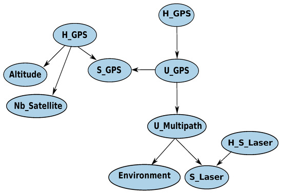
Figure 25.
BN GPS used for the parameters learning.
- H_GPS: represents the health of the GPS.
- H_S_GPS: represents the health of the GPS receiver.
- U_GPS: indicates the internal GPS type error node.
- S_GPS: represents the GPS receiver sensor.
- U_Multipath: indicates the multipath type error.
- S_Laser: laser sensor node.
- H_S_Laser: represents the health of of laser sensor.
- Nb_Satellite: indicates the number of the visible satellites.
- Altitude: indicates the altitude.
- Environment: represents the appearance context of multipath error.
Before applying the EM algorithm and learning the BN parameters, we need a learning database which can be built by simulation, mission history report, etc. For the GPS case study, we collect some information about a user position around an area (example: building) at different times. We consider a few known positions as a reference path. The difference between the computed position (using smartphone for example) and the reference one represent the GPS position deviation.
The information was collected at almost the same time over several days. The information recovered for each position located with GPSData application are: the latitude, the longitude and the altitude, the number of visible satellites and the accuracy of the position given by the GPS.
Each information collected by the user at different time corresponds to a specific node of the GPS monitor. Now, the collected data can be interpreted and transformed into BN data:
- Altitude correspond to ‘altitude’ node.
- Deviation correspond to ‘H_GPS’ node.
- Distance correspond to ‘S_laser’ node.
- Satellite correspond to ‘nb_satellite’ node.
- Accuracy correspond to ‘S_GPS’ node.
According to the value of the collected data and the fixed threshold for each node status of the GPS monitor. Thus, the data correspond to one of status of the corresponding BN node (interpreted as evidence). Table 8 shows how to interpret the real data into BN data.

Table 8.
Interpretation of raw data into BN node status.
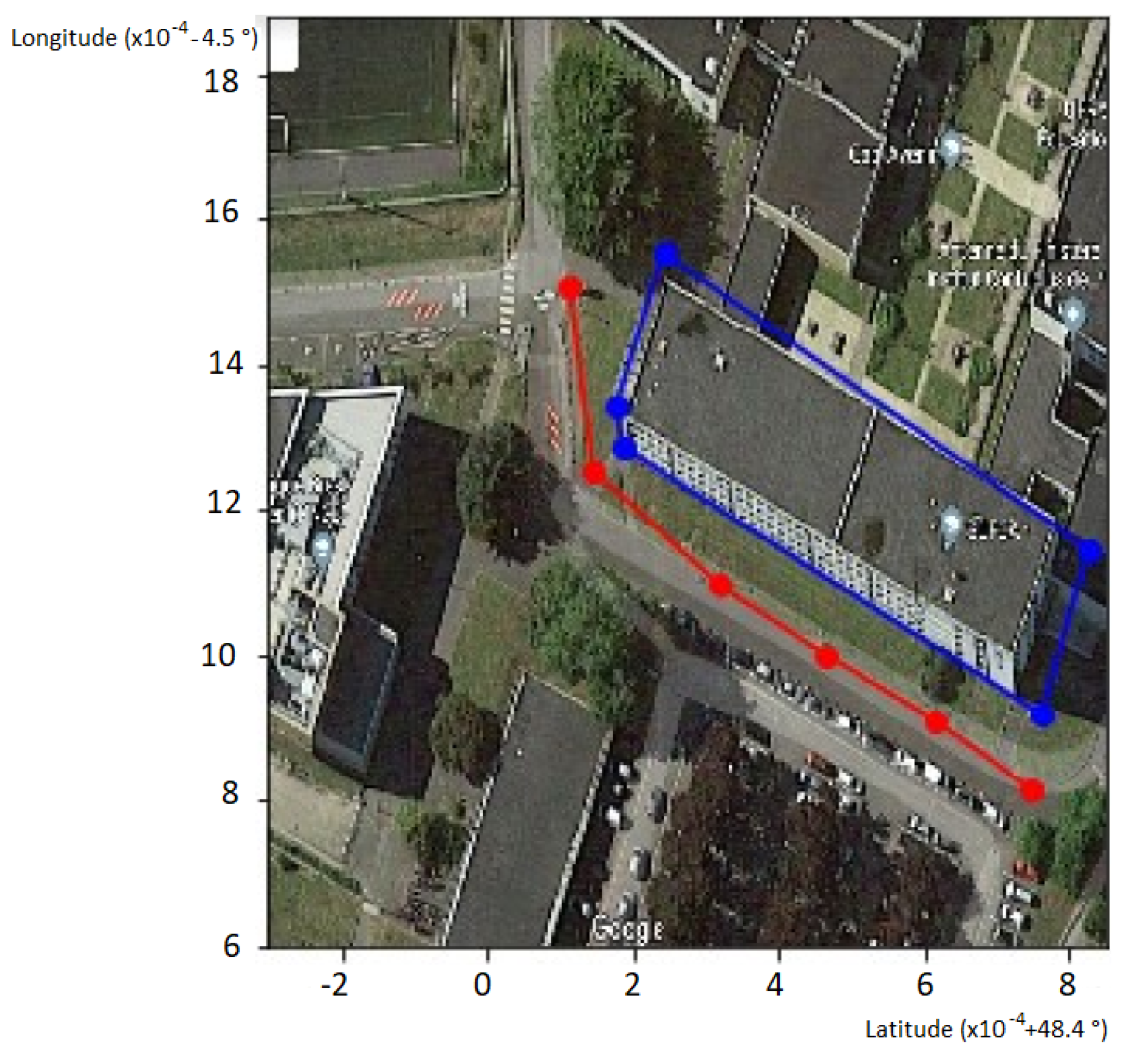
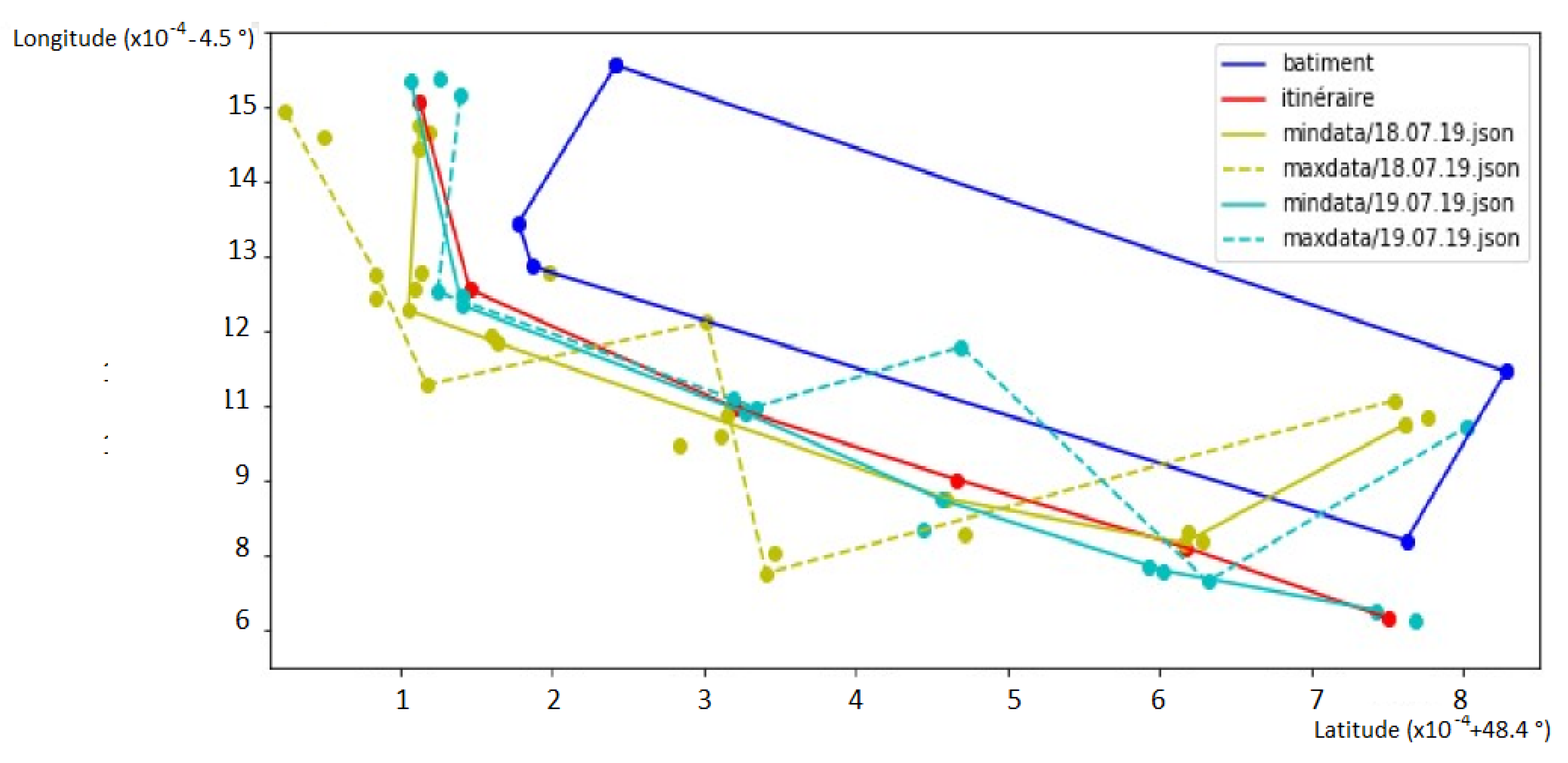
Once the database of the observed data for each node is built, we can perform the EM algorithm to learn the BN parameters which is the CPT probability values. The idea here is to compare the accuracy of the GPS position obtained with different collected database, with the reference one. Figure 26 shows the reference path (known position in red) around a building. Figure 27 shows the different paths (resulting from GPS positions) obtained by applying EM with different databases built from he collected data. In comparison with the reference path (in red on the figure), we can show that the accuracy of the GPS position varies according to the variation of the collected raw data and the rate of missing values in the database. In this case study, the parameters of all the BN nodes are learned with EM algorithm. The complexity of this approach varies according to the number of nodes and the conditional dependence. To deal with this, we can just learn the parameters of the pertinent nodes like the sensors nodes and the appearance context nodes using EM with another kind of inference mechanism [39].
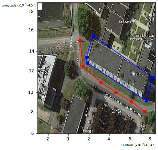
Figure 26.
Reference position (path) used.
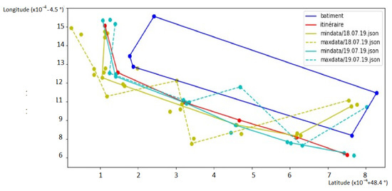
Figure 27.
Accuracy comparison between the reference path and the learned path.
6.2. HW/SW Implementation of Decision-Making Mechanism Based on BN
In the second part of the discussion, we look at the embedded version of the decision-making engine. In Section 4, we have evaluated the interest of a complete HW version in a case of decision-making engine using DN, we propose to extend this study with an MDP model. We focus on the implementation of decision-making part only in order to conclude for a strategy to adopt for elaborating an efficient embedded implementation.
HW Exploration of the MDP Model
To implement the BFM module, we can use a design flow very similar to the one defined in Figure 16 where the decision part is now expressed using an MDP model. The MDP part can be easily described in C-code and be mapped using HLS directives onto FPGA.
Table 9 shows the speed up obtained by executing the different MDPs describing the tracking mission phases (navigation, landing and tracking) on ZedBoard Xilinx and also the SW and HW execution time. We can see that the execution time increases according to the MDP size in terms of states and actions number. With a more complex mission than the tracking mission (with a hundred states and actions), the execution time and speed up increase significantly. For our case study, a response time lower than 10 ms is enough to apply the new mission plan generated by the decision module of BFM model. The Table 10 shows the resources needed for an HW implementation of the MDP part of the BFM.

Table 9.
MDP speed up and SW/HW execution time.

Table 10.
FPGA resources for the MDP implementations.
According to the results below, we can see the HW implementations of the MDP provide a short speed-up. The SW implementation of MDP can be enough for practical mission because low-latency decision-making mechanisms are most of the time enough for some practical mission cases. The HW resources can be used for other applications like vision-based ones. Nevertheless, the BN part of the BFM model can take benefit of an HW implementation as shown in Section 3.2.
Therefore, for an online execution of the mission planning, we can execute the diagnosis module on a hardware part (FPGA) and the decision module on a software part (CPU). This can be done either using a DN model or a BFM model for the decision-making mechanism. Nevertheless, in case of occupied CPU by the execution of other applications (obstacle detection, navigation, etc.), the HW implementation of the decision module (execution on FPGA) can be requested to unload the CPU and ensure the continuity of the on going mission.
7. Conclusions
The BN model is interesting to elaborate intelligent FDIR monitors incorporating the diagnosis and the error recovery modules. These ones can monitor the different elements of the system (sensors, hardware component, memories) but also the applications. Some system constraints (timing constraints and resources constraints) can also be introduced into these BN models. As the direct specification of the BN is not so easy, we propose a friendly method driven by pattern recognition and FMEA-like table specification to elaborate them. In a second part, we propose an efficient HW implementation of the BN monitors onto FPGA-SoC platform. The FPGA implementation can present a real interest for 2 reasons: speed-up and online updates. We give significative examples. We show with a BN monitor of 270 nodes that the corresponding FPGA implementation can offer a speed-up upto 16 compared to the SW version. It can be useful for a real-time monitoring. With an FPGA implementation, we are able to provide also non-intrusive monitors and we are able to perform the online updates by modifying the parameters of the networks, if necessary. Endly, the BN monitors can be incorporated into a decision-making model such as Decision Network or MDP to elaborate a high-level decision-making process of the mission manager. Embedded implementations of the cooperative diagnosis-decision making mechanism are also proposed on a FPGA-SoC support. We show that a co-design approach can provide an interesting trade-off for the decision-making implementation of the mission manager: diagnosis in HW and pure decision-making mechanism in SW. Actually, the BN monitors are the part that can mainly take benefit of an FPGA implementation while the decision-making mechanism is not so critical to be HW implemented.
As future works, we will consider the distributed approach of the BN monitors in a context of swarms including both the safety and the security constraints. In the case of a single drone, we have already explored a concurrent MDP specification incorporating BN monitors. This model can be applied for a cooperative mission between UAVs. Nevertheless, different challenges are still to be addressed. The first one concerns the adaptability of the UAV networks concerning a decision. This adaptability is necessary because the environmental context of the mission can change in real-time (strong wind, unexpected obstacle), because some security threats can be detected (GPS spoofing, deny of service, …), and because some failure may appear at different levels (sensor, motor, autopilot, companion board). To adapt the decision inside a swarm, we need to organize the global decision through the local ones. This means that the priorities should be fixed at the network level to make each single decision more appropriate and this must be done at real-time. Another challenge is the real-time feature that can be supported by an specific parallel hardware platform such as FPGA-SoC board. Our future work will propose a new methodology and new embedded implementations of the decision-making engine to be distributed onto a swarm in an adaptive and real-time way that includes the local monitors of each UAV. Predictions and learning are also under considerations to improve the BN monitoring and the decision-making.
Author Contributions
Conceptualization, C.D.; Methodology, C.D., S.Z., C.H.; Software, S.Z., C.H.; Validation, C.D., S.Z., C.H.; Formal analysis, C.D., S.Z., C.H.; Investigation, C.D., S.Z., C.H.; Writing original draft preparation, C.D.; Writing review and editing, C.D., S.Z., C.H.; Supervision, C.D.; Project administration, C.D.; Funding acquisition, C.D. All authors have read and agreed to the published version of the manuscript.
Funding
This research was funded by French CNRS (PICS SWARMS Project), by the French government and by French National Research (ANR), with the grant number ANR-10-LABX-07-01(RELIASIC Project) and the grant number ANR-15-CE24-0022-01 (HPeC Project).
Conflicts of Interest
The authors declare no conflict of interest.
References
- Avizienis, A.; Laprie, J.C.; Randell, B.; Landwehr, C. Basic concepts and taxonomy of dependable and secure computing. IEEE Trans. Dependable Secur. Comput. 2004, 1, 11–33. [Google Scholar] [CrossRef]
- Marzat, J.; Piet-Lahanier, H.; Damongeot, F.; Walter, E. Model-based fault diagnosis for aerospace systems: A survey. Proc. Inst. Mech. Eng. Part G J. Aerosp. Eng. 2012, 226, 1329–1360. [Google Scholar] [CrossRef]
- Wander, A.; Förstner, R. Innovative Fault Detection, Isolation and Recovery Strategies on-Board Spacecraft: State of the Art and Research Challenges; Deutsche Gesellschaft für Luft-und Raumfahrt-Lilienthal-Oberth eV: Bonn, Germany, 2013. [Google Scholar]
- Khakzad, N.; Khan, F.; Amyotte, P. Dynamic risk analysis using bow-tie approach. Reliab. Eng. Syst. Saf. 2012, 104, 36–44. [Google Scholar] [CrossRef]
- Khakzad, N.; Khan, F.; Amyotte, P. Safety analysis in process facilities: Comparison of fault tree and Bayesian network approaches. Reliab. Eng. Syst. Saf. 2011, 96, 925–932. [Google Scholar] [CrossRef]
- Bobbio, A.; Portinale, L.; Minichino, M.; Ciancamerla, E. Improving the analysis of dependable systems by mapping fault trees into Bayesian networks. Reliab. Eng. Syst. Saf. 2001, 71, 249–260. [Google Scholar] [CrossRef]
- Schumann, J.M.; Rozier, K.Y.; Reinbacher, T.; Mengshoel, O.J.; Mbaya, T.; Ippolito, C. Towards real-time, on-board, hardware-supported sensor and software health management for unmanned aerial systems. Int. J. Progn. Health Manag. 2015, 6, 021. [Google Scholar]
- Portinale, L.; Codetta-Raiteri, D. Arpha: An Fdir Architecture for Autonomous Spacecrafts Based On Dynamic Probabilistic Graphical Models. In Proceedings of the IJCAI workshop on AI on Space, Barcelona, Spain, 16–22 July 2011. [Google Scholar]
- Codetta-Raiteri, D.; Portinale, L. Dynamic Bayesian networks for fault detection, identification, and recovery in autonomous spacecraft. Syst. Man Cybern. Syst. IEEE Trans. 2015, 45, 13–24. [Google Scholar] [CrossRef]
- Schumann, J.; Moosbrugger, P.; Rozier, K.Y. R2U2: Monitoring and Diagnosis of Security Threats for Unmanned Aerial Systems; Springer: Cham, Switzerland, 2015; pp. 233–249. [Google Scholar]
- Muniraj, D.; Farhood, M. A framework for detection of sensor attacks on small unmanned aircraft systems. In Proceedings of the 2017 International Conference on Unmanned Aircraft Systems (ICUAS), Miami, FL, USA, 13–16 June 2017; pp. 1189–1198. [Google Scholar]
- Daly, R.; Shen, Q.; Aitken, S. Learning Bayesian networks: Approaches and issues. Knowl. Eng. Rev. 2011, 26, 99–157. [Google Scholar] [CrossRef]
- Grossman, D.; Domingos, P. Learning Bayesian Network Classifiers by Maximizing Conditional Likelihood. In Proceedings of the Twenty-first International Conference on Machine Learning, Banff, AB, Canada, 4–8 July 2004; p. 46. [Google Scholar] [CrossRef]
- Friedman, N. The Bayesian Structural EM Algorithm. In Proceedings of the Fourteenth Conference on Uncertainty in Artificial Intelligence, Madison, WI, USA, 24–26 July 1998; pp. 129–138. [Google Scholar]
- Chenini, H.; Heller, D.; Dezan, C.; Diguet, J.P.; Campbell, D. Embedded real-time localization of UAV based on an hybrid device. In Proceedings of the 2015 IEEE International Conference on Acoustics, Speech and Signal Processing (ICASSP), South Brisbane, QLD, Australia, 19–24 April 2015; pp. 1543–1547. [Google Scholar]
- Schumann, J.; Mengshoel, O.; Mbaya, T. Integrated Software and Sensor Health Management for Small Spacecraft. In Proceedings of the 2011 IEEE Fourth International Conference on Space Mission Challenges for Information Technology, Pasadena, CA, USA, 19–23 August 2011; pp. 77–84. [Google Scholar] [CrossRef]
- Geist, J.; Rozier, K.Y.; Schumann, J. Runtime Observer Pairs and Bayesian Network Reasoners On-board FPGAs: Flight-Certifiable System Health Management for Embedded Systems. In Proceedings of the Runtime Verification—5th International Conference, RV 2014, Toronto, ON, Canada, 22–25 September 2014; pp. 215–230. [Google Scholar] [CrossRef]
- Darwiche, A. A differential approach to inference in Bayesian networks. J. ACM 2003, 50, 280–305. [Google Scholar] [CrossRef]
- Cowell, R.G. Probabilistic Networks and Expert Systems: Exact Computational Methods for Bayesian Networks; Springer Science & Business: Medford, MA, USA, 2006. [Google Scholar]
- Zermani, S.; Dezan, C.; Hireche, C.; Euler, R.; Diguet, J.P. Embedded context aware diagnosis for a UAV SoC platform. Microprocess. Microsyst. 2017, 51, 185–197. [Google Scholar] [CrossRef]
- Zermani, S.; Dezan, C.; Diguet, J.; Euler, R. Bayesian Network-Based Framework for the design of Reconfigurable Health Management Monitors. In Proceedings of the NASA/ESA Conference on Adaptive Hardware and systems (AHS-15), Zhangjiajie, China, 18–20 November 2015. [Google Scholar]
- Zermani, S.; Dezan, C.; Chenini, H.; Diguet, J.; Euler, R. FPGA implementation of Bayesian network inference for an embedded diagnosis. In Proceedings of the 2015 IEEE Conference on Prognostics and Health Management (PHM), Austin, TX, USA, 22–25 June 2015; pp. 1–10. [Google Scholar]
- Xilinx. Available online: https://www.xilinx.com/support/documentation/sw_manuals/ug998-vivado-intro-fpga-design-hls.pdf. (accessed on 30 April 2020).
- Chavira, M.; Darwiche, A. Compiling Bayesian Networks with Local Structure. Available online: https://www.ijcai.org/Proceedings/05/Papers/0931.pdf (accessed on 30 April 2020).
- Tipaldi, M.; Glielmo, L. A survey on model-based mission planning and execution for autonomous spacecraft. IEEE Syst. J. 2017, 12, 3893–3905. [Google Scholar] [CrossRef]
- Druzdzel, M.J. SMILE: Structural Modeling, Inference, and Learning Engine and GeNIe: A Development Environment for Graphical Decision-Theoretic Models. Available online: https://www.aaai.org/Papers/AAAI/1999/AAAI99-129.pdf (accessed on 30 April 2020).
- Murphy, K. The Bayes Net Toolbox for MATLAB. Comput. Sci. Stat. 2001, 33, 2001. [Google Scholar]
- Kolobov, A. Planning with Markov decision processes: An AI perspective. Synth. Lect. Artif. Intell. Mach. Learn. 2012, 6, 1–210. [Google Scholar]
- Hireche, C.; Dezan, C.; Diguet, J.P.; Mejias, L. BFM: A Scalable and Resource-Aware Method for Adaptive Mission Planning of UAVs. In Proceedings of the 2018 IEEE International Conference on Robotics and Automation (ICRA), Brisbane, Australia, 21–25 May 2018; pp. 6702–6707. [Google Scholar]
- Hireche, C.; Dezan, C.; Mocanu, S.; Heller, D.; Diguet, J.P. Context/Resource-Aware Mission Planning Based on BNs and Concurrent MDPs for Autonomous UAVs. Sensors 2018, 18, 4266. [Google Scholar] [CrossRef] [PubMed]
- Zermani, S.; Dezan, C.; Hireche, C.; Euler, R.; Diguet, J.P. Embedded and probabilistic health management for the GPS of autonomous vehicles. In Proceedings of the 2016 5th Mediterranean Conference on Embedded Computing (MECO), Bar, Montenegro, 12–16 June 2016. [Google Scholar]
- Langley, R.B. The GPS error budget. GPS World 1997, 8, 51–56. [Google Scholar]
- Salós, D.; Macabiau, C.; Martineau, A.; Bonhoure, B.; Kubrak, D. Nominal GNSS pseudorange measurement model for vehicular urban applications. In Proceedings of the Position Location and Navigation Symposium (PLANS), 2010 IEEE/ION, Indian Wells, CA, USA, 4–6 May 2010; pp. 806–815. [Google Scholar]
- Dovis, F.; Muhammad, B.; Cianca, E.; Ali, K. A Run-Time Method Based on Observable Data for the Quality Assessment of GNSS Positioning Solutions. Sel. Areas Commun. IEEE J. 2015, 33, 2357–2365. [Google Scholar] [CrossRef]
- Drevelle, V.; Bonnifait, P. Reliable positioning domain computation for urban navigation. Intell. Transp. Syst. Mag. IEEE 2013, 5, 21–29. [Google Scholar] [CrossRef]
- Kalal, Z.; Mikolajczyk, K.; Matas, J. Tracking-Learning-Detection. IEEE Trans. Pattern Anal. Mach. Intell. 2012, 34, 1409–1422. [Google Scholar] [CrossRef] [PubMed]
- ZedBoard. Available online: http://zedboard.org/product/zedboard. (accessed on 30 April 2020).
- Tembo, S.R.; Vaton, S.; Courant, J.L.; Gosselin, S. A tutorial on the EM algorithm for Bayesian networks: Application to self-diagnosis of GPON-FTTH networks. In Proceedings of the 2016 International Wireless Communications and Mobile Computing Conference (IWCMC), Paphos, Cyprus, 5–9 September 2016; pp. 369–376. [Google Scholar]
- Hireche, C.; Dezan, C.; Diguet, J.P. Online diagnosis updates for embedded health management. In Proceedings of the 2017 6th Mediterranean Conference on Embedded Computing (MECO), Bar, Montenegro, 11–15 June 2017; pp. 1–5. [Google Scholar]
- Lauritzen, S.L. The EM algorithm for graphical association models with missing data. Comput. Stat. Data Anal. 1995, 19, 191–201. [Google Scholar] [CrossRef]
© 2020 by the authors. Licensee MDPI, Basel, Switzerland. This article is an open access article distributed under the terms and conditions of the Creative Commons Attribution (CC BY) license (http://creativecommons.org/licenses/by/4.0/).


