Approximate Triangulations of Grassmann Manifolds


Abstract
1. Introduction
2. Materials and Methods
2.1. Grassmann Manifolds
2.2. Schubert Cells
| 0 | |
| 1 | |
| 2 | |
| 2 | |
| 3 | |
| 4 |
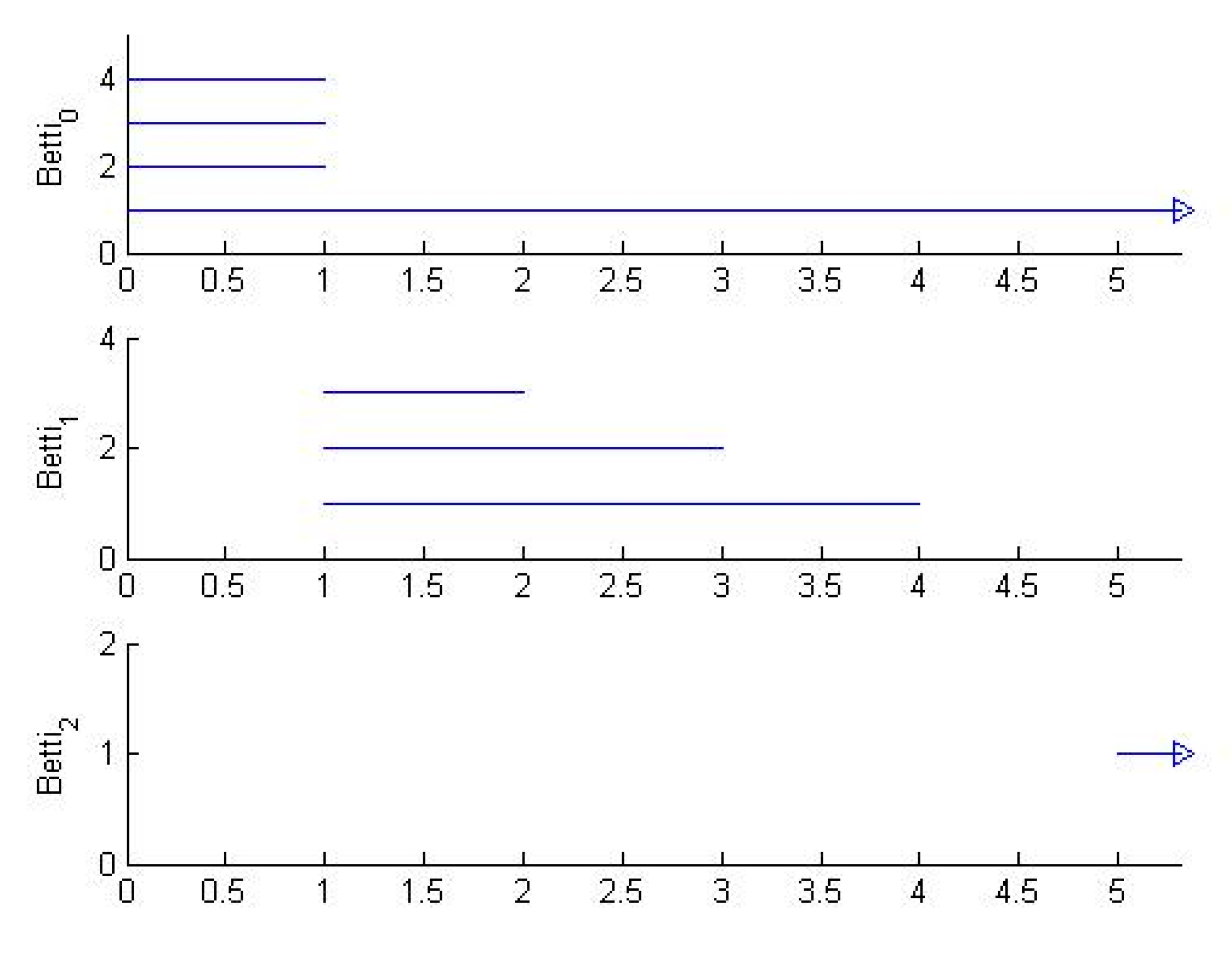
2.3. Persistent Homology
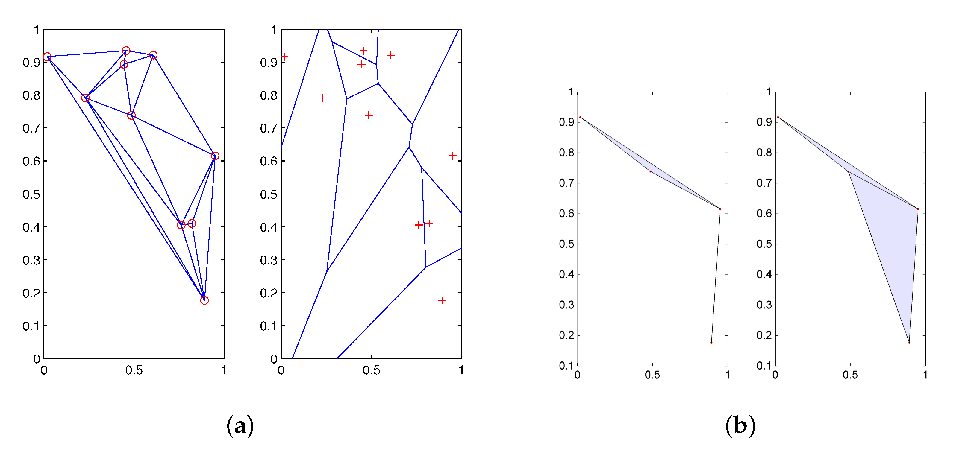
2.4. Vietoris–Rips and Witness Complexes
- •
- The vertex set of is L;
- •
- span an edge if there exists an , called a witness, such that
- •
- A collection spans a p-simplex if span an edge for all .
- If , then form an edge if there is an such that and are the two smallest entries in the i-th column of D. This is analogous to the existence of an edge in the Delaunay triangulation .
- For , one may think of relaxing the boundaries of the Voronoi diagram of L and taking the nerve of the resulting covering of X.
- If , then there is an inclusion of simplicial complexes .
- How should the landmark set L be chosen?
- What is the correct value of R?
- Select landmarks at random.
- Use the maxmin procedure: Choose a seed at random. Then, if have been chosen, let be the point which maximizes the function
- Use a density-based strategy.
2.5. Sampling Procedures
- Select k random vectors in .
- Perform the Gram–Schmidt orthogonalization algorithm to yield an orthornomal set . Let A be the matrix with as columns.
- Compute .
- Determine the percentage of sample points desired from each Schubert cell. For example, one might choose 5% from a 1-cell, 10% from a 2-cell, and so on.
- Elements of a given Schubert cell correspond to the column space of a particular matrix form. Generate such a matrix B using random vectors of the required form.
- Generate a random orthogonal matrix X.
- Add the matrix to the point cloud.
2.6. Approximate Triangulations
- Construct a sample of points on .
- Construct a collection of Vietoris–Rips or witness complexes on the point cloud.
- Compute the persistent homology of this filtration.
- Determine a range of parameters where the homology of the complexes agrees with that of .
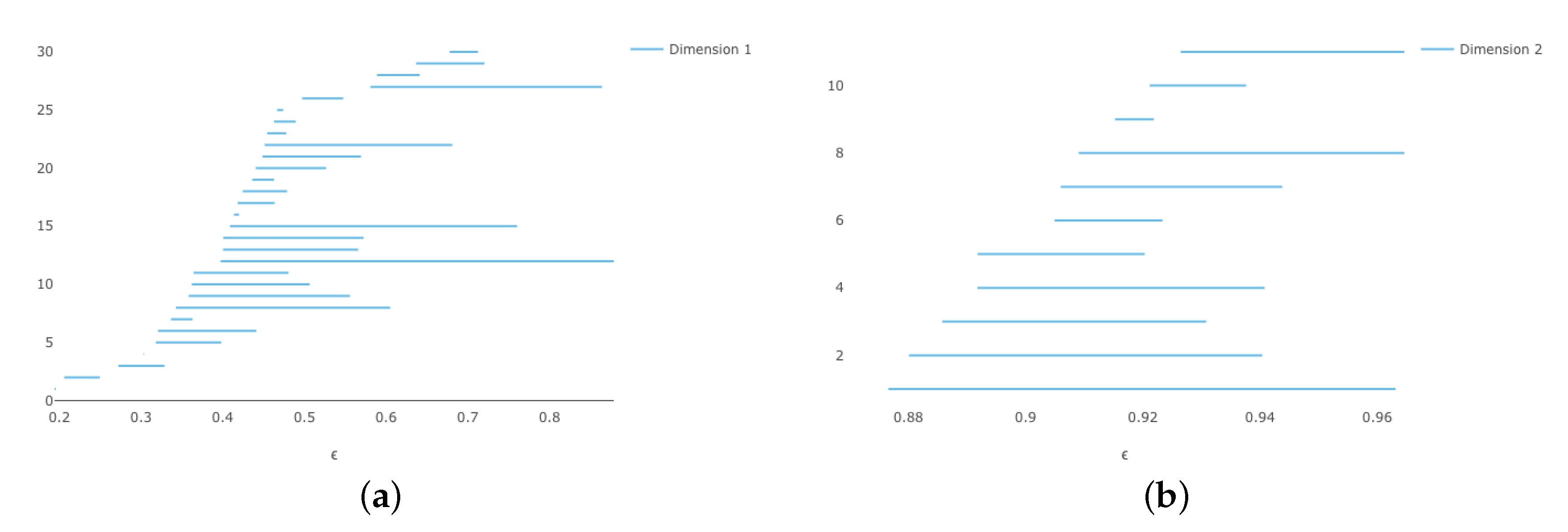
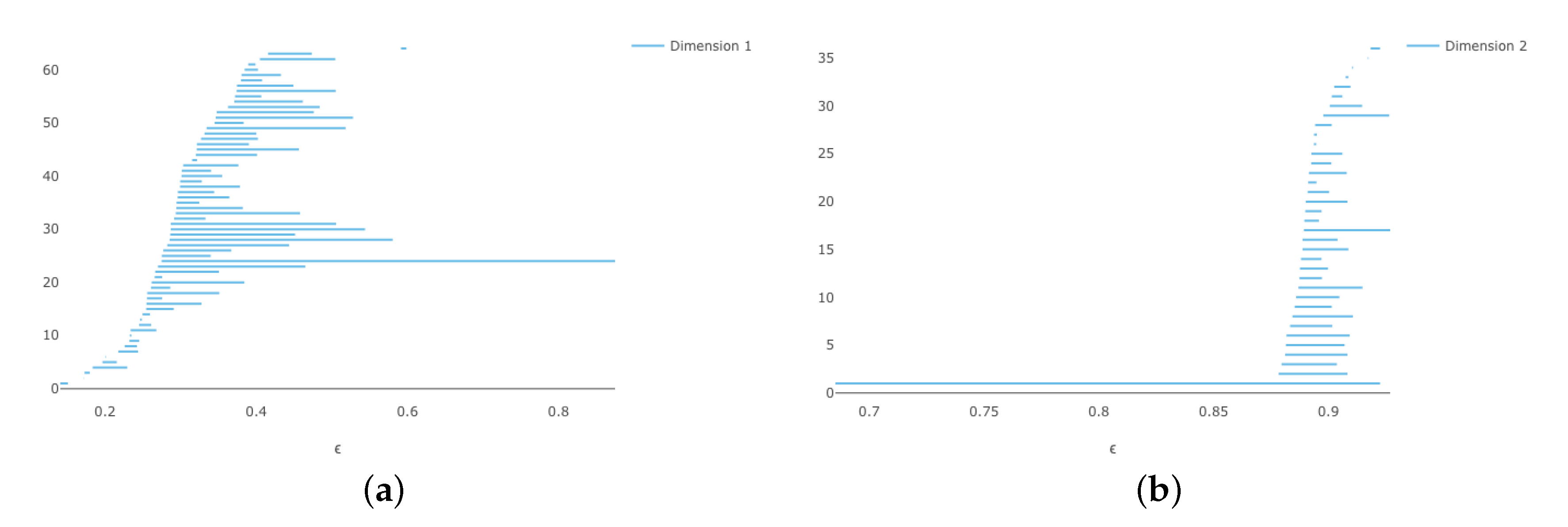
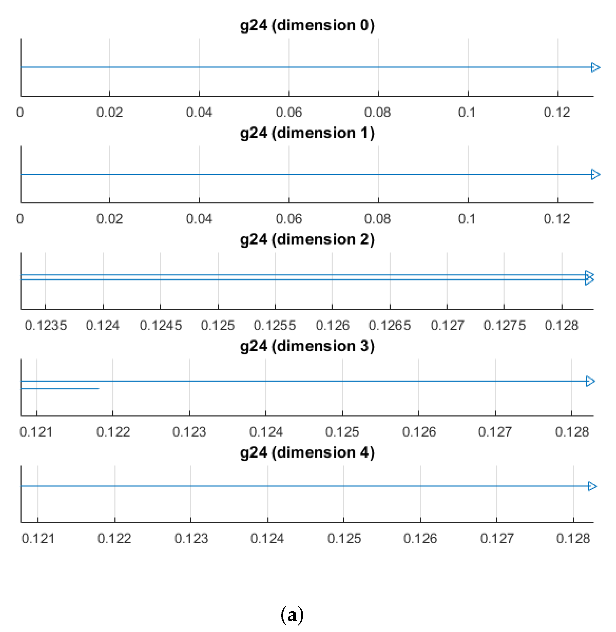
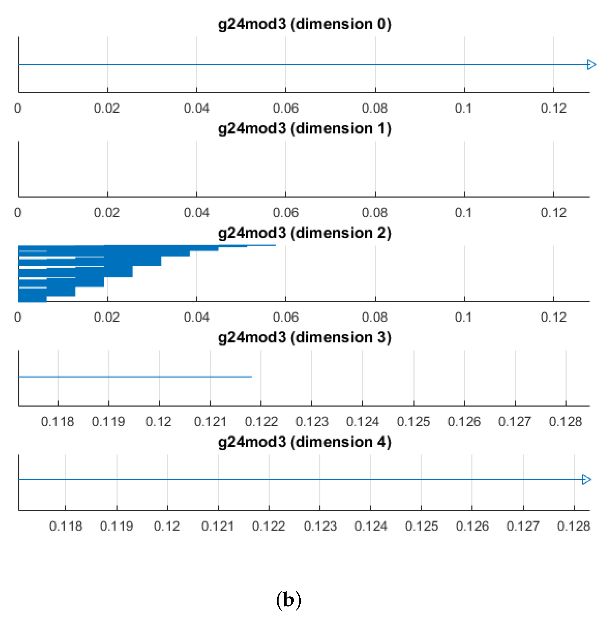
3. Results
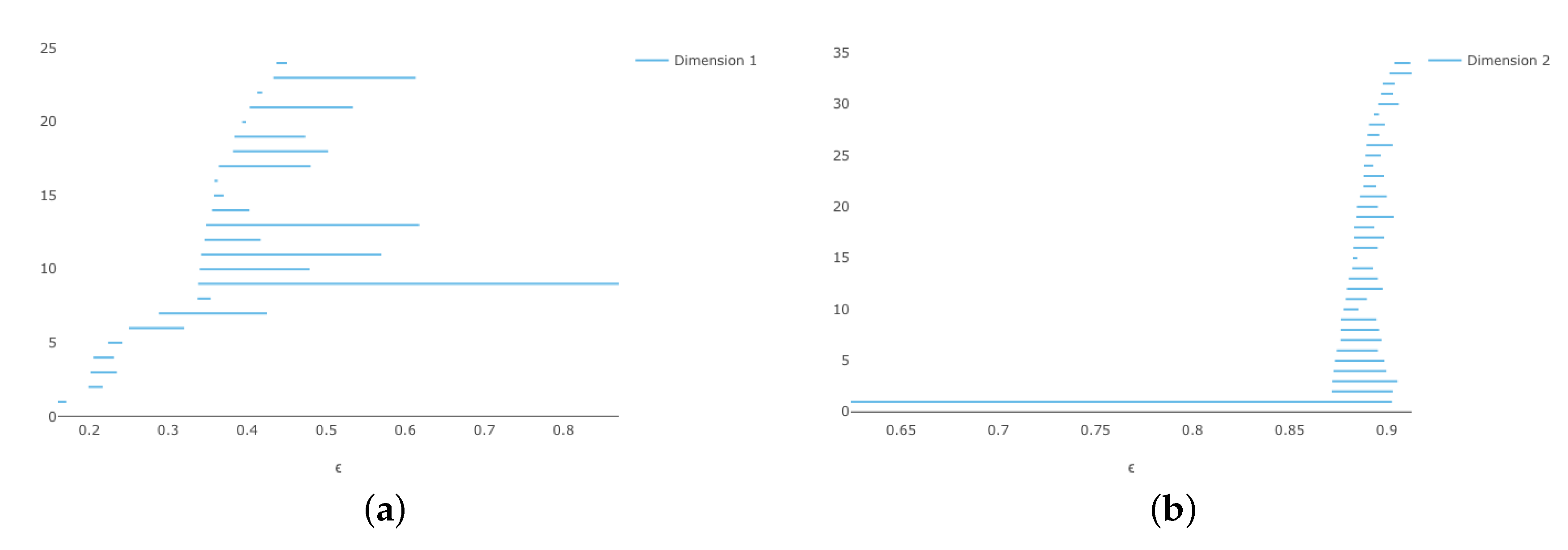
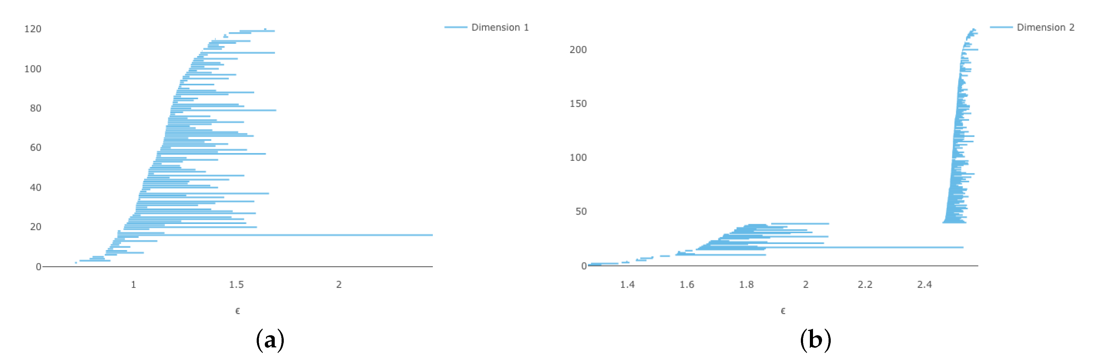
3.1. , Part I
3.2. , Part II
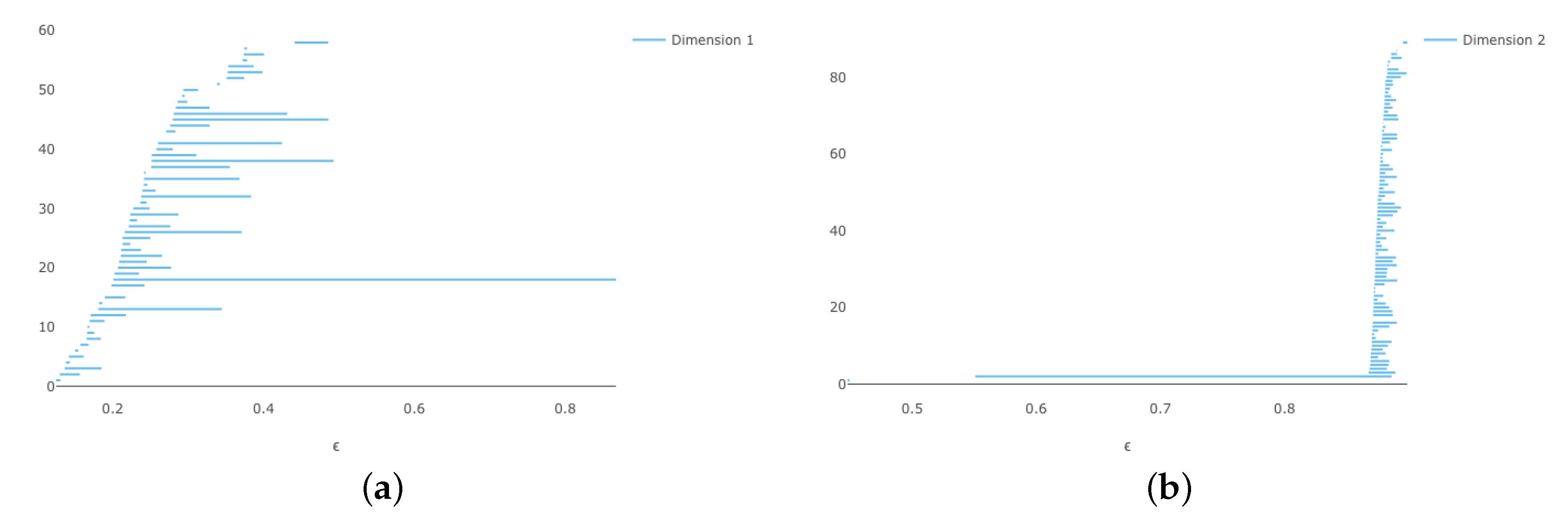
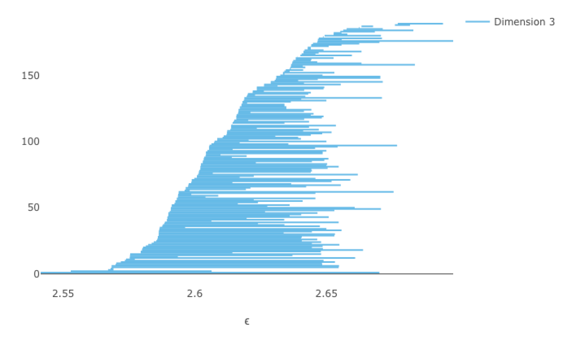
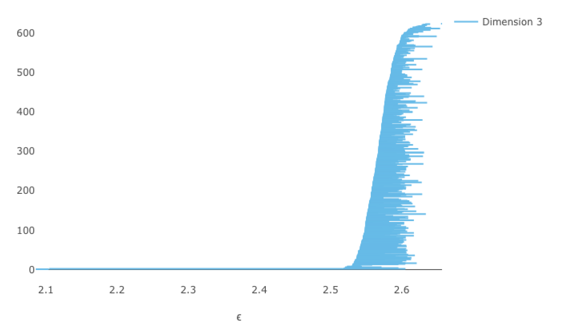
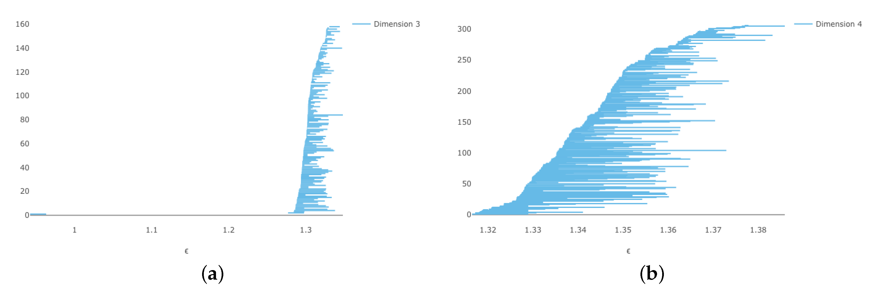
3.3.
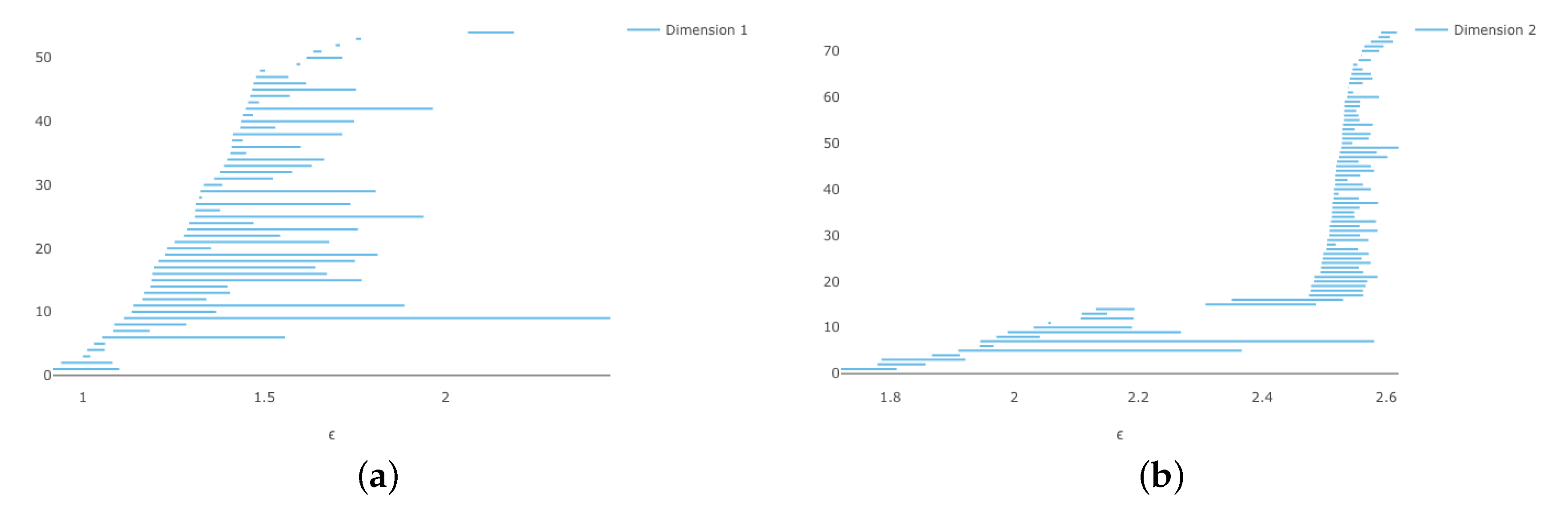
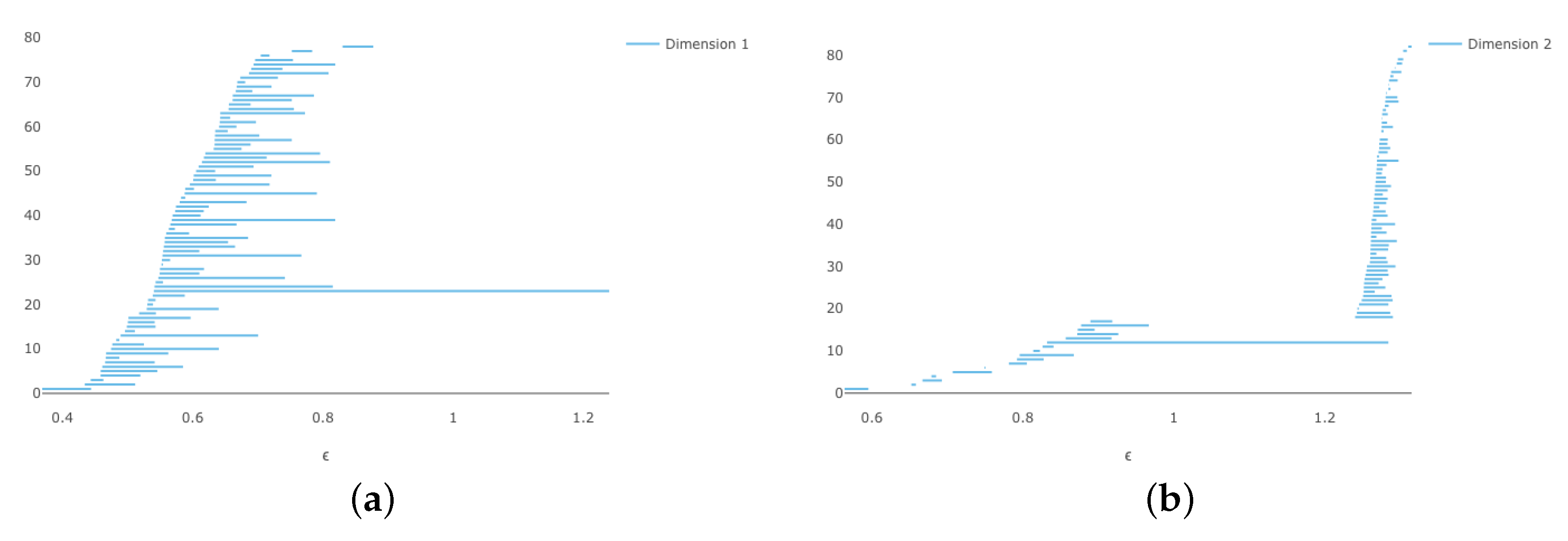
3.4. , Part I
3.5. , Part II
4. Conclusions
- How small of a sample can we use to generate an approximate triangulation? For example, a result in [3] asserts that any triangulation of must have at least 14 vertices. We built an approximate triangulation using a witness complex on 100 landmarks. Surely, our algorithm will not work with only 14 points, but we plan to investigate how few we can get away with. A theorem of Niyogi–Smale–Weinberger [16] provides lower bounds on the number of points required to compute homology correctly with high probability, but these are certainly too high and can be improved in practice.
- Can we push the computations further? The next Grassmannian to study is . This is a nonorientable 6-manifold, and, using our procedure, we would embed it in . The machine used to compute the persistent homology of the witness complexes on in MATLAB ran out of memory on 100 landmarks in . We therefore need either a bigger machine running MATLAB, or software that can handle witness complexes. The GUDHI package [17] is one option, but we have not attempted it yet.
- The author expects to gain access to a new GPU based supercomputer at his institution in the next year. This may allow for similar computations on higher-dimensional .
Funding
Acknowledgments
Conflicts of Interest
References
- Whitehead, J. On C1-complexes. Ann. Math. 1940, 41, 809–824. [Google Scholar] [CrossRef]
- Duan, H.; Marzantowicz, W.; Zhao, X. Estimate of number of simplices of triangulations of Lie groups. arXiv 2020, arXiv:2003.13125. [Google Scholar]
- Govc, D.; Marzantowicz, W.; Pavešić, P. How many simplices are needed to triangulate a Grassmannian? arXiv 2020, arXiv:2001.08292. [Google Scholar]
- Milnor, J.; Stasheff, J. Characteristic Classes; Annals of Mathematics Studies 76; Princeton University Press: Princeton, NJ, USA, 1974. [Google Scholar]
- Anderson, L.; Davis, J. There is no tame triangulation of the infinite real Grassmannian. Adv. Appl. Math. 2001, 26, 226–236. [Google Scholar] [CrossRef]
- Aanjaneya, M.; Teillaud, M. Triangulating the real projective plane. MACIS Proc. 2007. preprint version. Available online: https://arxiv.org/abs/0709.2831 (accessed on 16 July 2020).
- Casian, L.; Kodama, Y. On the Cohomology of Real Grassmann Manifolds. 2013. preprint. Available online: https://arxiv.org/abs/1309.5520 (accessed on 22 June 2020).
- Henselman, G. Eirene, a Software Package for Computing Persistent Homology. Available online: https://github.com/Eetion/Eirene.jl (accessed on 22 June 2020).
- Bauer, U. Ripser, a Software Package for Computing Persistent Homology. Available online: https://github.com/Ripser/ripser (accessed on 22 June 2020).
- Nanda, V. Perseus, the Persistent Homology Software. Available online: http://www.sas.upenn.edu/~vnanda/perseus (accessed on 22 June 2020).
- De Silva, V.; Carlsson, G. Topological estimation using witness complexes. In Eurographics Symposium on Point-Based Graphics; A.K. Peters: Wellesley, MA, USA, 2004. [Google Scholar]
- Chazal, F.; Oudot, S. Towards persistence-based reconstruction in Euclidean spaces. In Proceedings of the 24th ACM Symposium on Computational Geometry, College Park, MD, USA, 9–11 June 2008; pp. 232–241. [Google Scholar]
- Davis, D. Embeddings of real projective spaces. Bol. Soc. Mat. Mex. 1998, 4, 115–122. [Google Scholar]
- Zhang, Y. Isometric embeddings of real projective spaces into Euclidean spaces. Differ. Geom. Appl. 2009, 27, 100–103. [Google Scholar] [CrossRef]
- JavaPlex Persistent Homology and Topological Data Analysis Library. Available online: http://appliedtopology.github.io/javaplex/ (accessed on 22 June 2020).
- Niyogi, P.; Smale, S.; Weinberger, S. Finding the homology of submanifolds with high confidence from random samples. Disc. Comp. Geom. 2008, 39, 419–441. [Google Scholar] [CrossRef]
- GUDHI: Geometry Understanding in Higher Dimensions. Available online: https://gudhi.inria.fr/ (accessed on 22 June 2020).


| Space | # Points | Top Dim | # Simplices | Eirene | Ripser |
|---|---|---|---|---|---|
| 100 | 2 | 206K | 0:00.53 | – | |
| 200 | 2 | 2.1M | 0:01 | – | |
| 100 | 2 | 436K | 0:02 | – | |
| 200 | 2 | 4.2M | 0:07 | – | |
| 100 | 3 | 7.6M | 0:09 | – | |
| 200 | 3 | 146M | 6:54 | – | |
| 100 | 4 | 107M | 1:51 | 1:15 | |
| 150 | 4 | 792M | 1:04:45 | X | |
| 200 | 3 | 112M | 3:01 | 3:07 | |
| 200 | 4 | ? | X | X |
© 2020 by the author. Licensee MDPI, Basel, Switzerland. This article is an open access article distributed under the terms and conditions of the Creative Commons Attribution (CC BY) license (http://creativecommons.org/licenses/by/4.0/).
Share and Cite
Knudson, K.P. Approximate Triangulations of Grassmann Manifolds. Algorithms 2020, 13, 172. https://doi.org/10.3390/a13070172
Knudson KP. Approximate Triangulations of Grassmann Manifolds. Algorithms. 2020; 13(7):172. https://doi.org/10.3390/a13070172
Chicago/Turabian StyleKnudson, Kevin P. 2020. "Approximate Triangulations of Grassmann Manifolds" Algorithms 13, no. 7: 172. https://doi.org/10.3390/a13070172
APA StyleKnudson, K. P. (2020). Approximate Triangulations of Grassmann Manifolds. Algorithms, 13(7), 172. https://doi.org/10.3390/a13070172