An Algorithm for Density Enrichment of Sparse Collaborative Filtering Datasets Using Robust Predictions as Derived Ratings

Abstract

Collaborative filtering algorithms formulate personalized recommendations for a user, first by analysing already entered ratings to identify other users with similar tastes to the user (termed as near neighbours), and then using the opinions of the near neighbours to predict which items the target user would like. However, in sparse datasets, too few near neighbours can be identified, resulting in low accuracy predictions and even a total inability to formulate personalized predictions. This paper addresses the sparsity problem by presenting an algorithm that uses robust predictions, that is predictions deemed as highly probable to be accurate, as derived ratings. Thus, the density of sparse datasets increases, and improved rating prediction coverage and accuracy are achieved. The proposed algorithm, termed as CF_DR, is extensively evaluated using (1) seven widely-used collaborative filtering datasets, (2) the two most widely-used correlation metrics in collaborative filtering research, namely the Pearson correlation coefficient and the cosine similarity, and (3) the two most widely-used error metrics in collaborative filtering, namely the mean absolute error and the root mean square error. The evaluation results show that, by successfully increasing the density of the datasets, the capacity of collaborative filtering systems to formulate personalized and accurate recommendations is considerably improved.

1. Introduction

Collaborative filtering (CF) algorithms formulate personalized recommendations by taking into account users’ ratings that denote their interests and tastes. Initially, these algorithms identify the users that have highly similar interests and tastes with the user for whom the recommendation will be formulated. These users are called “near neighbours” (NNs). Then, their ratings are used in order to formulate rating predictions which will subsequently result in the formulation of recommendations [1,2].

However, in sparse CF datasets, i.e., datasets that contain small number of ratings, compared to the number of users and items, the quality of recommendations is degraded, since (a) in many cases a CF recommender system (RS) either cannot compute predictions for certain users due to lack of NNs (a phenomenon termed as the “grey sheep” problem), thus reducing prediction coverage (i.e., percentage of the users for whom personalized predictions can be computed) and (b) for users that have a low number of NNs, the computed predictions have low accuracy [3]. The current literature includes numerous research efforts aiming to tackle the data sparsity problem. To this end, most works exploit different types of additional information (i.e., information beyond the rating matrix), such as social relationships between users, item descriptions, textual reviews for items and so forth (a detailed review is given in Section 2). However, such information is not always available or exploitable (e.g., due to lack of user consent).

This paper addresses the aforementioned problems by:

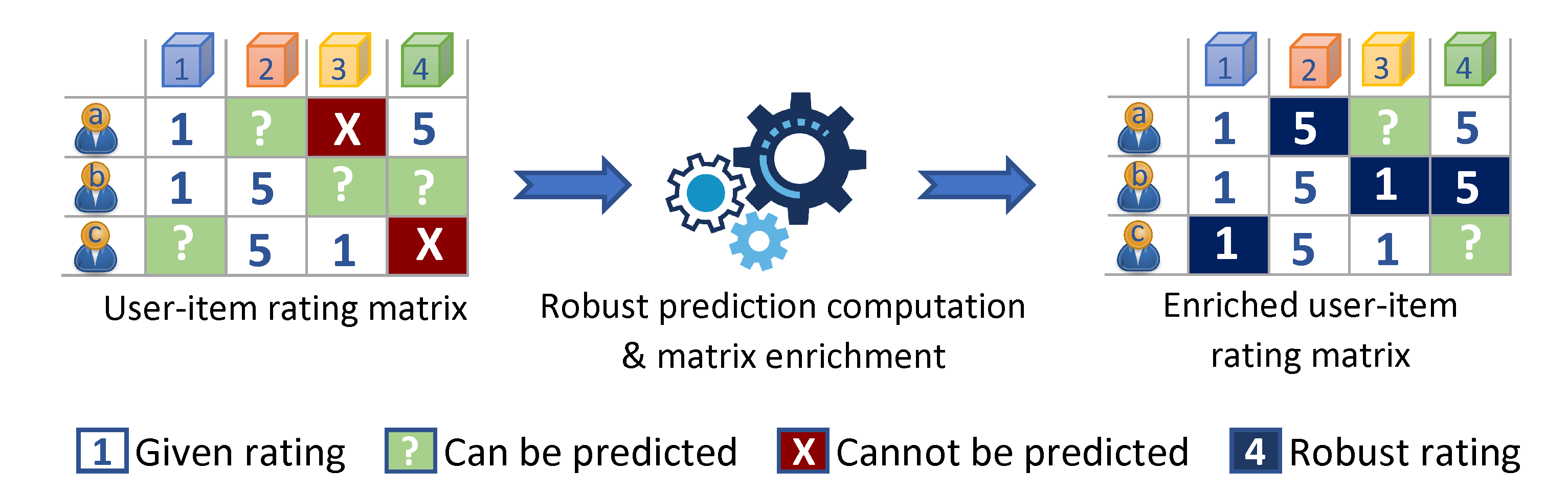
• Introducing the concepts of derived ratings (DRs) and robust predictions: derived ratings are created from predictions with a high level of confidence regarding their accuracy, which are termed as robust predictions. DRs complement the explicitly entered ratings in the user–item rating matrix, increasing the matrix density.
• Proposing an algorithm, termed CF_DR, for the creation of DRs on the basis of real, explicit user ratings, while considering various prediction robustness criteria.
• Extending the rating prediction computation algorithm to compute rating predictions on the complemented user-item rating matrix, while taking into account the level of confidence associated with each DR.

The algorithm proposed in this paper outperforms all algorithms presented in the literature that target the data sparsity problem and rely only on the data included in the rating matrix, both in terms of being able to formulate personalized recommendations and increasing rating prediction accuracy. Additionally, the proposed approach can be combined with algorithms and techniques that exploit additional data and/or use different prediction computation approaches.

To exemplify the concept of the CF_DR algorithm, let us consider the case where we want to predict the rating r_U3,i4 that user U₃ would assign to item i₄, in order to decide whether it should be recommended to him or not. Let us also assume that the RS computes user similarity using the Pearson correlation coefficient [1,2] and that, at rating prediction time, the user–item ratings database is as depicted in

Table 1. User-item rating database excerpt.

User/Item	i1	i2	i3	i4	i5
U1	1			5
U2	1	5
U3		5	1
U4					5

.

In this setting, a prediction for grey-shaded cells cannot be computed, due to the fact that the corresponding user has no near neighbours that have rated the particular item. Considering, for instance, cell (U₃, i₄), a prediction for r_U3,i4 cannot be computed, since: (1) U₃ has only one NN, U₂ (they share a positive correlation with each other, since they have both rated item i₂ with a high score), but U₂ has not rated item i₄, and (2) although user U₁ has rated item i₄, he does not belong to U₃′s NN set (no common rated items). The case for cell (U₁, i₃) is similar while, notably, U₄ has not rated any item in common with other users, and i₅ has only been rated by U₄, Hence, no rating prediction can be formulated for any item for U₄, and no rating prediction can be computed for any user regarding item i₅.

However, we can also observe in Table 1 that users U₁ and U₂ are NNs with each other (they share a positive correlation, having both rated item i₁ with a low score) and hence if U₂ had asked for a prediction on item i₄ (instead of user U₃) that prediction could have been formulated.

According to the CF_DR algorithm proposed in this paper, a preprocessing step is executed that computes all the predictions that can be formulated for all the users in the CF rating database, and the predictions having a high level of confidence regarding their accuracy, i.e., the robust ones, are converted to DRs and stored into the user-item ratings database.

Table 2. User-item rating database excerpt after the execution of the preprocessing step of CF_DR.

User/Item	i1	i2	i3	i4	i5
U1	1	5		5
U2	1	5	1	5
U3	1	5	1
U4					5

depicts the state of the user-item rating matrix from Table 1 after the execution of the preprocessing step of the CF_DR algorithm (the newly inserted DRs are shown in bold).

We can observe that the user-item rating matrix is now considerably denser. Its density, computed as $\frac{\#ratings}{\#items\times \#users}$, has increased from 0.35 to 0.55 and, due to this increase, the prediction for the ratings r_U3,i4 and r_U3,i3 can now be formulated. The ability to compute rating predictions that could not be formulated on the basis of the original user-item rating matrix stems from the two following properties of the DR-enriched -item rating matrix:

In the DR-enriched item rating matrix, the near neighbourhood of a user U may extend to accommodate a set of additional users ${\mathrm{NN}}_{\mathrm{U}}^{\mathrm{New}}$. The ratings of the users in the set ${\mathrm{NN}}_{\mathrm{U}}^{\mathrm{New}}$ can be exploited to compute rating predictions that could not have been computed on the basis of the original user-item rating matrix. Indeed, we can observe that, due to the addition of DRs r_U3,i2 and r_U3,i1 in the DR-enriched database depicted in Table 2, U₃′s near neighbourhood has extended to include U₁, hence any rating recorded by U₁ can now be used for computing rating predictions for U₃, as is the case with r_U3,i4. It is worth noting at this point that the ability to compute a prediction for r_U3,i4 can lead to the formulation of a personalized recommendation for user U₃: in the situation depicted in Table 1, only the value of r_U3,i1 could be predicted. However, this value is very low (1) and hence i₁ would not be recommended to U₃. Then, the recommendation algorithm would either refrain from formulating a recommendation or use the mean database rating value for items i₄ and i₅, which is 5 for both items, and therefore would arbitrarily choose among them. In the DR-enriched rating matrix context, the recommendation algorithm has a prediction for rating r_U3,i4 at its disposal and can therefore knowledgably select and recommend i₄ to U₃.

In the DR-enriched item rating matrix, already existing near neighbours of a user U can contribute more ratings when rating predictions for user U are calculated, therefore it is possible to compute predictions regarding U’s ratings on items, which could not have been computed on the basis of the original user-item rating matrix. Indeed, we can observe that, due to the addition of DR r_U3,i3, user U₂, who was formerly a NN of U₁, can now contribute to the computation of a rating prediction for r_U3,i3. Regarding the recommendation formulation stage, when the RS utilises the DR-enriched rating matrix the recommendation algorithm, having at its disposal a prediction for rating r_U3,i3, it can knowledgeably refrain from recommending item i₃ to U₁, rather than relying on the database rating mean value for this item.

Regarding user U₄, who had no common ratings with any other user in the user-item rating matrix, still no near-neighbours can be identified for him/her in the context of the DR-enriched user-item rating matrix. Similarly, in the same context, no personalized prediction can be computed for item i₅. These cases mainly correspond to the cold start problem [4,5]. The cold start problem can be tackled using content-based algorithms [6,7], context-based algorithms [8], and social network-based algorithms [9,10]. Each class of such algorithms requires additional information, while it is also possible that such algorithms are combined with the approach presented in this paper.

In the example presented above, for simplicity, each rating prediction was considered to be robust and hence produced a DR. However, this setting may not be the optimal one. The optimal setting for tuning the algorithm operation, regarding the characterization of predictions as robust, is presented in Section 4. Notably, the procedure employed in Section 4 follows a grid search approach to hyperparameter tuning. Since hyperparameters moderate the importance of various robustness estimators (e.g., number and similarity of contributing NNs), alternative methods can be employed for combining the partial estimators to optimize the prediction model, such as merging estimators [11,12,13].

In order to validate the CF_DR algorithm, an extensive evaluation is conducted, assessing (1) the degree of density enrichment, (2) the prediction coverage increase, and (3) the prediction accuracy increase, achieved by the proposed algorithm. In this evaluation, we use seven contemporary and widely used CF datasets from various domains (videogames, music, movies, food, etc.). We consider the two most widely used CF similarity metrics, namely the Pearson correlation coefficient and the cosine similarity and the two most widely used CF error metrics, namely the mean average error and the root mean square error.

Finally, it is worth noting that the CF_DR algorithm, proposed in this paper, can be combined with other works in the domain of CF, targeting either to (1) enhance rating prediction accuracy [14,15,16,17], (2) improve recommendation quality [18,19,20,21], (3) increase rating prediction computation efficiency [22,23,24,25], or (4) further increase prediction coverage in CF-based RSs [26,27,28,29].

The rest of the paper is structured as follows: Section 2 overviews the related work, while Section 3 introduces the CF_DR algorithm. Section 4 reports on the methodology for tuning the algorithm operation and evaluates the presented algorithm. Finally, Section 5 discusses the experimental results and presents a comparison with state-of-the-art algorithms addressing the sparsity issue, while Section 6 concludes the paper and outlines future work.

2. Related Work

CF-based RS prediction accuracy is a field that has attracted significant research efforts over the last years [30,31,32]. In contrast, research in CF-based RS coverage is less developed.

Vozalis et al. [33] present ItemHyCov, which is a CF-based prediction algorithm that combines the strengths of user-based and item-based CF approaches into a feature combination hybrid CF approach, targeting to upgrade the CF rating prediction coverage in sparse CF datasets. In order to achieve its goals, the ItemHyCov algorithm introduces a preprocessing hybrid combination step. However, it necessitates both extra preprocessing time and extra storage space, as well as continuous updates. The CF_negNNs algorithm presented in [26] increases the CF rating prediction coverage in sparse datasets, by incorporating, in the rating prediction computation process, users with negative similarity to the user for whom the rating prediction is computed. Margaris et al. [27] propose the CF_VNN algorithm, which creates virtual user profiles, termed virtual NNs (VNNs), by merging pairs of NN profiles corresponding to real users having high similarity. The introduction of the VNN profiles contributes to the alleviation of the “grey sheep” problem. Additionally, Margaris and Vassilakis [29] present an algorithm, termed CF_FOAF, which adopts the friend-of-a-friend concept in CF, in the sense that two users can be considered as NNs with each other if they are NNs to a third user. Effectively, the CF_FOAF algorithm explores the effect of considering transitivity of the NN relationships, examining different parameters of computing properties of the derived relationships.

Pham et al. [24] present a clustering CF recommendation algorithm that exploits social relationships between social network (SN) users to identify their social neighbourhoods. It applies a complex network clustering technique on the SN users to formulate similar user groups and, then, uses traditional CF algorithms to generate the recommendations. Wang et al. [34] combine CF techniques with user trust relationships and put forward the recommendation approach based on trust delivery, in order to solve the data sparsity and cold-start problems that the sparse CF datasets suffer from. Jiang et al. [35] propose an algorithm which fuses trusted rating data (i.e., rating data that have been upvoted by community users as “helpful”) with user similarity and, subsequently, applies an improved version of the slope one algorithm to generate rating predictions. The proposed algorithm comprises three procedures, namely the selection of trusted data, similarity calculation between users, and weight factor addition to the aforementioned similarity, in order to create the recommendation equation. Zarei and Moosavi [36] propose a social memory-based CF algorithm and examine the impact of integrating social ties on both prediction coverage and accuracy. Moreover, in order to tune the contribution of SN information, the proposed algorithm incorporates a learning method as a weight parameter in the proposed similarity measure. Margaris et al. [37] propose an algorithm that targets SN RSs that operate using sparse user-item rating matrices, as well as sparse social graphs. For each user-item prediction, the proposed algorithm computes partial predictions for item ratings from both the user’s CF neighbourhood and SN neighbourhood, which are then combined using a weighted average technique. The weight is adjusted to fit the characteristics of the dataset. For users that have no CF or SN NNs, item predictions are based only on the respective user’s social neighbourhood or CF neighbourhood, respectively. All the aforementioned approaches significantly improve CF rating prediction coverage. However, the improvement is based on information derived from complementary information sources (e.g., a SN), which is not always available.

Matrix factorization (MF) algorithms [38,39] constitute an alternative category for computing rating predictions. However, since the MF-based approaches always produce a rating prediction when these algorithms are applied to sparse datasets, the predictions involving items or users having very few ratings actually degenerate to dataset-dependent constant values, which are not considered as personalized predictions. Furthermore, the rating prediction accuracy of these algorithms is relatively poor in these cases [40,41]. Guan et al. [42] address this issue by proposing an upgraded singular value decomposition (SVD) model that incorporates the MF algorithms with rating completion inspired by active learning, as well as a multi-layer ESVD model that further improves rating prediction accuracy. Moreover, Braunhofer et al. [43] present the benefits of using active learning techniques and the users’ personalities and develop two extended MF algorithm versions to identify the items a user could and should rate, as well as compose personalized recommendations. Kalloori et al. [44] propose a MF and a NN prediction technique for pairwise preference scores. The MF-based algorithm maps user and item pairs to a joint latent feature vector space, whereas the respective NN method employs custom user-to-user similarity functions, which are identified as more accurate for synthesizing user rating values into a user similarity metric. Luo et al. [45] propose an approach for building a nonnegative latent factor (NLF) model, which is based on the alternating direction method. This method substitutes direct matrix manipulations by training the desired features through single-element-dependent optimisation, reaping considerable benefits in computational complexity and storage space, while also achieving accuracy improvement.

Moshfeghi et al. [46] present a framework that is able to tackle the data sparsity issue of CF by considering item-related emotions, extracted from user reviews on items, and semantic data, extracted from the movie plot summary. The presented framework relies on a Latent Dirichlet Allocation (LDA) extension and gradient boosted trees to predict the rating a user would give to a specific item. Poirier et al. [47] propose an algorithm that creates virtual ratings derived from SN users’ textual reviews, by identifying opinion words existing in each review text, by mapping opinion words to sentiments, and aggregating sentiments into numeric rating values. Margaris et al. [48] present an algorithm that addresses the uncertainty inherent to the conversion of SN user textual reviews to numeric ratings by extracting and exploiting review text features, aiming to increase recommendation quality. Kyaw and Wai [49] propose a rating prediction algorithm that infers the user preferences from textual reviews of hotels, through sentiment analysis. Their proposed algorithm applies two approaches, “memory-based CF” and “model-based CF”, where the preference scores obtained from the sentiment analysis are integrated into the rating prediction process.

Although these approaches succeed in increasing the density of the user-item rating matrix and, thus, significantly increasing the rating prediction coverage, they cannot be applied when textual reviews are unavailable.

None of the above mentioned works target density increase of sparse CF datasets, leveraging on the one hand the CF rating prediction coverage and, on the other hand, facilitating the application of techniques targeting at rating prediction accuracy, such as matrix factorization and pruning of old user ratings [39,40,50], which cannot be successfully applied in sparse CF datasets.

The present paper advances the state-of-the-art for density enrichment of sparse CF datasets by introducing an algorithm that creates DRs, using the robust predictions of the same (sparse) dataset’s ratings, inserts them in the user-rating matrix as complementary ratings, and incorporates them in the prediction formulation process. The proposed algorithm, termed CF_DR, has been validated using seven contemporary and widely used CF datasets and has been found to significantly upgrade the density of the sparse CF datasets and the CF rating prediction coverage. At the same time, CF_DR successfully increases the CF rating prediction accuracy. This behaviour is proven to be consistent under both similarity metrics tested.

3. The Proposed Algorithm

User-based CF algorithms compute predictions for the ratings that users would enter for items by executing two main phases:

• Firstly, for each user U, his NNs, i.e., the set of users that have similar tastes to U and who will act as recommenders to U, are identified. Typically, in order for a user V to belong to U’s NN set, the similarity of ratings between U and V must exceed a specified threshold (e.g., the value 0, when using the PCC metric). The NN set for a user U may also be limited to the top-k users that have the higher similarity metrics to user U.
• Subsequently, predictions for the ratings that user U would enter for items that the user has not already rated are computed, based on the ratings of the user’s NNs for the same items.

Two of the most widely used similarity metrics for quantifying user similarity in CF are the Pearson correlation coefficient (PCC) and the cosine similarity (CS) [1,2]. The PCC is expressed as:

$$sim\_p\left(U,V\right)=\frac{{{\displaystyle \sum }}_{\mathrm{k}}\left({\mathrm{r}}_{\mathrm{U},\mathrm{k}}-\overline{{\mathrm{r}}_{\mathrm{U}}}\right)\times \left({\mathrm{r}}_{\mathrm{V},\mathrm{k}}-\overline{{\mathrm{r}}_{\mathrm{V}}}\right)}{\sqrt{{{\displaystyle \sum }}_{\mathrm{k}}{\left({\mathrm{r}}_{\mathrm{U},\mathrm{k}}-\overline{{\mathrm{r}}_{\mathrm{u}}}\right)}^2\times {{\displaystyle \sum }}_k{\left({\mathrm{r}}_{\mathrm{V},\mathrm{k}}-\overline{{\mathrm{r}}_{\mathrm{V}}}\right)}^2}}$$

(1)

where k is the set of items that have been rated by both users U and V, while $\overline{r_U}$ (resp. $\overline{r_V}$) is the average value of ratings entered by user U (resp. user V) in the rating database.

Similarly, the CS metric [1,2] is expressed as:

$$sim\_cs\left(U,V\right)=\frac{{{\displaystyle \sum }}_{\mathrm{k}}{\mathrm{r}}_{\mathrm{U},\mathrm{k}}\times {\mathrm{r}}_{\mathrm{V},\mathrm{k}}}{\sqrt{{{\displaystyle \sum }}_{\mathrm{k}}{\left({\mathrm{r}}_{\mathrm{U},\mathrm{k}}\right)}^2}\times \sqrt{{{\displaystyle \sum }}_k{\left({\mathrm{r}}_{\mathrm{V},\mathrm{k}}\right)}^2}}$$

(2)

Subsequently, the rating prediction p_U,i, which user U would assign to item i, is computed as shown in Equation (3):

$$p_{U,i}=\overline{r_u}+\frac{{{\displaystyle \sum }}_{V\in N{N}_u}sim\left(U,V\right)\times \left(r_{V,i}-\overline{r_V}\right)}{{{\displaystyle \sum }}_{V\in N{N}_u}sim\left(U,V\right)}$$

(3)

where sim(U, V) denotes the similarity between users U and V, which may be computed using the PCC formula (Equation (1)) or the CS formula (Equation (2)), depending on the choice that has been made in the specific CF system implementation.

The CF_DR algorithm, proposed in this paper, introduces a preprocessing step where, for each user U, rating predictions for each of the items that s/he has not already rated are computed using Equation (3). Obviously, this is only possible for items that have been rated by at least one user within a U’s NN set. Such prediction is examined for robustness, i.e., for high confidence about its accuracy. If the prediction is deemed robust, then the (robust) prediction rp_U,i is stored in the user-item rating database as a DR, dr_U,i. The DRs stored in the rating database can then be used in the main operation cycle of the user-user CF algorithm, thus contributing to (a) the phase of computing each user’s NN set and (b) the phase of calculating the rating predictions. The incorporation of DRs in the user-item rating database increases the density of the database, hence extending the users’ NN sets and increasing coverage, i.e., widening the range of user/item combinations for which personalized predictions can be computed.

In this paper, the criteria considered to determine the robustness of each rating prediction p_U,i are:

Whether the number of U’s NNs that have contributed to the computation of p_U,i exceeds a threshold thr_NN: The rationale behind the introduction of this criterion is that, if a rating prediction has been formulated by synthesizing the opinion of a large number of users, then this prediction is deemed more probable to be accurate. Formally, this criterion is expressed as $\left|\left\{\mathrm{V}\in \mathrm{NN}\left(\mathrm{U}\right):{\mathrm{r}}_{\mathrm{V},\mathrm{i}}\in R\right\}\right|\ge th{r}_{NN}$, where R is the extension of the user-item rating database. The optimal value for $th{r}_{NN}$ is explored experimentally in Section 4.

Whether the cumulative similarity between U and his NNs that have contributed to the computation of p_U,i exceeds a threshold thr_sim: The rationale behind the introduction of this criterion is that, if a rating prediction has been formulated by synthesizing the opinion of users that are “more similar” to U, then this prediction is deemed more probable to be accurate. Formally, this criterion is expressed as ${\displaystyle \sum }_{\mathrm{V}\in \mathrm{NN}\left(\mathrm{U}\right):{\mathrm{r}}_{\mathrm{V},\mathrm{i}}\in R}sim\left(U,V\right)\ge th{r}_{sim}$. Again, the optimal value for $th{r}_{sim}$ is explored experimentally in Section 4.

When computing a rating prediction p_U,i based on the DR-enriched user-item rating database, both explicitly entered ratings and DRs are considered for the calculation of the value of p_U,i, as shown in Equation (3). Taking into consideration, though, that DRs are estimates on the user ratings, as contrasted to explicitly entered ratings which constitute factual data, it may be appropriate to assign to DRs a lower weight when compared to explicitly entered ratings for this calculation. To this end, the proposed algorithm CF_DR modifies Equation (3) as follows:

$$p_{U,i}=\overline{r_U}+\frac{{{\displaystyle \sum }}_{V\in N{N}_U}sim\left(U,V\right)\times w\left(r_{V,i}\right)\ast \left(r_{V,i}-\overline{r_V}\right)}{{{\displaystyle \sum }}_{V\in N{N}_U}sim\left(U,V\right)\times w\left(r_{V,i}\right)}$$

(4)

where w(r_V,i) denotes the weight assigned to each NN user’s rating taking part in the prediction formulation, depending on the type of this rating (real/explicit vs. derived, i.e., produced during the CF_DR algorithm’s preprocessing step). Formally, the weight w(r_V,i) of a rating r_V,i is computed as shown in Equation (5):

$$\begin{array}{l}\hfill w\left(r_{V,i}\right)\hfill \\ =\{\begin{array}{l}\begin{array}{cc}1,\hfill & ifrisan\exp licitlyenteredrating\hfill \end{array}\\ \begin{array}{cc}{w}_{dr}& if{r}_{V,i}isaDR,producedinthepreproces\sin gstep,throughthe\hfill \end{array}\hfill \\ \begin{array}{cc}& insertionofarobustratingpredictionintheratingmatrix\hfill \end{array}\hfill \end{array}\end{array}$$

(5)

where 0 < w_dr ≤ 1. The optimal value for parameter w_dr is experimentally determined in Section 4.

Table 3. Notations and concepts used in the CF_DR algorithm.

Notation	Description
rU,i	The rating explicitly entered by user U for item i
pU,i	The prediction computed for the rating that user U would enter for item i
$\overline{{\mathrm{r}}_{\mathrm{U}}}$	The mean value of ratings entered by user U
NNU	The set of near neighbours for user U
sim(U,V)	The similarity between users U and V under the employed similarity metric
dr	Derived rating
thrNN	The minimum number of NNs that a rating prediction should be based on, in order to be considered “robust” and added as a derived rating
thrsim	The minimum cumulative similarity between a user U and his/her NNs that contributed to the calculation of some rating prediction, in order for the rating to be considered “robust” and added as a derived rating
wdr	The weight assigned to derived ratings

summarizes the concepts and notations used in the proposed algorithm. Algorithm 1 presents the preprocessing step of the CF_DR algorithm that creates the DRs and the DR-enriched version of the user-item rating database according to Equations (3) and (5), while Algorithm 2 presents the prediction computation step of the CF_DR algorithm, according to Equation (4).

For the execution of the CF_DR algorithm, the parameters thr_NN, thr_sim and w_dr, listed above, need to be determined. The optimal values of these parameters are explored experimentally in the following section, along with the evaluation of the CF_DR algorithm.

Algorithm 1. Implicit ratings creation and storage, produced by the CFDR algorithm’s preprocessing step.

PROCEDURE enrich_Rating_DB (Rating_DB R, int thrNN, float thrsim) /*  Implementation of the preprocessing step of the CFDR, during which DRs are computed.    INPUT: R is the initial User-Item Rating Database; thrNN and thrsim are the thresholds for the       minimum number of NNs contributing to the formulation of a prediction and their       cumulative similarity, respectively, used in the prediction robustness evaluation criteria.   OUTPUT: An enriched version of the User-Item Rating Database, including the derived ratings */   DR_set = ∅ /* DR_set is the set of dynamic ratings to be added to the ratings matrix */   FOREACH user U     FOREACH item i       IF (rU,i == NULL) THEN         /* User U has not rated item i; predict the rating according to Equation (3) */         rating_prediction = $\overline{r_U}+\frac{{{\displaystyle \sum }}_{V\in N{N}_U}sim\left(U,V\right)\times \left(r_{V,i}-\overline{r_V}\right)}{{{\displaystyle \sum }}_{V\in N{N}_U}sim\left(U,V\right)}$         /* Test the rating prediction for robustness, by applying the threshold criteria */         IF ((NN_counter(rating_prediction) ≥ thrNN) ∧ (NN_sim(rating_prediction) ≥ thrsim))           /* Compute the weight of the dynamic rating according to Equation (5) and add            the rating in DR_set */           value(drU,i) = rating_prediction           weight(drU,i) = w(drU,i)           DR_set = DR_set ∪ {drU,i}         ENDIF       ENDIF     END /* FOREACH item i */   END /* FOREACH user U */   /* Finally append all DRs into the ratings database */   R = R ∪ DR_set END /* PROCEDURE */

Algorithm 2. Prediction computation under the CFDR algorithm.

FUNCTION Compute_Prediction (enhanced_Rating_DB R, User U, Item i) /*  Implementation of formula (4), used for the prediction computation   INPUT: U is the user for whom the prediction will be computed; i is the respective item   OUTPUT: the rating prediction value, or NULL if no NN of U has rated it (hence a prediction cannot be computed) */   IF (∃ V∈ NNU: rV,i ≠ NULL) THEN     /* compute the prediction according to equation (4) */     prediction = $\overline{r_U}+\frac{{{\displaystyle \sum }}_{V\in N{N}_U}sim\left(U,\mathrm{V}\right)\times w\left(r_{V,i}\right)\times \left(r_{V,i}-\overline{r_V}\right)}{{{\displaystyle \sum }}_{V\in N{N}_U}sim\left(U,V\right)*w\left(r_{V,i}\right)}$   ELSE     prediction = NULL   ENDIF   RETURN prediction END /* FUNCTION */

4. Algorithm Tuning and Experimental Evaluation

In the following section, we present our experiments to:

• identify the optimal settings for the parameters thr_NN, thr_sim and w_dr, in order to tune the CF_DR algorithm, and
• assess the CF_DR algorithm performance in terms of density enrichment, rating prediction coverage and accuracy increase.

In order to quantify the rating prediction accuracy, both the mean absolute error (MAE) and the root mean squared error (RMSE) [1,2] error metrics have been employed. We use both these metrics to obtain more comprehensive insight into the effect of each parameter value setting combination on the rating prediction accuracy, since, while the MAE metric accounts uniformly for all error magnitudes, the RMSE error metric penalizes larger error values more severely.

All our experiments were executed on seven datasets. Six of these datasets have been sourced from Amazon [51,52], while the remaining one has been obtained from MovieLens [53]. In regard to the six Amazon datasets, in this work, we have used the 5-core ones (each of the users and items included in the dataset have at least 5 ratings), due to the fact that in 5–25% of the cases, the initial dataset contained only one rating for the respective item, meaning that when this rating was hidden it was impossible to compute a rating prediction for this item. Clearly, such an inability to compute predictions is not due to any algorithm deficiency, and accounting for them in the evaluation procedure lead to underestimation of the algorithm’s coverage score. However, when using the respective five-core datasets, the prediction coverage of a CF algorithm could possibly reach the optimal value of 100%, making these datasets appropriate for evaluation.

The six five-core Amazon datasets are relatively sparse (their densities, computed as $\frac{\#ratings}{\#users\times \#items}$, are less than 0.5%). However, in our experiments we also include the MovieLens dataset which is considerably dense (its density is 3.17%), in order to assess the algorithm performance on dense CF datasets, as well.

The metadata of the seven datasets used in our experiments are shown in

Table 4. Datasets Summary.

Dataset Name	#Users	#Items	#Ratings	Avg. #Ratings/User	Density	DB Size (in Text Format)
Amazon “Videogames” [51]	24 K	11 K	232 K	9.7	0.089%	5 MB
Amazon “CDs and Vinyl” [51]	75 K	64 K	1.1 M	14.7	0.023%	25 MB
Amazon “Movies and TV” [51]	124 K	50 K	1.7 M	13.7	0.027%	40 MB
Amazon “Digital Music” [51]	5.5 K	3.5 K	65 K	11.8	0.327%	1.4 MB
Amazon “Office Supplies” [51]	4.9 K	2.4 K	53 K	10.8	0.448%	1.1 MB
Amazon “Grocery and Gourmet Food” [51]	15 K	8.7 K	151 K	10.1	0.118%	3.4 MB
MovieLens “Latest 100 K—Recommended for education and development” [53]	670	4.7 K	100 K	149.3	3.17%	2.2 MB

. The datasets have the following characteristics:

• they are widely used as benchmarking datasets in CF research;
• they belong to multiple item domains (videogames, office supplies, food, music, movies, etc.);
• they are contemporary (published between 1996 and 2018);
• they differ in size (ranging from 1.4 MB to 40 MB in plain text format), user count (ranging from 670 to 124 K), item count (ranging from 2.4 K to 64 K) and density (ranging from 0.023% to 3.17%).

In order to compute the optimal parameter values and assess the algorithm performance, we used a training/validation/holdout scheme [54]. For each dataset, we performed a split into a training portion comprising 80% of each user’s ratings, a validation portion, comprising 10% of each user’s ratings, and a holdout portion, comprising the 10% of each user’s ratings. Since some users have less than 10 ratings (recall that the datasets are core-5, therefore only five ratings per user are guaranteed to exist in the dataset), it was ascertained that at least four ratings per user were included in the training datasets, to increase the probability that a near neighbourhood for these users can be formulated. Consequently, for some users only one rating remained to be placed in either the validation or the holdout portion. As such, it was arranged that for 50% of these cases the rating was placed in the validation portion and for the remaining 50% the rating was placed in the holdout portion.

Subsequently, the algorithm hyperparameter tuning experiments, described in Section 4.1 were executed. In these experiments, the training portion was used to compute the user similarities and the NN sets for the baseline algorithm (plain CF algorithm) as well as the DR-enriched user-item rating matrix for the CF_DR algorithm. In this experiment, accuracy was measured by comparing the actual ratings in the validation portion of the dataset against the corresponding ratings that were computed by the two algorithms (DR-enriched under different hyperparameter settings, as well as baseline). The prediction coverage was computed as the number of unknown ratings for which rating predictions could be computed to the total number of unknown ratings.

Finally, for each dataset, the algorithm performance under the best-performing hyperparameter setting determined for the specific dataset was assessed, through the experiment described in Section 4.2. In this experiment, the training portion was again used to compute the user similarities and the NN sets for the baseline algorithm (plain CF algorithm) as well as the DR-enriched user-item rating matrix for the CF_DR algorithm, while accuracy was measured against the ratings in the holdout portion. The parameters for the plain CF algorithm were set as follows: user V was considered an NN of U if sim(U, V) > 0 and a prediction p_U,i was formulated when at least one NN of U had entered a rating for item i.

For our experiments, we used a machine equipped with six Intel Xeon [email protected] CPUs with 256 GB of RAM and a 900 GB HDD with a transfer rate of 200 MBps. The aforementioned machine hosted the seven CF datasets and ran the rating prediction algorithms.

4.1. Determining the Algorithm’s Parameters

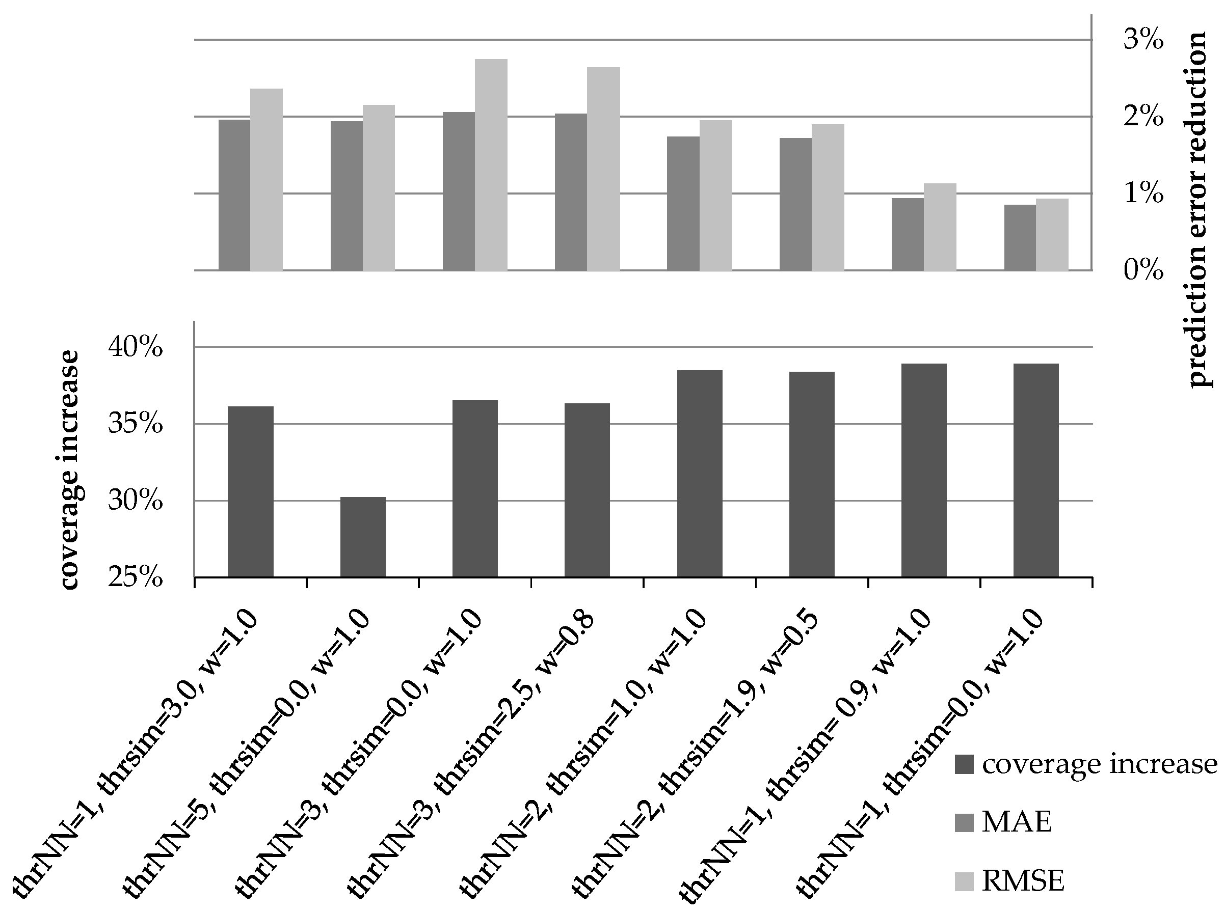
The goal of the first experiment is to determine the optimal values for the parameters thr_NN, thr_sim, and w_dr, used in the CF_DR algorithm. In order to find the optimal setting for these parameters, we explored different combinations of values for them. In total, more than 30 candidate setting combinations were examined. For conciseness, our presentation is confined to the most indicative settings. For each of the parameter combinations, we present the coverage increase and the improvement of the rating prediction accuracy that were achieved (expressed as reduction to the MAE and RMSE metrics). The results were found to be relatively consistent across the seven datasets tested (for the majority of tests, the parameter value combinations were ranked in the same order across all datasets). Consequently, in this subsection, only the average values of the respective coverage increase and error metrics for the seven datasets are presented.

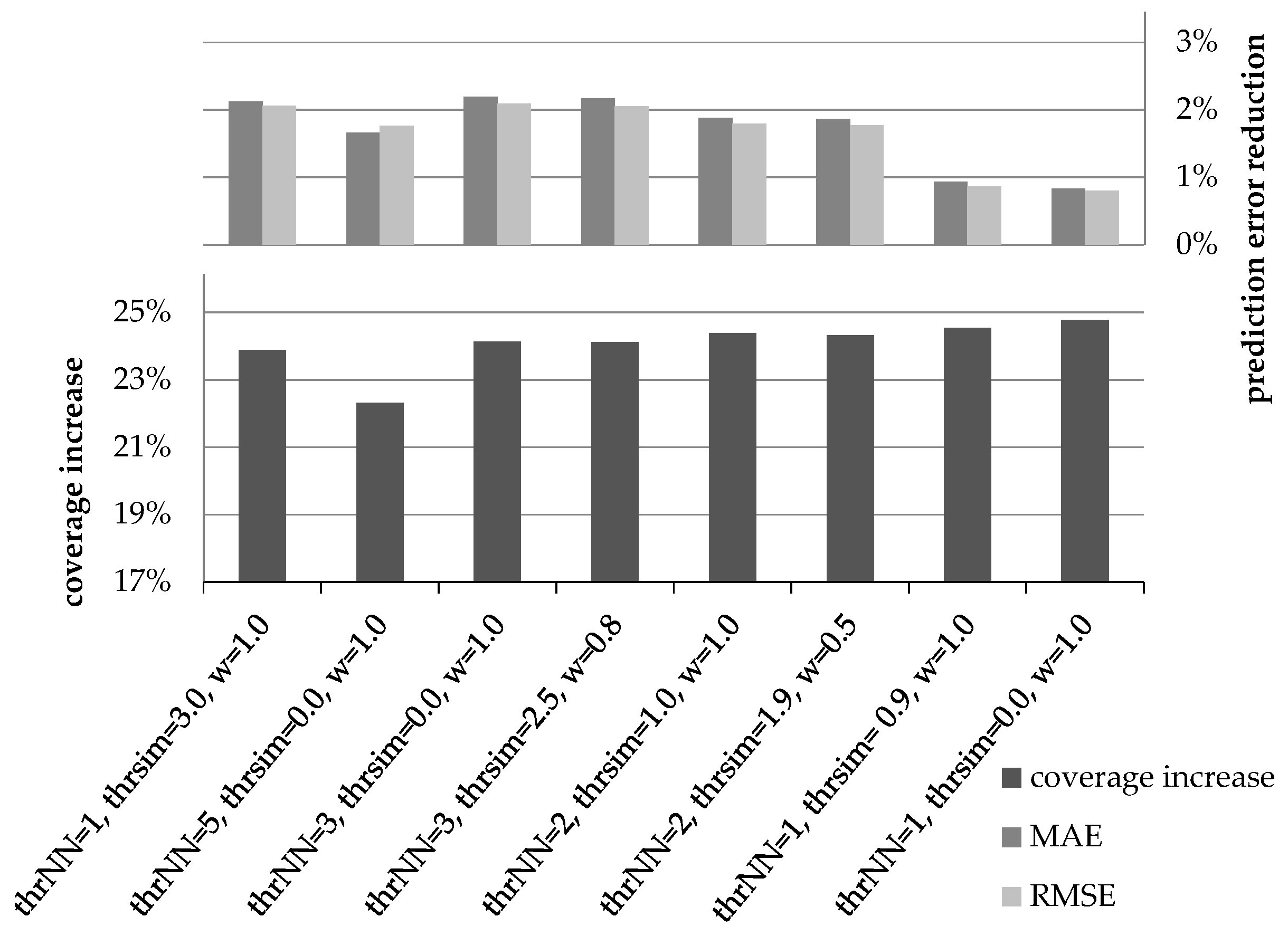
Figure 1 illustrates the coverage increase and the rating prediction error reduction (using both the MAE and the RMSE error metrics) under different settings for parameters thr_NN, thr_sim and w_dr, when similarity is measured using the PCC metric and using the performance of the plain CF algorithm as a baseline. Similarly, Figure 2 depicts the respective measures under the same parameter value combinations, when similarity is measured using the CS metric, again using the performance of the plain CF algorithm as a baseline.

In Figure 1 and Figure 2, we can observe that prediction accuracy improvement does not present maxima and minima under the same parameter combinations. Hence, to determine the best choice regarding the optimal setting of parameters, we synthesize the coverage and accuracy metrics into a single score by computing their harmonic mean (HM). This is analogous to the combination of the precision and recall measures into the F1-measure in the information retrieval domain [55]. Notably, the HM is also used in other RS research works for synthesising coverage and error metrics, e.g., [50]. More specifically, the HM is given by the following formula:

$$\mathrm{HM}\left(\mathrm{s}\right)=2\ast \frac{normCovInc\left(s\right)\times normAccInc\left(s\right)}{normCovInc\left(s\right)+normAccInc\left(s\right)}$$

(6)

where the normalized value for the coverage increase of the setting s, denoted as normCovInc(s), is obtained using the standard normalization formula [55]:

$$normCovInc(s)=\frac{\begin{array}{c}\mathrm{cov}erage\_incr(s)-\min (\mathrm{coverage}\_\mathrm{incr}(\mathrm{s}\left)\right)\\ \hspace{1em}\hspace{1em}\hspace{1em}\hspace{1em}\hspace{1em}\hspace{1em}\hspace{1em}s\in allsettingscombinations\end{array}}{\begin{array}{c}\max (\mathrm{coverage}\_\mathrm{incr}(\mathrm{s}\left)\right)\hspace{1em}-\hspace{1em}\min (\mathrm{coverage}\_\mathrm{incr}(\mathrm{s}\left)\right)\\ s\in allsettingscombinations\hspace{1em}\hspace{1em}s\in allsettingscombinations\end{array}}$$

(7)

Similarly, the value for normalized accuracy according to the MAE error metric is obtained using the same normalization formula:

$$normAcc(s)=\frac{\begin{array}{l}MAE\_reduction(s)-\min (MAE\_reduction\left(\mathrm{s}\right))\\ \hspace{1em}\hspace{1em}\hspace{1em}\hspace{1em}\hspace{1em}\hspace{1em}\hspace{1em}s\in allsettingscombinations\end{array}}{\begin{array}{c}\max (AE\_reduction\left(\mathrm{s}\right))\hspace{1em}\hspace{1em}-\hspace{1em}\hspace{1em}\min (MAE\_reduction\left(\mathrm{s}\right))\\ s\in allsettingscombinations\hspace{1em}\hspace{1em}s\in allsettingscombinations\end{array}}$$

(8)

An analogous formula is employed to obtain the value for normalized accuracy according to the RMSE error metric.

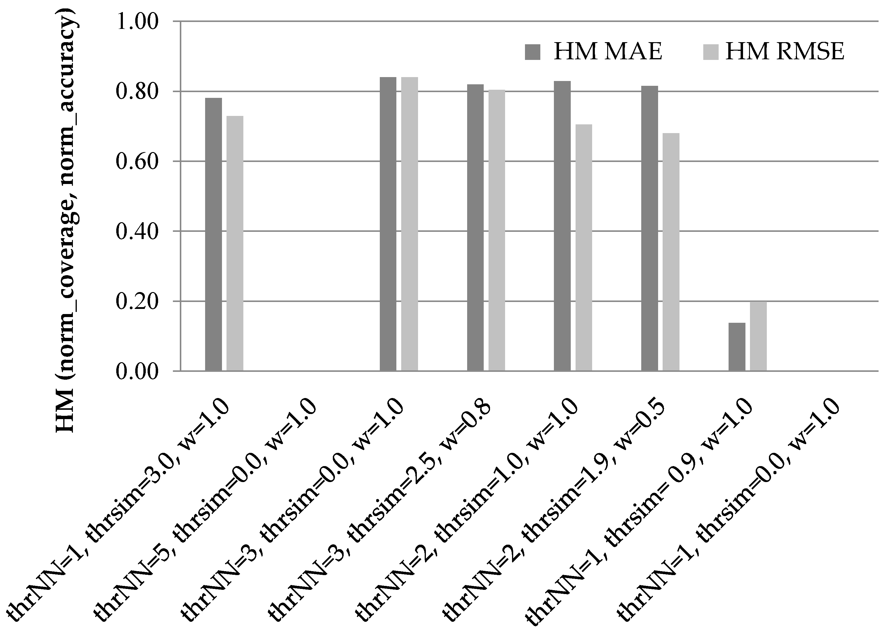
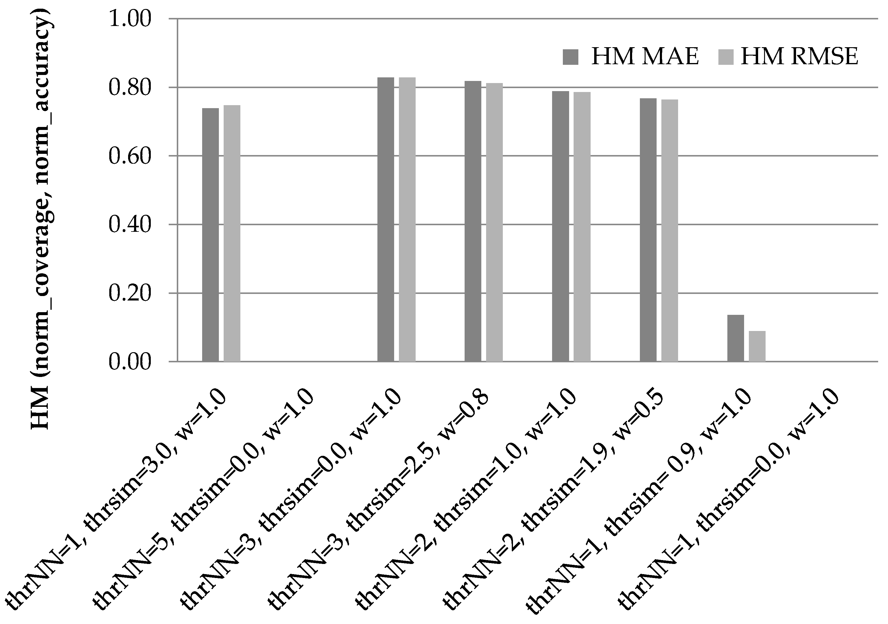
Figure 3 illustrates the results of the HM of the normalized coverage and accuracy increase measures for the candidate settings presented above, when using the PCC as the similarity metric.

In Figure 3, we can observe that the third setting ({thr_NN = 3, thr_sim = 0.0, w_dr = 1.0}) is the best performer across both error metrics, with its harmonic mean being equal to 0.84 under both error metrics. The fourth setting ({thr_NN = 3, thr_sim = 2.5, w_dr = 0.8}) is the runner up, scoring an HM equal to 0.82 under the MAE error metric and 0.80 under the RMSE error metric.

Similarly, Figure 4 illustrates the results of the HM of the normalized coverage and accuracy increase measures for the eight candidate settings, when using the CS as the similarity metric. Again, the performance of the plain CF algorithm is used as a baseline.

In Figure 4, we can observe that again the third setting ({thr_NN = 3, thr_sim = 0.0, w_dr = 1.0}) attains the highest harmonic means under both error metrics (0.83 under both the MAE and RMSE), closely followed by the fourth setting (0.82 under the MAE and 0.81 under the RMSE). The fifth setting ({thr_NN = 2, thr_sim = 1.0, w_dr = 1.0}) follows, with its HM under the MAE being 0.81 and its HM under the RMSE being 0.80.

Taking into account that the third setting ({thr_NN = 3, thr_sim = 0.0, w_dr = 1.0}) achieves the best performance under both similarity metrics and under both error metrics, for the rest of this paper we adopt this setting for all experiments. This practically means that (a) any prediction with at least 3 NNs taking part in its formulation is considered robust and hence produces a DR and (b) the importance of DRs in the prediction formulation process is equal to that of an explicitly entered (real) user rating. This aspect is also exploited for optimization purposes, since no additional information needs to be entered to the user-rating matrix in order to discriminate between real ratings and DRs.

In the next subsection, we present the results obtained in the experiments in more detail, per individual dataset. As noted above, the CF_DR algorithm parameters were set to the values proven to be optimal (i.e., {thr_NN = 3, thr_sim = 0.0, w_dr = 1.0}).

4.2. Performance Evaluation

Following the identification of the optimal parameter values for the operation of the CF_DR algorithm, we evaluated the performance of the algorithm in terms of dataset density increase, prediction coverage increase, and prediction accuracy improvement using the seven datasets listed in Table 4.

4.2.1. Density Increase

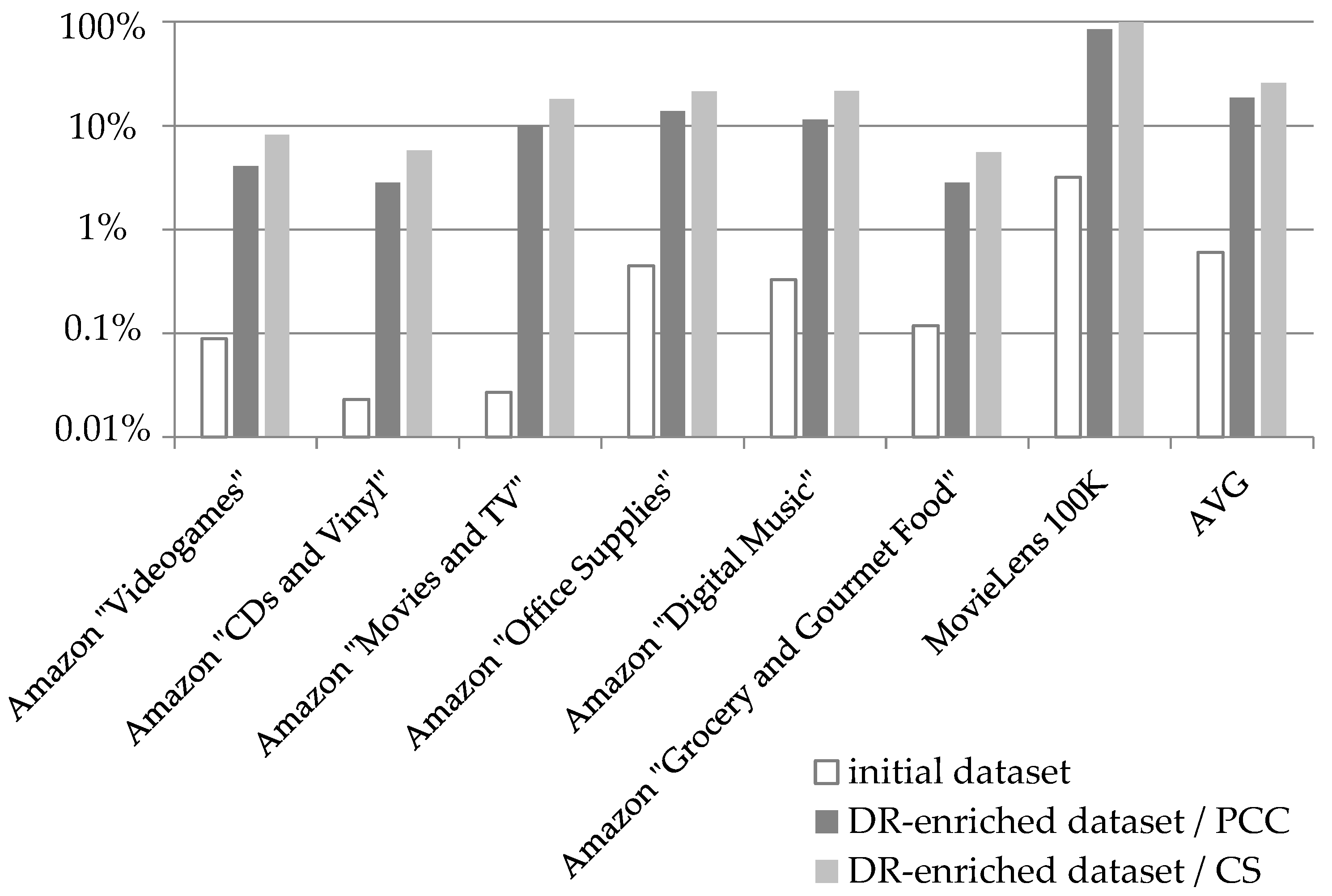
Figure 5 illustrates the densities of the seven datasets listed in Table 4: (a) in their initial form and (b) after the enrichment with the DRs produced by the CF_DR algorithm’s preprocessing step. Note that a base-10 logarithmic scale is used for the Y axis.

Under the PCC similarity metric, the incorporation of the DRs achieves an increase of the average density from 0.6% that the initial datasets averaged, to 18.54%. On the individual dataset level, the density increase achieved by the proposed algorithm ranges from 24 times (initial dataset density: 0.118%; density of DR-enriched dataset: 2.834%), for the Amazon “Amazon Grocery and Gourmet Food” dataset, to 369 times for the Amazon “Movies and TV” dataset (initial dataset density: 0.027%; density of DR-enriched dataset: 9.953%). Furthermore, we can clearly notice that, after the application of the CF_DR algorithm preprocessing step, all the datasets, even the more sparse ones (such as the Amazon “CDs and Vinyl”, having an initial density of 0.023%) exceed the density threshold of 1% set by [56], beyond which a dataset D is considered to be dense.

Correspondingly, under the CS as the similarity metric, again, the incorporation of DRs increases the average density from 0.6% that the initial datasets averaged, to 25.77%. On the individual dataset level, the density increase achieved by the proposed algorithm ranges from 31 times for the MovieLens “100 K” dataset (initial dataset density: 3.17%; density of DR-enriched dataset: 99.7%), to 671 times for the Amazon “Movies and TV” dataset (initial dataset density: 0.027%; density of DR-enriched dataset: 18.12%).

4.2.2. Prediction Coverage Increase

In this subsection, we present the detailed results on the performance evaluation of the algorithm in terms of rating prediction coverage, using the seven datasets listed in Table 4. In this experiment, the performance of the plain CF algorithm is used as a yardstick. Besides obtaining absolute metrics on coverage improvement by the CF_DR algorithm presented in this paper, we perform a detailed comparison between its performance and the performance of the following algorithms:

• The CF_VNN algorithm [27], where artificial user profiles (virtual near neighbours—VNNs) are created by combining pairs of real users which are NNs of high similarity. The CF_VNN algorithm was configured to use the optimal parameters for its operation reported in [27], i.e., Th(sim) = 1.0 and Th(cr) = 1. For more details on the parameters, the interested reader is referred to [27].
• The CF_FOAF algorithm [29], where the transitivity of the NN relationship is explored, and two users can be considered as NNs with each other if they are NNs to a third user. The CF_FOAF algorithm was configured to use the optimal parameters for its operation reported in [29], i.e., Th(sim, src) = 0, Th(sim, targ) = 0, Th(sim, endpoints) = 0, Th(cr, src) = 1, Th(cr, targ) = 1, and Th(cr, comb) = 2. For more details on the parameters, the interested reader is referred to [29].

Both the aforementioned algorithms (a) are state-of-the-art (the CF_VNN algorithm [27] was presented in 2019, while the CF_FOAF algorithm was presented in 2020) algorithms targeting primarily to increase the CF rating prediction coverage and also to alleviate the “grey sheep” problem, (b) achieve considerable improvement in coverage while additionally attaining slight improvement on rating prediction accuracy, and (c) necessitate no supplementary data, such as user relationships obtained from social networks, item categories, etc.

The rationale behind the choice of the CF_VNN and CF_FOAF algorithms, for the performance comparison, is that among all CF algorithms targeting coverage increase without necessitating additional data, the first algorithm is proven to be better at rating prediction accuracy, while the second one achieves higher rating prediction coverage increments. Therefore, by comparing the proposed algorithm with both the CF_VNN and CF_FOAF algorithms, we obtain a holistic view of the algorithm performance, covering both rating prediction aspects (coverage and accuracy).

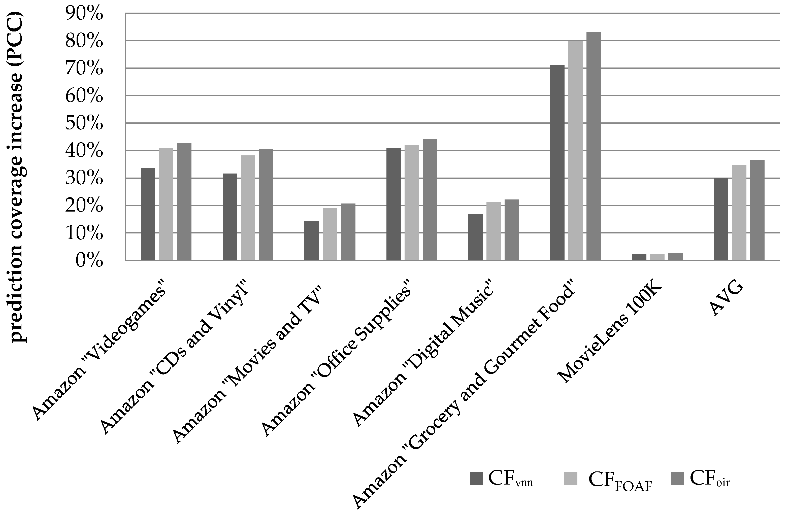
Figure 6 illustrates the results obtained regarding the prediction coverage increase, when the metric used to quantify similarity between users is the PCC.

We can observe that the CF_DR algorithm, presented in this paper, successfully increases the average coverage across all datasets by 36.52% against the baseline (the coverage increment is calculated as $\frac{coverage\left(DR-enricheddataset\right)-coverage\left(baseline\right)}{coverage\left(baseline\right)}$). On the individual dataset level, the coverage improvement ranges from 2.61%, for the MovieLens 100 K dataset, to 83.1%, for the Amazon “Grocery and Gourmet Food” dataset. Notably, the MovieLens 100 K is a dense dataset (its density is equal to 3.17%), consequently exhibiting very high coverage in its initial form (approximately equal to 94%), hence the coverage improvement margin is limited.

The CF_FOAF algorithm, introduced in [29], achieved an average coverage increase of 34.7%, while the CF_VNN algorithm [27] achieved an average coverage increase of 30.1%.

On the individual dataset level, the relative performance edge of the proposed algorithm against the CF_FOAF algorithm, which was found to achieve higher prediction coverage than the CF_VNN algorithm, ranges from 4.1%, for the Amazon “Grocery and Gourmet Food” dataset, to 8.1%, for the Amazon “Movies & TV” dataset, for the sparse (Amazon) datasets that were considered. The average performance edge, across all the sparse datasets, of the proposed algorithm against the CF_FOAF algorithm was measured at 5.44%, while the respective edge against the CF_VNN algorithm was measured at 25.9%.

Regarding the dense dataset “MovieLens 100 K”, the proposed algorithm was found to surpass the performance of the CF_VNN algorithm by a margin of 0.47% in absolute figures, while, in terms of relative improvement, the edge of the proposed algorithm is quantified to 22%.

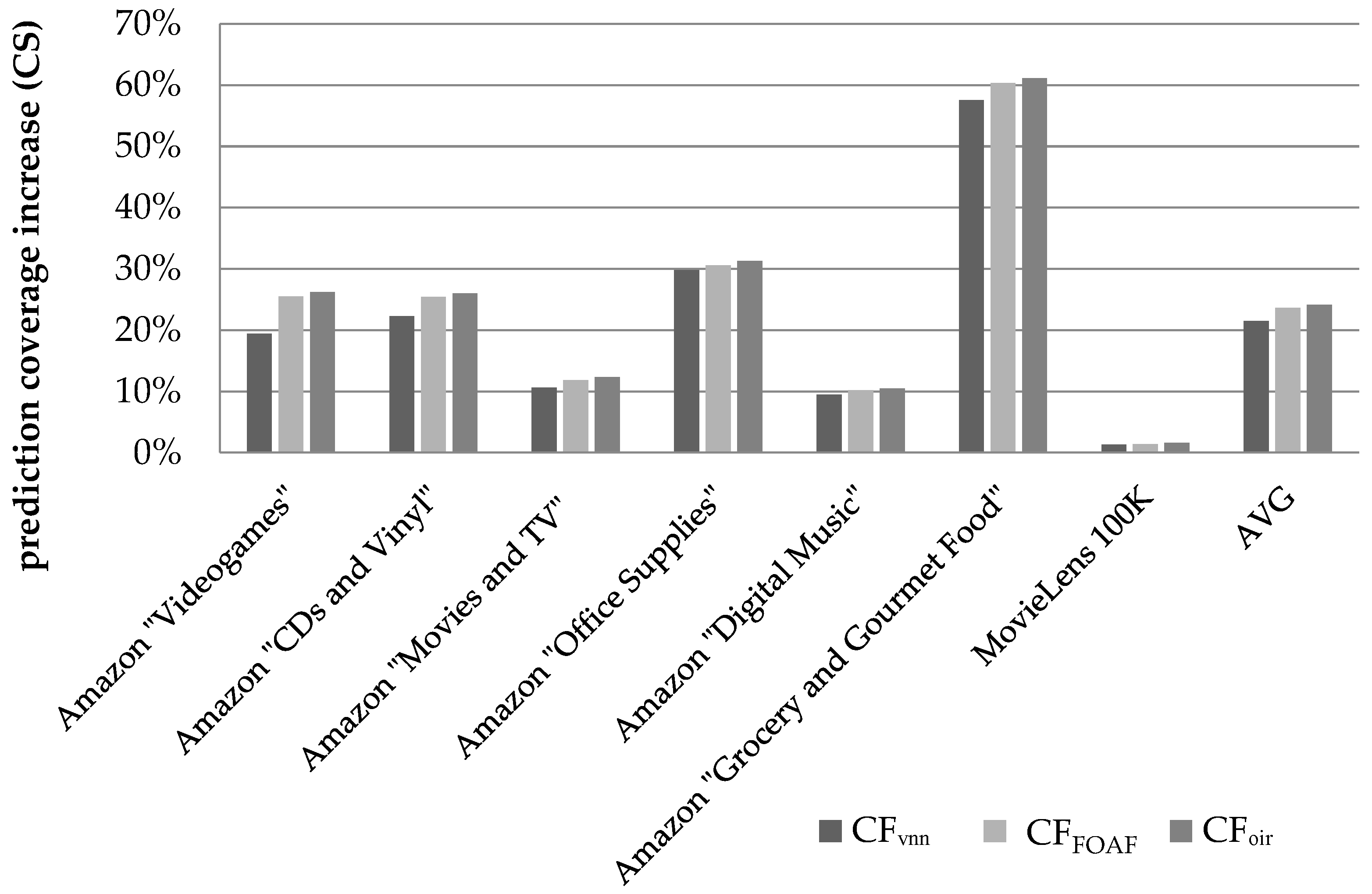
Figure 7 illustrates the respective coverage increase results when CS is used to quantify similarity between users.

We can observe that the CF_DR algorithm, presented in this paper, achieves an increase of the average coverage across all datasets by 24.13% against the baseline. On the individual dataset level, the coverage improvement ranges from 1.59%, for the MovieLens 100 K dataset, to 61.12%, for the Amazon “Grocery and Gourmet Food” dataset. Again, the smallest coverage increase is achieved in the case of the MovieLens 100 K, which, due to its high density and the corresponding high initial coverage, offers little coverage improvement potential.

On the individual dataset level, the relative performance edge of the proposed algorithm against the CF_FOAF algorithm, which was again found to achieve higher prediction coverage than the CF_VNN algorithm, ranges from 1.3%, for the Amazon “Grocery and Gourmet Food” dataset, to 4.4%, for the Amazon “Movies and TV” dataset. The average performance edge, across all the sparse datasets, of the proposed algorithm against the CF_FOAF algorithm was measured at 2.6%, while the respective edge against the CF_VNN algorithm was measured at 14.8%.

Overall, under the CS similarity metric, coverage improvement is lower, when compared to that observed under the PCC similarity metric. This is due to the fact that, under the CS metric, the baseline algorithm (plain CF) exhibits higher coverage (78.5% vs. 60.4% under the PCC), hence the margin for improvement is narrower.

Regarding the dense dataset “MovieLens 100 K”, the proposed algorithm was found to surpass the performance of the CF_FOAF algorithm by a margin of 0.21% in absolute figures, while, in terms of relative improvement, the edge of the proposed algorithm is quantified to 15.2%.

4.2.3. Prediction Accuracy Increase

In this subsection, we present detailed results on the algorithm performance evaluation in terms of rating prediction error reduction, where the error is measured using the MAE and the RMSE metrics, for the same seven datasets. As before, besides obtaining absolute metrics regarding the prediction accuracy achieved by the CF_DR algorithm, we also compare its performance to the performance of the CF_VNN algorithm introduced in [27] and the CF_FOAF algorithm introduced in [29].

Figure 8 illustrates the results obtained regarding the prediction accuracy, in terms of the MAE, when the metric used to quantify similarity between users is the PCC. The considerable differences observed for the values of the MAE metric between the MovieLens dataset on the one hand and the Amazon datasets on the other is that, in the former dataset, the ratings range from 0 to 9, whereas in the Amazon datasets, ratings range from 1 to 5.

We can observe that the CF_DR algorithm, presented in this paper, achieves an average prediction MAE reduction equal to 2.06% (in absolute terms 0.877 versus 0.895, the plain CF achieves), exceeding the performance of the CF_VNN algorithm [27] (which is measured at 1.42%) by 0.64% in absolute figures, or 45.1% as a relative improvement. When compared with the CF_FOAF algorithm [29], the CF_DR algorithm outperforms CF_FOAF (whose MAE reduction was measured at 1.17%) by a margin of 76.3%.

On the individual dataset level, the performance edge of the proposed algorithm against the CF_VNN algorithm (which achieves a higher MAE reduction than the CF_FOAF algorithm), ranges from 25.9% (for the Amazon “Digital Music” dataset) to 84.4% (for the Amazon “Videogames” dataset).

Similarly, Figure 9 illustrates the results obtained regarding the prediction accuracy increase, in terms of the MAE, when the CS metric is used to quantify similarity between users.

In Figure 9, we notice that the CF_DR algorithm, presented in this paper, achieves an average prediction MAE reduction equal to 2.19% (in absolute terms 0.814 versus 0.832, the plain CF achieves), exceeding the performance of the CF_VNN algorithm [27] (which is measured at 1.65%) by 0.54% in absolute figures, or 32.1% as a relative improvement. The CF_DR algorithm also surpasses the performance of the CF_FOAF algorithm [29] (which is measured at 1.55%) by 41.4%.

On the individual dataset level, the performance edge of the proposed algorithm against the CF_VNN algorithm (which achieves higher MAE reduction than the CF_FOAF algorithm), ranges from 8.12% (for the Amazon “Digital Music” dataset) to 79.7% (for the Amazon “Office Supplies” dataset).

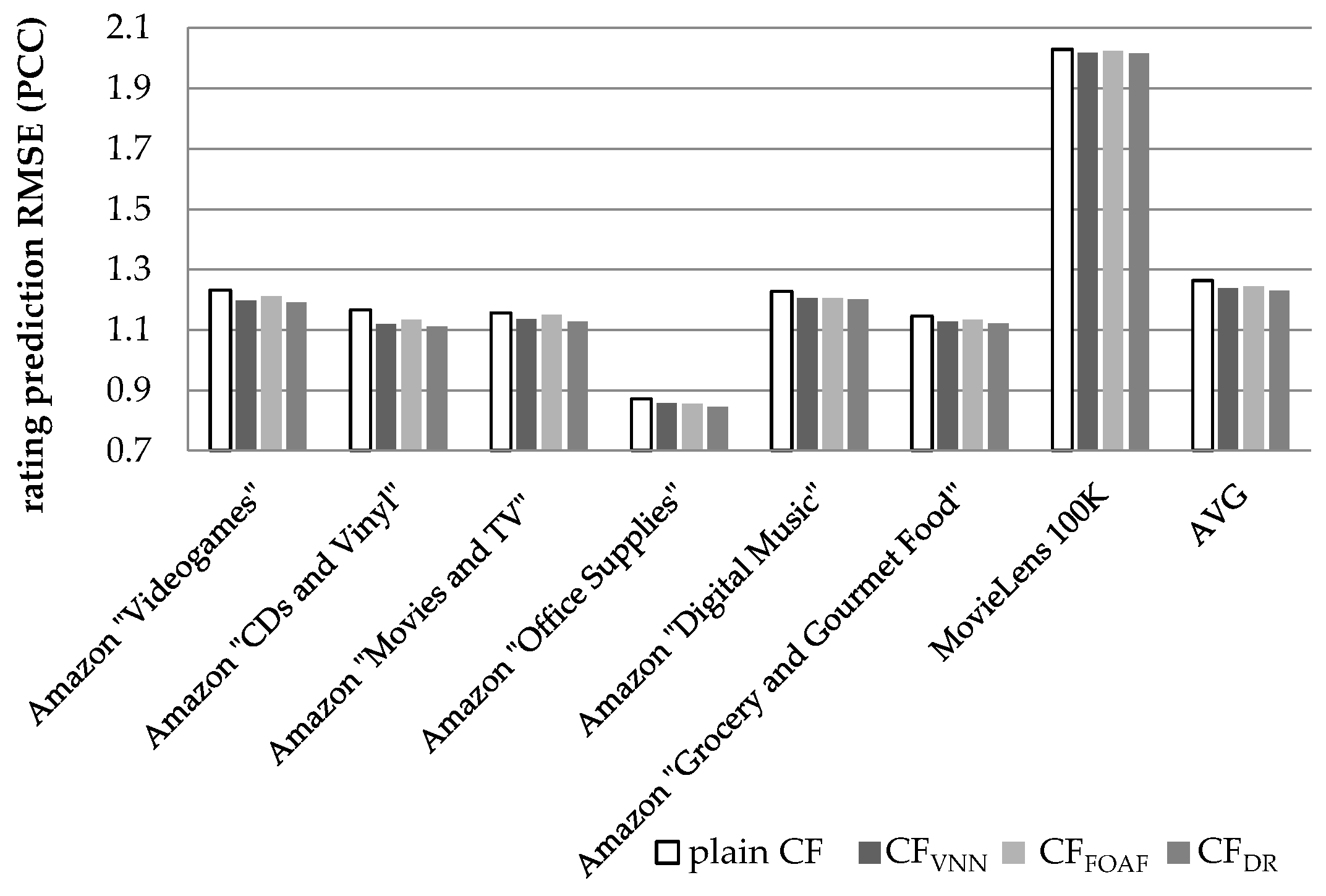
Figure 10 illustrates the results obtained regarding the prediction accuracy increase, in terms of the RMSE, when the PCC was used to quantify similarity between users. In Figure 10, we can notice that the CF_DR algorithm, presented in this paper, achieves an average prediction RMSE reduction equal to 2.75% (in absolute terms 1.229 versus 1.264, the plain CF achieves), exceeding the performance of the CF_VNN algorithm [27] (which is measured at 2.09%) by 0.66% in absolute figures, or 31.5% as a relative improvement. In comparison to the CF_FOAF algorithm [29], the CF_DR algorithm surpasses CF_FOAF (measured at 1.46%) by 88%. Similarly to the case of the MAE, listed above, the considerable differences observed for the values of the MAE metric between the MovieLens dataset on the one hand and the Amazon datasets on the other is that in the MovieLens dataset the ratings range from 0 to 9, whereas in the Amazon datasets ratings range from 1 to 5.

On the individual dataset level, the performance edge of the proposed algorithm against the CF_VNN algorithm, which achieves a higher RMSE reduction than the CF_FOAF algorithm, ranges from 17.5% (for the Amazon “CDs and Vinyl” dataset) to 88.6% (for the Amazon “Office Supplies” dataset).

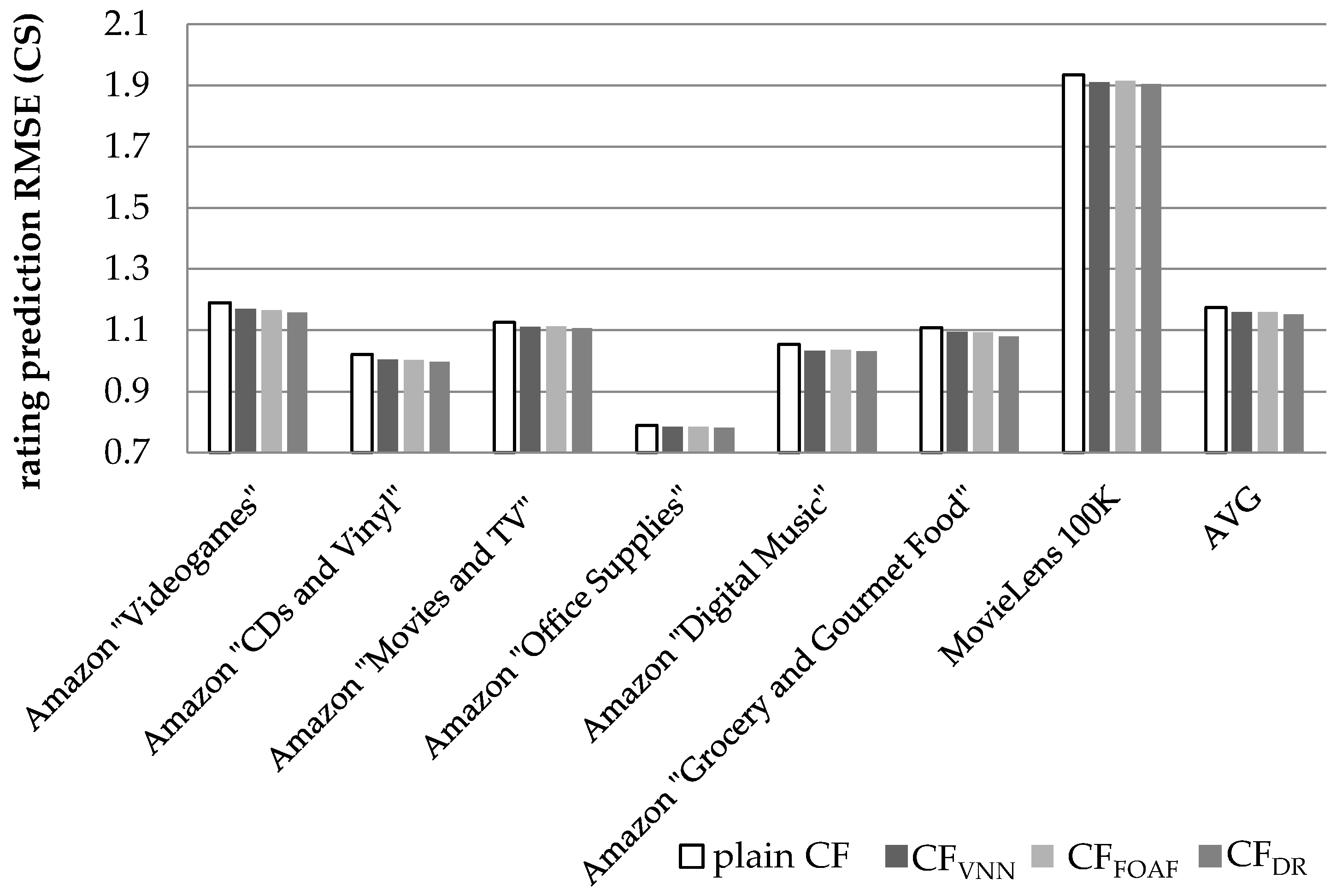
Finally, Figure 11 illustrates the results obtained regarding the prediction accuracy increase, in terms of the RMSE reduction, when the CS metric is used to quantify similarity between users.

In Figure 11, we notice that the CF_DR algorithm, presented in this paper, achieves an average prediction RMSE reduction equal to 2.09% (in absolute terms 1.151 versus 1.176, the plain CF achieves), exceeding the performance of the CF_VNN algorithm [27] (which is measured at 1.48%) by 0.61% in absolute figures or by 41.5% as a relative improvement. The CF_DR algorithm also outperforms the CF_FOAF algorithm [29], whose performance is measured at 1.47%, by 42.2%. On the individual dataset level, the performance edge of the proposed algorithm against the CF_VNN algorithm ranges from 8.95% (for the Amazon “Digital Music” dataset) to 87.5% (for the Amazon “Grocery and Gourmet Food” dataset).

5. Discussion of the Results and Comparison with Other Works

From the experimental evaluation, we can conclude that the CF_DR algorithm, presented in this paper, can successfully increase the density of the CF datasets, regardless of their initial density, since it was successfully applied to both sparse and dense datasets. At the same time, the CF_DR algorithm can achieve both a prediction coverage improvement and a significant prediction error reduction, for both the error metrics tested. In regard to the DR formulation, which is performed within the CF_DR preprocessing step, the optimal setting for considering a prediction as robust (and hence create a DR) is when at least three NNs of a user take part in the prediction formulation. Furthermore, the optimal significance of the DRs was found to be exactly the same with the real (explicit) user ratings.

In the following subsections, we compare the performance of the CF_DR algorithms against other algorithms published in the literature and target the increase of coverage of CF-based algorithms. To provide a fair comparison basis, the algorithms included in the comparison are limited to those which utilize only the user-item rating matrix, without necessitating the availability of additional data, such as social relationships [24,36] or trust [57,58].

In

Table 5. Comparison of CF_DR with algorithms that exploit only the user-item rating matrix for achieving coverage increase.

Algorithm	Evaluation Dataset(s)	Coverage Increase	Accuracy Increase	Comments
HyCov [33]	MovieLens	2.07%	MAE: 0.12%	The CFDR algorithm achieves higher coverage and accuracy improvements as measured using the MAE metric in the same dataset (2.66% and 0.66%, respectively, under a five-fold cross validation performance assessment procedure).
CFVNN [27]	MovieLens & Amazon	avg. for sparse datasets: 30.54% MovieLens: 1.90%	avg. for sparse datasets: MAE: 1.56%; RMSE: 2.33% MovieLens: MAE: 0.46%; RMSE: 0.56%	The CFDR algorithm achieves higher coverage and accuracy improvements both for sparse datasets (avg. coverage increase: 37.17%, avg. MAE improvement: 2.27%; avg. RMSE improvement: 3.04%, under a hide-one performance assessment procedure) and the dense MovieLens dataset (2.54%, 0.61% and 0.67%, respectively, again under a hide-one performance assessment procedure).
CFFOAF [29]	MovieLens & Amazon	avg. for sparse datasets: 35.45% MovieLens: 1.90%	avg. for sparse datasets: MAE: 1.29%; RMSE: 1.67% MovieLens: MAE: 0.36%; RMSE: 0.25%	The CFDR algorithm achieves higher coverage and accuracy improvements both for sparse datasets (avg. coverage increase: 37.17%, avg. MAE improvement: 2.27%; avg. RMSE improvement: 3.04%, under a hide-one performance assessment procedure) and the dense MovieLens dataset (2.54%, 0.61% and 0.67%, respectively, again under a hide-one performance assessment procedure).
ANLF [45]	MovieLens & Jester	None reported; the algorithm is based on matrix factorization, hence a value is predicted for all items for all users	avg. for the MovieLens & Jester datasets: RMSE 0.25% and 0.47%, respectively	CFDR algorithm achieves higher accuracy improvements than ANLF (MovieLens dataset RMSE improvement: 0.71% under a five-fold cross validation performance assessment procedure). Note that, since the ANLF is matrix factorization based, a prediction is always formulated for every empty cell in the user-item rating matrix, with predictions involving users or items having very few ratings degenerating to a dataset-dependent constant value [40]. Despite this particularity, accuracy precisions are comparable because they are always computed considering solely known ratings, because only for these ratings the ground truth is known.

, we can observe that the CF_DR algorithm achieves higher coverage increase than all other state-of-the-art algorithms, both for the cases of sparse and dense datasets. This is also true for the rating prediction accuracy improvement. More specifically, in sparse datasets, the CF_DR algorithm outperforms other algorithms in the prediction coverage by a margin ranging from 1.7% to 6.6% in absolute numbers (or 4.9% to 21.7% as a relative increase), observed for the CF_FOAF [29] and CF_VNN [27] algorithms, respectively. The corresponding accuracy improvement, as quantified by the MAE metric, varies from 0.71% to 0.98% in absolute numbers (or 45.5% to 80% as a relative increase), observed for the CF_VNN [27] and CF_FOAF [29] algorithms, respectively. It is worth noting that the papers cited in Table 5 employ different techniques to quantify coverage increase and rating prediction accuracy: [33] and [45] use a five-fold cross-validation, while [27] and [29] employ the hide-one technique. For comparison fairness purposes, we ran additional experiments to compute the coverage increase and the error metrics using the five-fold cross-validation and the hide-one techniques, and when comparing the CF_DR with another algorithm, we used the results obtained using the same technique employed in the original algorithm publication. In all additional experiments, the CF_DR hyperparameters were set to the best performing composition, i.e., {thr_NN = 3, thr_sim = 0.0, w_dr = 1.0}.

In dense datasets, the CF_DR algorithm outperforms other algorithms in coverage increase by a margin ranging from 0.59% to 0.64% in absolute numbers (or 28.5% to 33.7% as a relative increase), as observed for the HyCov [33] and CF_FOAF [29] algorithms, respectively. The corresponding accuracy improvement, as quantified by the MAE metric, varies from 0.15% to 0.54% in absolute numbers (or 32.6% to 450% as a relative increase), observed for the CF_VNN [27] and the HyCov [33] algorithms, respectively.

6. Conclusions and Future Work

In this paper, we presented the CF_DR algorithm, which is a novel CF algorithm for enhancing the density of sparse CF datasets. The presented algorithm introduced the concept of derived ratings, which are ratings formulated by robust predictions. The experimental results indicated that the optimal setting for considering a prediction as robust (and hence create a derived rating) is when at least three of a user’s NNs take part in the prediction formulation. The experimental results indicated that the optimal significance of the derived ratings, created by the CF_DR algorithm preprocessing step, was the exact same with the real user ratings. Therefore, no other complementary information needs to be stored in the user-item rating DB, except the DRs.

The presented algorithm was experimentally verified using seven datasets. The evaluation results showed that the introduction of the derived ratings achieved to increase the datasets density by 92 times on average, when the PCC similarity metric is applied, and by 172 times on average, when the CS similarity metric is applied, for all the datasets tested. Practically, this density increase effectively transforms the sparse CF datasets to dense, making it possible for other techniques (e.g., matrix factorization [38,39], a technique showing relatively poor prediction accuracy when applied to sparse datasets [40,41]) to be used to further improve prediction accuracy and/or recommendation quality. The proposed algorithm was also applied to a relatively dense dataset (the MovieLens 100 K, whose initial density was 3.17%) and has also been found to successfully increase both its density and coverage further, leading to additional improvement in the rating prediction accuracy. This indicates that the algorithm can be employed across all datasets, regardless of their densities. Hence, a CF system implementation may employ the proposed algorithm, without even examining the properties of the used dataset.

Furthermore, the proposed algorithm achieved to increase CF rating prediction coverage by 36.5% on average when the PCC similarity metric was applied and by 24.1% on average when the CS similarity metric was applied. In regard to CF rating prediction accuracy, the CF_DR algorithm achieved a MAE reduction of 2.06% and a RMSE reduction of 2.75%, when the PCC metric was applied. The respective average reductions for the CS similarity metric were 2.19% and 2.09%.

Moreover, the CF_DR algorithm, was also compared with (a) the CF_VNN algorithm introduced in [27], where artificial user profiles (Virtual Near Neighbours—VNNs) are created by merging pairs of NN profiles corresponding to real users, and (b) the CF_FOAF algorithm introduced in [29], where two users can be considered as NNs with each other if they are NNs to a third user. Both of these algorithms contribute to the “grey sheep” problem alleviation. The CF_DR algorithm was found to consistently outperform both the CF_VNN and the CF_FOAF algorithms in all tested datasets and under both similarity metrics, for both rating prediction accuracy and coverage. A comparison was also made against state-of-the-art algorithms aiming to increase rating prediction coverage utilizing only the user–item rating matrix and has been shown to outperform all of them by a considerable performance margin.

Regarding our future work, we plan to examine the proposed algorithm using additional correlation metrics, such as the Spearman coefficient, the Euclidian distance, and the Manhattan distance [59]. Adaptation of the proposed approach, so that it can be directly combined with MF techniques [38,39], and exploit the benefits of merging estimators [11,12,13] will also be considered. Finally, the adaptation of the CF_DR algorithm to take into account additional information, such as social network information, item (sub-)categories, and user characteristics and emotions [60,61,62,63], will be also investigated.