1. Introduction
Fast data streams are applied by various applications, such as multimedia, communication and sensory devices. The applications demand higher quality data to perform more accurate analysis of information in a data stream. Therefore, the amount of data is getting larger and the communication speed is also getting higher. Additionally, the current trend of data type tends to a continuous stream. It never allows any processing chance with stalling for a temporal buffering. For example, medical applications, like MRI (Magnetic Resonance Imaging) in its analysis and image inspection in industrial factory, must communicate fast, analyze the data stream, and compactly store the original pixel data stream to storage device.
The equipment needs to communicate with each other at high data rate to address the communication problem against the increasing data amount. For example, peripheral buses are now communicating at hundreds of GBytes/sec. However, this causes another problem, which is a difficulty to implement the very fast communication bus. To overcome the challenge that is posed by the requirement of high data rate, we focus on decreasing the transferred data by using lossless data compression.
Since 1950s, the lossless data compression methods have been widely used to encode data to the smaller size and decode it to the original. The arithmetic coding [
1] is one of the traditional methods for compressing data, which applies Shannon’s information entropy. The Huffman coding [
2] is very well known. The coding method assigns the shorter bit pattern to the more frequent data pattern. Subsequently, it encodes the original data to the smaller sized codes. Another is a method that is based on a look-up table. The LZW (Lempel-Ziv-Welch) [
3,
4] is the typical algorithm, which applies widely to such ZIP compression software. It stores patterns appeared in data to a look-up table. The compressor encodes the patterns to indices of the table by matching a part of data to an entry in the table. If the indices consist of shorter bits than the original data patterns, it can compress the original data. Complete implementations of these methods are inevitably based on software, because it needs to make chunks from data stream to analyze frequency in the look-up table by buffering the chunks to a memory. The analysis of chunk needs faster memory performance to increase the bandwidth of compressing process. The applications that process extremely fast data stream demand high performance implementation of lossless data compression on hardware. However, the buffering problem causes difficulty in implementing it.
On the other hand, the recent research trend of lossless compression focuses on the machine learning approach. For example, L3C [
5] performs lossless compression of image data by using a deep neural network based on the cross-entropy [
6] model. The network organizes a connection among an RNN (Recurrent Neural Network), a quantizer, and a CNN (Convolutional Neural Network). The compression process does not include regressive process. Therefore, it performs fast compression by CPU/GPU. Additionally, it is available to parallelize the network and speedup the compression. However, it is dedicated to image data because the cross-entropy includes a minimization between the exact and the estimated probabilities. This means it is not a true lossless, but a visual one. Moreover, when we consider the RNN/CNN, those need very large amount of hardware resources and high speed memory to acquire good performance, and do not treat data stream. Thus, we need a novel lossless data compression algorithm for fast data stream, which is suitable for a compact hardware implementation without any memory access.
This paper proposes a novel lossless data compression algorithm that completely supports streaming data, called Adaptive Stream-based Entropy (ASE) coding. It compresses continuous streaming data using a look-up table without stalling/buffering by assigning the fewest bits to the compressed data. The bits are generated from an adaptive and an instantaneous entropy calculation. The mechanism is suitable for hardware implementation.
The main contributions of research results described in this paper are the following:
We found that the number of occupied entries of a look-up table used in a stream-based data compression strongly relates to data entropy of a streaming data. Using the characteristic. we have developed a novel algorithm, called ASE coding. It compresses a data stream by applying instantaneous entropy that is calculated from the number of occupied entries in its look-up table. We have also found that this algorithm is suitable for hardware implementation.
We have developed a unique table management for ASE coding. It effectively keeps the table entries in the lower part of the look-up table. We also developed an optimization technique, called entropy culling, which performs dynamic reduction of occupied entries in the table.
In order to reduce hardware resources and speedup the implementation, we introduced near neighbor entry exchange, which limits entry exchange to a near place in the look-up table. It contributes to implementing the mechanism on a compact hardware by reducing the size of multiplexer to select the entry.
The rest of the paper is organized, as follows. The next section describes the backgrounds and the definitions of this research. In
Section 3, we will explain the detailed algorithm of ASE coding. In
Section 4, applying ASE coding, we will perform evaluations for compression performance using benchmarks and also report experimental hardware performance implemented on FPGA. Finally, we will conclude this paper.
2. Backgrounds and Definitions
Continuous data flow that does not have the definition of the length is called streaming data in this paper. The streaming data can be generated from, for example, sensory devices, such as measuring atmosphere, human motion, and video/audio streams. The recent fast sensors, such as CMOS image sensors, generate data stream by the clock speed of GHz order, such as MIPI (Mobile Industry Processor Interface). However, software-based implementation of any algorithm can not process stably a high speed data stream, especially by embedded processor due to its limited performance. When we consider data compression, the processor needs to calculate frequency (i.e., counting data patterns). However, it needs not only high processing speed but also high memory I/O performance. Therefore, we need to consider its hardware acceleration to maintain such compression/decompression operations in a fixed time.
The frequency is calculated, depending on information entropy. The information entropy
S is calculated by the following well-known equation, where
is the probability of the data pattern;
For example, the entropy S of an ASCII string “ABDAABBBBD”, which is 80 bits, can be calculated like this: ’A’, ’B’, and ’D’ appear three, five, and two times, respectively. Therefore, where , , and , S becomes about 1.48. The string can be expressed with two bit codes resulted by the ceil function of S. If ’A’, ’B’, and ’C’ are assigned to the code bits ’00’, ’01’, and ’10’, the data can be compressed to ”00011000000101010110”, that is 20 bits. Therefore, the compression ratio is .
The Huffman coding [
2] improved the coding mechanism to assign the shortest code to the most frequent data pattern by using a binary tree where each node has 1 in the left and 0 in the right of the parent node. The right node of the root is the most frequent pattern. In the case above, ’A’, ’B’, and ’D’ are assigned to ’01’, ’1’, and ’00’. Thus, the string is compressed to ”011000101111100”, which is 15 bits. This results better compression ratio than the case of the fixed size codes. In these cases, the decoder can decompress the encoded string using the combinations made by pairs of the original and the assigned codes.
Here, let us consider applying the coding mechanisms above to streaming data. As discussed before, streaming data are continuous. It is impossible to obtain the entropy of a streaming data since the data arrive sequentially. To avoid this blocking operation, some compression implementations split the original data to small chunks. Subsequently, these process each chunk one after another. For example, deflate [
7] uses Huffman coding in the latter part of the compression processes. It splits data stream into small chunks, counts the frequency, and assigns codes for every chunk. However, this also needs to buffer the chunk. Therefore, a very fast physical memory is unavoidable at its hardware implementation in order to maintain high speed compression performance. On the other hand, unless making chunks of streaming data, it is potentially impossible to count frequency of data patterns of whole streaming data. If any online processing is available, it is the best method to assign the shortest bit code of the patterns continuously to streaming data as soon as the patterns are inputted to the compressor. Dynamic Huffman coding [
8] is proposed to improve the buffering overhead. It adaptively generates the binary tree with processing every input data symbol. The tree represents the codes that are assigned to the original data symbols as well as the original Huffman coding. The nodes and the height of the tree are dynamically exchanged and adjusted at every input symbol. When we consider to implement it on hardware, the operations are too complex to maintain a constant number of steps for the exchange and adjustment of the tree. Therefore, it does not fit to hardware implementation.
Another concept has been applied to the conventional algorithms, such as the former part of Deflate [
7], Google’s Snappy [
9] and LZ4 [
10]. These are originally LZ-based compression mechanisms that use a look-up table to store frequent patterns. Deflate uses both LZ77 and Huffman coding by making small chunks of input symbols. It works like a stream-based. However, it is not completely stream-based because it needs buffer for the chunk. Snappy and LZ4 improves the processing speed of LZ. However, it skips long pattern comparison when it misses in the look-up table. This promises the high bandwidth by degrading the compression ratio. LZ4 also employs the stream-like method with making chunks of input data. In the conventional compression methods that are based on look-up table, the table length must be variable because the stored patterns can be any length. This is not suitable for hardware implementation, because we can not decide an appropriate size of the table.
The recent advanced researches of lossless data compression focus on the machine learning approach. Those are mainly targeted to image data compression. For example, powerful methods, called PixelRNN [
11] and PixelCNN [
12], predict the distribution of pixels using an RNN and a CNN with masked convolution. These are called visually lossless compression that do not indeed generate the same color data as the original pixels. However, the compression ratio is efficiently high. During the calculations of the networks, those include back propagation calculations. This does not allow them to accept data stream due to blocking it by the heavy calculation. On the other hand, L3C [
5] implements lossless compression by applying the cross entropy model that includes a minimization between the exact and the estimated probabilities. Therefore, it is also the visually lossless compression. It eliminated the back propagation during the RNN/CNN calculations, and then implements fast compression. The compression process can also be parallelized. This brings faster compression by multiple CPUs/GPUs. We can also find similar approaches by neural networks, such as PAQ [
13], DeepZip [
14], and CMIX [
15]. However, this deep neural network approach needs many resources in order to implement the network calculations in hardware, and also high performance memories to speedup the learning phase. Thus, it is unfeasible to implement these methods in a compact hardware that allows for continuously accepting streaming data.
On the other hand, hardware-based approaches, such as nx842 [
16] and LCA-DLT [
17], are proposed. The nx842 is used in POWER processors to compress data stream in the memory bus. It compresses streaming data of memory I/O by encoding symbols using coding templates and pattern tables that maintain parts of frequent symbols. The compression ratio is affected by the memory size for the templates and the patterns. Therefore, it needs a larger memory size to achieve better compression ratio. Finally, LCA-DLT works to process completely streaming data, and it can be implemented in a small hardware resources, such as FPGA. It is implemented on a module that compresses a data pair to a compressed symbol by a fixed sized look-up table. The modules can be cascaded to compress longer data pattern. However, the compressed data size is not variable, i.e., fixed to the symbol size. Therefore, the compression ratio of a module becomes more than 50%. To improve this, it inevitably cascades the modules to improve the compression ratio. This causes hardware resource increase.
This paper proposes a novel coding mechanism, called ASE (Adaptive Stream-based Entropy) coding, which encodes streaming data by assigning adaptive code from instantaneous entropy of streaming data in order to address the drawbacks of the conventional lossless data compression algorithms discussed above. The mechanism is suitable for hardware implementation, which can be implemented with limited resources.
3. ASE Coding
We propose a novel stream-based data compression mechanism that performs real-time entropy coding by assigning the shortest code bits to a symbol that appeared at the moment when the symbol of a streaming data is received by the compressor. It can be implemented easily and compactly on hardware and compresses/decompresses streaming data, which works at every clock cycle. Let us begin to explain the algorithm from its overall organization.
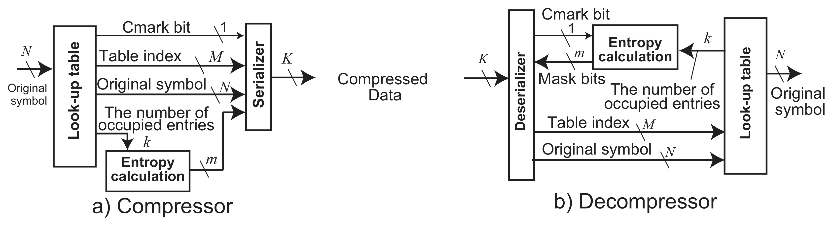
3.1. Organization of Compressor/Decompressor
The compressor and the decompressor of ASE coding are organized, as shown in
Figure 1. The compressor receives every fixed-size data at every clock cycle. Here, we call the
N bit data an original symbol
s. The decompressor decodes its compressed data and outputs the original symbol. Both the compressor and the decompressor consist of three parts: a look-up table, an entropy calculation, and a serializer in the compressor and a deserializer in the decompressor.
The look-up table saves frequent data symbols from the inputted data stream. The table includes one or more entries which width equals to N bits. The compressed data are generated from an index of the table. Contrarily, the decompressor picks up a symbol by using the compressed data as an index of the table. The number of bits of the table index is where E is the total number of the table entries.
The entropy calculation generates a pseudo entropy
m from the number of occupied entries
k in the look-up table, as follows:
Here, m represents the shortest bit length of an instantaneous entropy. It depends on E of the number of entries in the table that maintains the recent frequent patterns. ASE coding tries to minimize m adaptively against streaming data. The serializer shrinks the compressed data to m bit length by removing the most significant bits from a table index (i.e., an index of matched entry in the look-up table). Here, let us describe the compression mechanism formally: to derive a compressed data stream D in K bit wide, , where is a function that associates the matched index of the look-up table. where ⊗ is a function to shrink to m bits. , where is a function that concatenates a compressed symbol a to a compressed data sequence b. For example, in the case when and , the function concatenates to the last of and outputs ’1101100101’ as again. Finally, where is a function that serializes a compressed data sequence a with dividing by b bit(s). For example, if and , m becomes 4. In this case, when the compressed data is ’000101’, it is shrunk to ’0101’. Subsequently, the serializer generates a stream of the compressed data by aligning to K bit(s) of the output interface width. In software implementation, the concatenate function performs buffering to a memory and then passes it to the serialization function. Besides, in hardware implementation, it passes the bit stream of to the serialization function by using a barrel shifter. This allows for the compression operations to perform in a pipeline manner.
When the K bit data have arrived the decompressor, the deserializer receives m from the entropy calculation and extracts the first m bits from its stream of the K bit data. The decompressor applies it to the index of the look-up table. Here, the extracted m bits are extended to M bits by adding 0s in the most significant part. Let us describe the decompression mechanism formally: where is a function that deserializes K bit data slices consists of to a bit stream of b. , where is a function that extracts b bits from a bit stream a. where is a function that extends a compressed symbol a to b bit(s). Subsequently, is used as an index of the look-up table and the original symbol is derived as , where is a function to pick up a content of table entry indexed by . For example, when a little-endian stream “010 011 100 …” of is received by the decompressor, if , ’11010’ is extracted (”010” is merged in the lower part, and ”11” is done in the higher one. However, three ’0’s in the MSB are added to M). When , it is extended to “00011010”. Finally, it is used for an index of the look-up table.
Thus, as symbols are continuously inputted to the compressor, the compressor translates the symbols to the indices of the look-up table as the compressed data. The compressed data is shrunk by the entropy calculation. The serializer outputs it to the interface. The decompressor deserializes and extracts the compressed data using the entropy calculation. The compressed data are used as an index of the look-up table and finally an original symbol is outputted from the decompressor.
3.2. Compression and Decompression Mechanisms
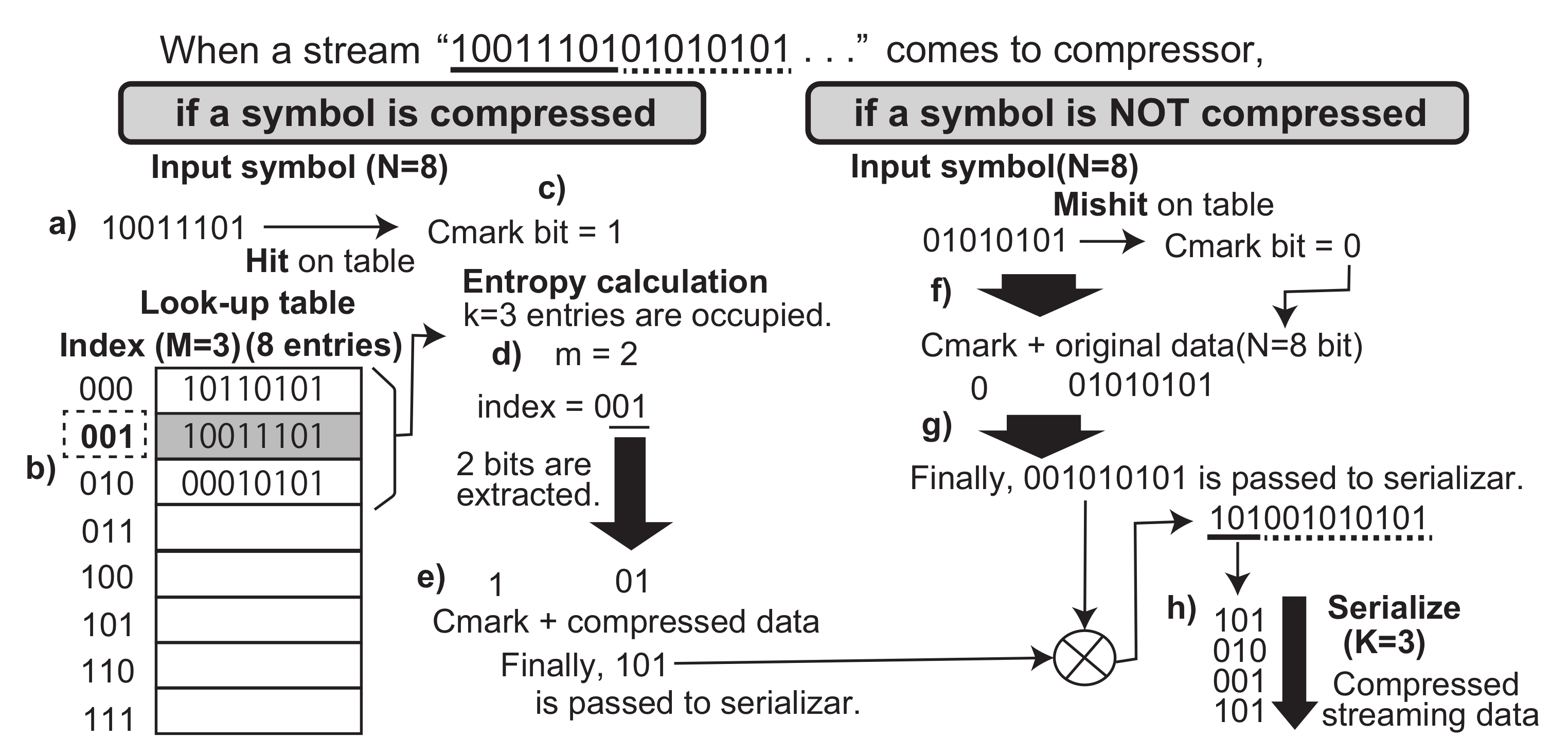
Again, let us focus on the flow how ASE coding compresses and decompresses symbols in a streaming data. Let us begin from the basic operations. When a symbol is received by the compressor, if the symbol is not registered in the look-up table yet (the right side of
Figure 2), the entropy calculation generates
. This indicates that the compressor just outputs the symbol without compression. Finally, the symbol is registered to the look-up table. On the other hand, if the symbol is already registered in the table (the left side of
Figure 2), the entropy calculation generates appropriate
m according to the occupancy of the table. Here, the symbol is shrunk by the entropy and compressed data are generated. Actually, the compressor and the decompressor must treat any
N bit patterns of a symbol. This needs an additional bit to recognize whether an output data is a compressed symbol or an original one. Here, we introduce another
Cmark bit to indicate one of those. We concatenate ’0’ to an original symbol and ’1’ to a compressed data at the most significant bit.
Now, let us extend the formal compression operation with consideration of the Cmark bit, as follows: . . . . Here, the function also outputs the Cmark. The function concatenates also the Cmark bit to the compressed data sequence.
Algorithm 1 summarizes the compression algorithm of ASE coding. Here, the
Initialize() function is invoked to initialize
k, which is the number of occupied entries in the look-up table
T. The table is implemented in an array with
E elements of
Nbit length each. The
ASECompress(
s) is executed to compress a symbol. In the function, the CMark bits is concatenated in the LSB. When the symbol search function
returns
(i.e., the symbol is not registered in the look-up table), the symbol is concatenated with 0 as the CMark bit. Otherwise, the table index
I is shrunk by the
m returned by the
EntropyCalc() function and 1 as the CMark bit is concatenated to the
m bits. The
ASECompress(
s) finally returns
bits as a compressed symbol when the input symbol is missed in the table. Otherwise, it returns
bits. The returned bits are passed to a serializer in order to reform the data stream in
K bit wide. Here, the important point is that the
m is not transferred to the decompressor because the decompressor is able to associate the same
m from the table operation. Let us discuss this after explanation of decompression mechanism. During the table search function
, the look-up table management functions,
ArrangeTable() and
RegisterToTable() are executed. We describe these functions in the next section.
| Algorithm 1 Compression process of ASE coding. |
function Initialize() k = 0 end function
function ASECompress(s) I = (s)) if I == − then 1 CMark = 0 = ( 1) | CMark return else CMark = 1 m = EntropyCalc() = ((I & ((1 ≪m) − 1)) ≪ 1) | CMark return end if end function
function (s) for I:= 0 …k do if T[I] == s then ArrangeTable(s) return I end if end for RegisterToTable(s) return -1 end function
function EntropyCalc() m = return m end function |
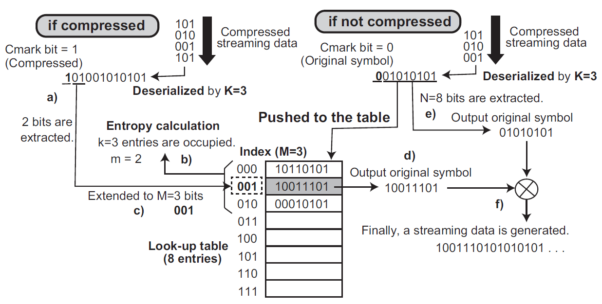
At the decompressor side, when a compressed symbol comes (the left side of
Figure 3), that is, Cmark bit (the most significant bit) is 1, the deserializer refers
m generated by the entropy calculation. Subsequently, it picks up
m bits as a compressed data. The bits are extended to
M bits as an index of the look-up table. Finally, the original symbol is associated from the table, and then is outputted from the decompressor. Besides, if Cmark is 0 (the right side of
Figure 3), the deserializer ignores the entropy calculation and picks up the next
N bits as an original symbol. The symbol is registered to the table and it is outputted from the decompressor.
Regarding the decompression operations with the Cmark bit, the formal expression of the method is extended, as follows: . . . When , is used as an index of the look-up table and the original symbol is derived by . Otherwise, and .
Algorithm 2 shows an implantation example of the decompressor. The pseudo code receives a compressed data stream from the compressor that is shown in Algorithm 1. In the algorithm, we do not show the deserializer. We assume that contiguous bits S are extracted from a compressed data stream reformed by the deserializer at least in () bits. The Initialize() function resets k as well as the compressor. The ASEDecompress() function is executed to decompress a compressed symbol S. Because the CMark bit is concatenated in the LSB of S by the compressor, first, the function extracts the bit and checks if the symbol is compressed or not. If the CMark equals to 1, S is compressed. The m is derived from the entropy calculation and the table index I is extracted as the S is masked by m bits. Then, the original symbol is picked up from I-th element in an array of the look-up table T. Otherwise, an N bit symbol is extracted from S and it is registered to the look-up table. The ArrangeTable() and the RegisterToTable() functions are the same as the ones in the compressor. The timings to be called in both the compressor and the decompressor are also the same. Therefore, the entropy calculation regarding s in the decompressor returns the same m as one regarding the corresponding symbol in the compressor. Therefore, in the compressed data stream, the m is not included in the compressed data stream and it is able to be associated consistently in both compressor and decompressor.
Although we have explained how the compress/decompress operations work, we did not describe how symbols were registered to look-up table in which the
RegisterToTable() and the
ArrangeTable() functions performs. Let us explain it in the next section.
| Algorithm 2 Decompression process of ASE coding. |
function Initialize() k = 0 end function
function ASEDecompress(S) CMark = S & 1 if CMark == 1 then m = EntropyCalc() I = ( 1) & ((1 ) − 1) s = T[I] ArrangeTable(s) else s = S & ((1 ) − 1) RegisterToTable(s) end if return s end function
function EntropyCalc() m = return m end function |
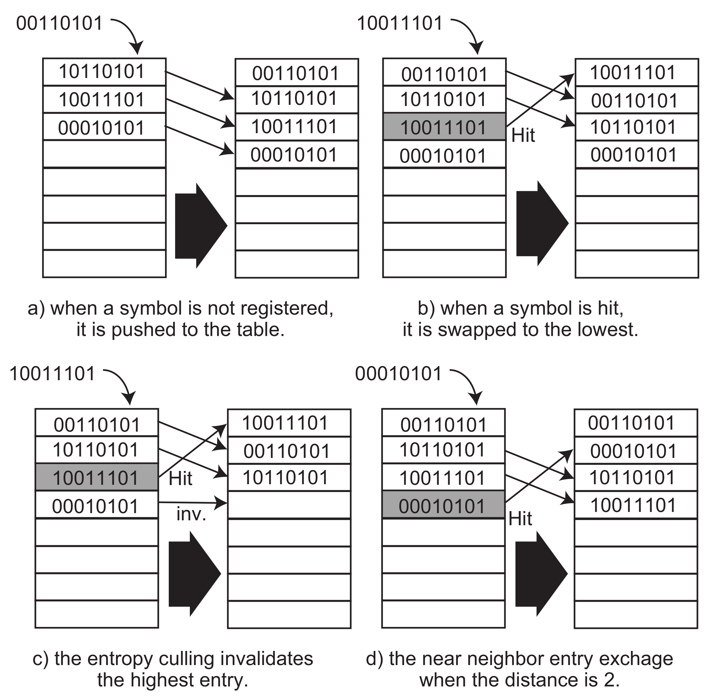
3.3. Look-Up Table Operation
The most important part in the mechanisms of ASE coding is operations of the look-up table performed during the functions
T and
. The look-up table works like a stack. When a symbol arrives, and if it is not registered in the table, the symbol is pushed to the lowest entry of the table, as illustrated in
Figure 4a. If the table is full, the last entry in the table is popped out from the table and discarded. On the other hand, when a symbol is matched to an entry in the table, as depicted in
Figure 4b, the entry is moved to the lowest entry, and then the entries placed from the lowest one are pushed to the higher places as well as the well-known least recently used method.
Algorithm 3 demonstrates the table operation functions. The
RegisterToTable() function executes the table operation depicted in
Figure 4a. It moves all occupied entries of the look-up table
T to the next ones, and then pushes the new symbol entry
s to the lowest entry. It increments
k after pushing
s to the table, while the maximum value of
k is less than
E. Besides, the
ArrangeTable() function executes the table management operations illustrated in
Figure 4b. It moves the hit entry of
s to the lowest one, and pushes the other entries less than the hit one to the next entries. In the Algorithms 1 and 2, the
RegisterToTable() function is called when a symbol
s is missed in the table. Otherwise, the
ArrangeTable() is called. Each function is invoked in both the compressor and the decompressor regarding the corresponding symbol. Therefore, the look-up table
T and also the number of occupied entries
k maintain the same contents among the compressor and the decompressor. Thus, the entropy calculation is able to return the same
m in both sides and the compressor does not need to convey the
m to the decompressor side.
| Algorithm 3 Look-up table management functions of ASE coding. |
functionRegisterToTable(s) for i:= k …0 do if (i + 1) < E then T[i + 1] = T[i] end if end for T[0] = s if (k + 1) < E then k = k + 1 end if end function | functionInitialize() = NUM_CULLING end function
functionEntropyCulling() if > 0 then = − 1 else k = k− 1 = NUM_CULLING end if end function |
| |
functionArrangeTable(s) for i:= 0 …k do if T[i] == s then break end if end for = s for j:= 0 …i− 1 do T[j + 1] = T[j] end for T[0] = EntropyCulling() end function | functionArrangeTableNNEE(s) for i:= 0 …k do if T[i] == s then break end if end for = s = i−d if < 0 then = 0 end if for j:= …i− 1 do T[j + 1] = T[j] end for T[] = EntropyCulling() end function |
However, the table is getting full if the number of symbol patterns increases to more than E. m from the entropy calculation is going to become full bits that equal to , where E is the number of entries in the table. This causes a situation that the compressed data is always M bits plus Cmark bit. To reduce the bits, we apply an optimization function, called Entropy Culling, which reduces the number of occupied entries in the table dynamically during the table operations.
The entropy culling invalidates the highest occupied entry in the table after a number of matches, as illustrated in
Figure 4c. It is managed by a global counter that is decremented by a hit to any table entry. For example, when the counter is set to two, after the second hit, the entropy culling is performed and then the counter is set to two again. This means that the occupied entries are dynamically invalidated at every culling operation. It reduces
and the entropy calculation can generate a smaller
m during the repeated matches in the table. Thus, the compressed data are shrunk to the smaller number of bits adaptively. This mechanism is easily implemented in hardware. For example, let a register with
M bits have the index of the highest occupied entry in the look-up table. Initially, it is reset to 0 (i.e., the lowest entry in the table). Additionally, a counter to count the number of hits in the table mentioned above is prepared. During the stacking operation to register a new symbol to the table or to arrange the table, the index register is referred as the index of the highest entry in the table that has been already occupied. When the counter reaches to the number of culling count number, it is reset to the initial value. Subsequently, the index register is decremented to invalidate the highest occupied entry.
Algorithm 3 shows an implementation of the entropy culling. The Initialize() function must be invoked before the compressor and the decompressor start. The is initialized to a defined constant number of matches in the table NUM_CULLING. The EntropyCulling() function decrements the counter and also decrements the number of occupied entries k when the counter becomes zero. This implements an invalidation of the highest entry in the look-up table. The function is invoked when the symbol s is hit in the look-up table. Therefore, it is invoked from the ArrangeTable() function.
We propose another optimization function in the look-up table operation called Near Neighbor Entry Exchange. This function improves hardware implementation. During the stack operation of the look-up table above, a symbol must move to the lowest entry. Hardware implementation of this operation inevitably needs to multiplex original symbols registered in the higher entries than the matched one in the table, as shown in
Figure 4b. This needs a large combination logic and increases the latency for the selection. When the matched entry is placed at an index
I, all
lower entries must be moved to the next entries and the matched entry moved to the lowest. During these operations, in the worst case, the new lowest entry is selected from
entries. This needs a large combinational logic to select an entry from (
) ones. To avoid this problem, the near neighbor entry exchange performs a lazy stacking operation by moving the matched entry to the one in a limited distance
d.
Figure 4d shows an example when the
d is configured to two entries. The matched entry moves to only two lower place and pushes the higher ones to the next entries. This avoids the large multiplexing connection, and thus, improves the clock frequency because one of
d entries is selected and the delay is normalized through all entries. However, this technique slightly affects the compression ratio. Let us discuss the tradeoff between
d and the compression ratio in the next section.
The ArrangeTableNNEE() in Algorithm 3 executes an example of the near neighbor entry exchange. This function increases the steps to exchange a constant number of entries d, which is a distance to the exchanged neighbor. Additionally, in software implementation, the number of entry exchanges is limited to d times. This means that the number of entry exchanges in the ArrangeTable() function can be improved from E times in the worst case to the constant d times.
The compressor of ASE coding receives streaming data and encodes original symbols to shortest code bits based on instantaneous entropy calculated from the look-up table occupation, as we have explained above. Because these steps do not have any stall or buffering, it outputs streaming data again. In the decompressor side, when the first bit of compressed data stream is received, the decode operation can start. The decompressor maintains the same look-up table as the compressor side and calculates the corresponding entropy. It picks up the original symbol from the table and finally generates the data stream that is received in the compressor side. During the encode and the decode operations, the entropy culling works to reduce the look-up table occupation. This will improve the size of code bits assigned to the original symbol adaptively. We can expect to implement these mechanisms on hardware easily, because the encode/decode operations can be implemented by simple combination logics, the look-up table can be designated on registers, and finally the serializer/deserializer can be realized by shift registers. Therefore, ASE coding appropriately fits to hardware implementation and truly supports streaming data at a very high data bandwidth without stalling the flow.
4. Evaluation
We evaluate the performances of ASE coding in the aspects of compression ratio and the hardware implementation. Here let us describe four evaluations: the entropy coding ability, the performance effect of the near neighbor entry exchange, the optimization effects, and the hardware resource impacts. To compare the compression ratio, we used the entropy coding by the Shannon’s information entropy based on eight bit and 16 bit symbol, LZ77 [
18], the Deflate of 7-zip [
19], and LCA-DLT [
17] of connecting two compression modules for eight-bit symbol. The evaluation in this section uses the ASCII data sequences of [
20] (Gene DNA sequences, Protein sequences, English texts, MIDI pitch values, XML, Linux source code). We will use the first 10Mbyte of each data file available from the website. We will also use 4K-size YUV 420 video frames for the evaluations. The 100th frame is taken from the videos [
21] and are saved to 12Mbyte file, in which Y, U and V data are stored in the order. We use the videos; Bosphorus, ReadySetGo and Beauty. As evaluating ASE coding, we use default parameters of eight-bit symbol size, 256 look-up table entries, four time hit for entropy culling, and one entry distance for the near neighbor entry exchange. Subsequently, we evaluate effects of those parameters in the following section against compression performances by varying the parameters.
4.1. Evaluation for Entropy Coding Ability
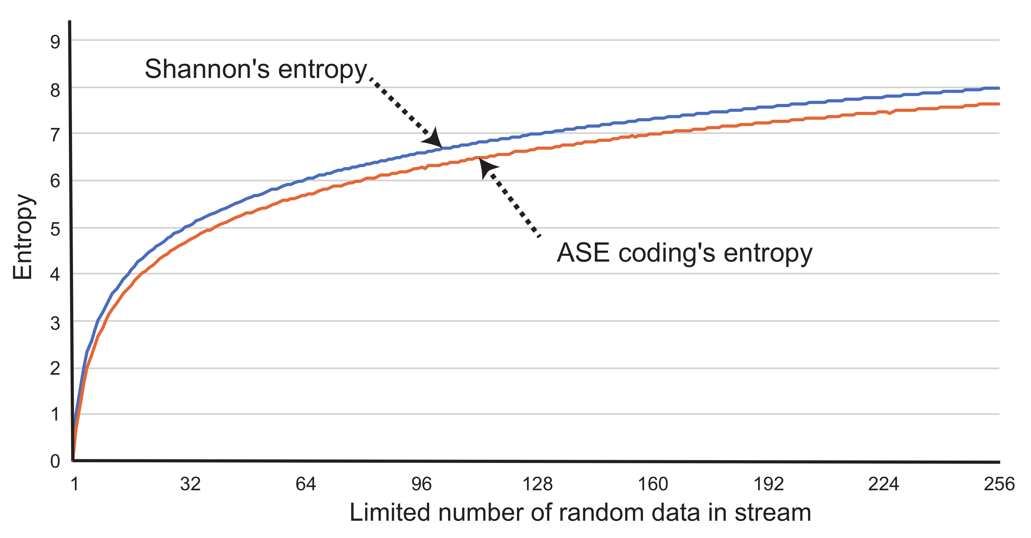
Figure 5 shows comparison between the entropy calculation of the Shannon’s (Equation (
1)) and ASE coding’s (Equation (
2)). This evaluation is performed by calculating the entropies by using an eight-bit width and 10K-byte data stream. The values in the data stream are randomly generated. The horizontal axis of the graph shows the limited number of the random frequency. For example, when the number is 16, the random numbers from 0 to 15 in eight bits are generated and used for the entropy calculation. In the case of ASE coding, we plotted the average by accumulating the entropy calculated at every compression operation. Note that the entropy of the ASE coding does not include Cmark bit. The graph shows that the entropy of ASE coding maintains slightly lower than the Shannon’s. Let us analyze this result below.
Focusing on a part in a data stream from
th to
th data, according to Equation (
1), we can have the equation of the Shannon’s information entropy
, as follows:
Because the part is always negative value regarding any k, the sum of the part is accumulated and linearly decreasing when the interval between and is getting expanded. When we consider where and , the relationship is obvious. Additionally, when is defined as an entropy calculated by a part from to where and , . According to these relationships of the information entropy, we found that ASE coding’s entropy plotted in the graph results lower than the Shannon’s. This means that ASE coding has the possibility to encode data to shorter code than the Shannon’s, because its instantaneous entropy calculation in a small time window works to assign adaptive codes to symbols. This is mainly caused by the entropy culling. It contributes to reduce the number of bits in the codes by purging the occupied entries in the look-up table. However, the Cmark bit must be added to the codes to identify it as whether a compressed code or an original symbol. Thus, the actual data patterns can result a little higher entropy than the Shannon’s.
Let us focus on a theoretical analysis of ASE cording, according to the discussion above. First, we define the compression ratio of the stream-based compression. In a data communication path of a system, the compressor and the decompressor are connected by a physical media. In this setting, we categorize the compression ratio into two types; a micro and a macro compression ratio. The former one is defined at the symbol level. The minimal size of the compressed symbol is only the Cmark bit, which is a single bit. Therefore, the best compression ratio is
, where
s is the number of bits in a symbol. The worst length of the compressed symbol is
bits when it is not hit in the look-up table. The latter case, the macro compression ratio, is defined as a part of data stream between timings
and
when the terminal systems process the part. For example, in a case of a video stream, the decompressor side displays a video frame at a refresh rate. The refresh rate is presented by
for a frame with
L symbols. In this case, the worst bit length of the part is
. Therefore, the best and worst micro compression ratios are defined as
and
, respectively. However, the dynamic performance of the macro compression ratio is not simple, because we need to apply a frequency of data pattern (i.e., data entropy). In the ASE coding case, we have confirmed that the entropy is presented by the number of occupied entries in the look-up table as we discussed above in this section. Thus, we can define the compression ratio of ASE coding, as follows;
where
and
h are the average of the entropy calculation and the hit ratio in the look-up table, respectively, regarding
L symbols between the time interval
and
. Here,
and
h are provided with the effects from a structure/operations of the look-up table and the entropy culling. Let us see the effects against the compression performance in the next experiments below.
4.2. Performance Effect of Near Neighbor Entry Exchange
Here, we evaluate the compression ratio (calculated by the compressed data size/the original data size) with varying distance
d of the nearest neighbor entry exchange.
Figure 6 shows the comparison of the compression ratio by varying
d from 1 to 256. When
, it is equivalent to the LRU (Least Recently Used) method. The smaller
d provides much better complexity for hardware implementation, as we have discussed in the previous section. However, it is expected that the compression ratio should be better when the table operation is near the LRU method. According to the result, the effect of
d is not large against compression ratio. The worst case shows about 8% difference between 1 and 256 of
d. This means that we can use
considering hardware implementation. Thus,
d is not a serious parameter that affects the compression performance. From the next section, we use
and evaluate other sensitive parameters.
4.3. Evaluation for Compression Performance
Next, we evaluate main three parameters that affect to the compression ratio: the number of bits of symbol, the one of the look-up table entries, and the hit counting for the entropy culling.
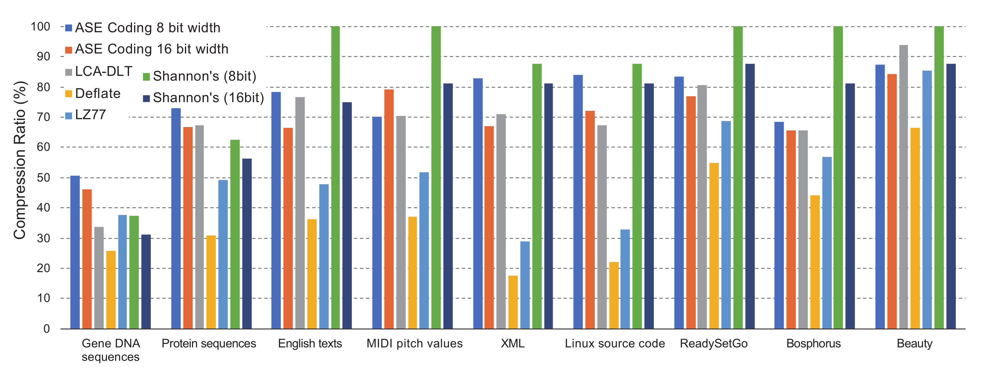
Figure 7 shows the result when the symbol size of ASE coding varies between eight and 16 with comparing to the Shannon’s coding, LCA-DLT and deflate. The symbol size of ASE coding relates to the entropy of the original symbol, because the larger number of symbol bits has higher frequent probability. LCA-DLT and ASE coding work as stream-based and must process statistics by a limited size look-up table. Therefore, it is expected that the Shannon’s and deflate will show a better compression ratio than the ones of LCA-DLT and ASE coding. The graph shows that the compression ratio of ASE coding maintains 50–80%. Performance differences of the text-based cases between ASE coding and deflate are large. However, the ones of 4K images show small performance differences. This means that ASE coding effectively works for high entropy data.
As a reference of buffered and complex compression method, deflate shows a much better compression ratio than ASE coding because it works as universal LZ-based compression with Huffman coding by creating a look-up table that can be dynamically extended.
The Shannon’s coding saturates the assigned code bits until the original symbol width. However, in the case of 16-bit width of Shannon’s, the compression ratios become better than the eight-bit case, because the benchmark data do not have frequency of symbols less than . We can confirm that ASE coding compresses better than the Shannon’s case, as we observed in the previous section.
ASE coding maintains a better compression ratio when the symbol width is 16-bits. However, the benchmark of the MIDI pitch values shows worse. Therefore, we can understand that the symbol width is a sensitive parameter for ASE coding. However, we have a minimal guideline to decide the symbol width. The width should not be misaligned to the data generated from application. We recommend using a symbol width that is one or multiple times of the data width generated from the target application. In this evaluation, we confirmed that the guideline works well.
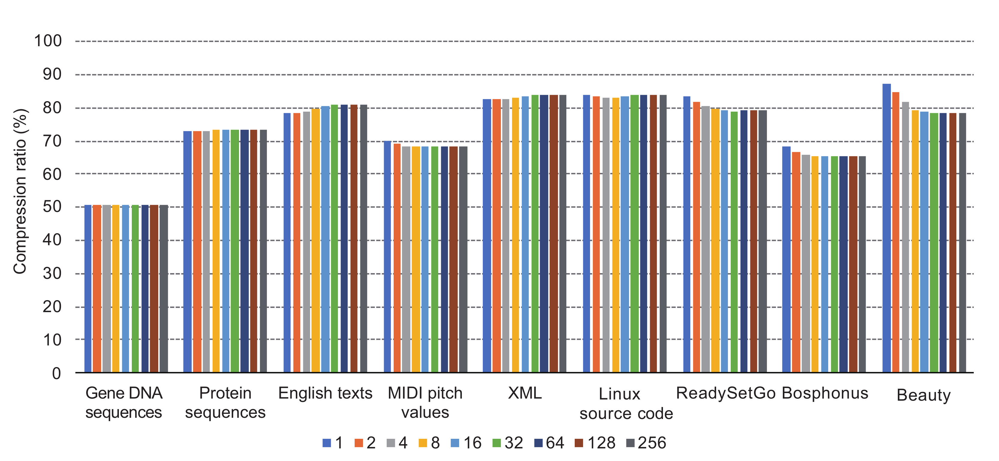
Figure 8 shows the analysis when the number of look-up tables varies from four to 256. The DNA sequence is not affected by the number of entries, because the data consist of combinations of only four ASCII characters. This is caused by a reason why all ASCII characters of the sequence are cached in the table, even if the number of entries in the table is four. However, the entropy culling is working to remove those occupied entries. Although the entropy calculation generates always shorter mask bits, table hit ratio is not affected by the table size. Therefore, the compression ratios among different table sizes do not change in this experiment. On the other hand, the other cases show that all table entries are occupied. When the number of entries is too small,
m from the entropy calculation becomes always
M. This finally degrades compression ratio. Although the compression ratio becomes better as the number of table entries is increased, it degrades again when the number of entries is too large. This means that we need to adjust the number of table entries, depending on entropy of streaming data.
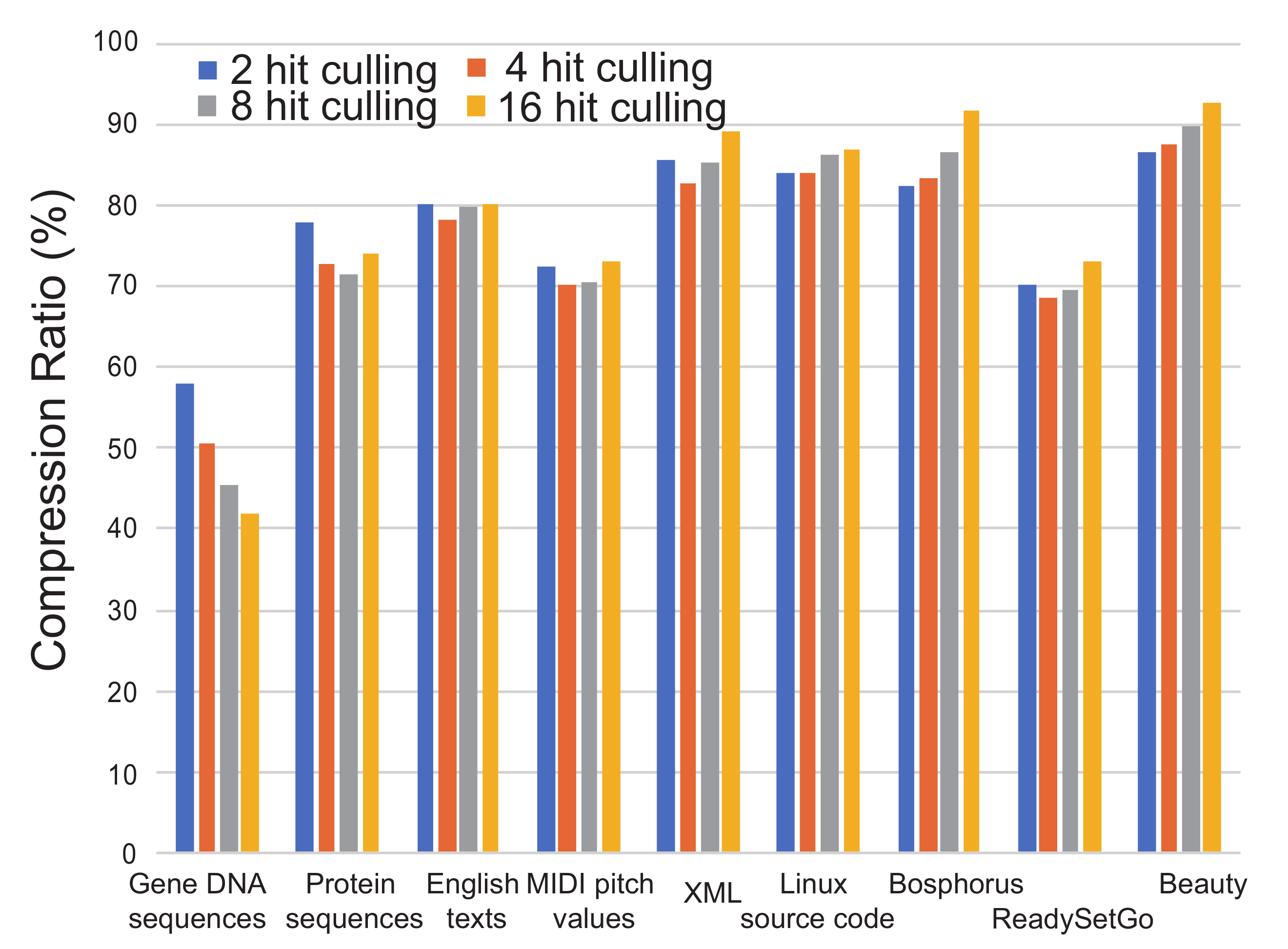
Figure 9 shows the analysis when the setting of the entropy culling is varied from two to 16 hits. When the culling frequency is too high (i.e., the counter is set to a small number), even though the compressed symbol becomes short, entries in the table are often invalidated. Besides when the culling frequency is low, the compressed symbol becomes larger. Thus, these cases cause bad compression ratios. This means that the number of hit counting in the entropy culling is inevitably decided by a heuristic approach. According to the experiment, it can be a good decision to use four as the hit counting. However, it is dependent on the frequency of data patterns that appeared in a data stream.
As we have seen in the evaluations regarding the parameters in ASE coding above, we need to adjust the numbers of the symbol bits, the entries in the look-up table, and the entropy culling’s hit counter, depending on data frequency of target application.
4.4. Evaluation for Hardware Implementation
We have implemented the compression/decompression modules as explained in the previous section. Our implementation is targeted to Xilinx Kintex series FPGA. The compressor module, with 16-bit original symbol for the input, 256 look-up table entries, and eight-bit output of serializer, needs 4500 registers and 4500 LUTs. The number of registers of the compressor can be estimated to about 1.1 times of the number of bits in the look-up table (i.e., ). The number of LUTs is almost the same as the number of registers. The decompressor uses the same number of registers as the compressor’s although the number of LUTs decreases to 0.7 times of the one of compressor. This means that the amount of the combination logic in the decompressor is smaller than the one of compressor. The compressor and the decompressor, respectively, work at 250 MHz. Those process an original symbol by four cycles in each data path of compression/decompression from its input to output where the pipeline stages are organized with the serialize/deserialize operation from/to the original symbols, a look-up table operation, the original/compressed symbol generation, and an output latch. The compressor side can be fully pipelined.
However, a bottleneck stays at the part in the decompressor where m plus Cmark bits are extracted from the compressed data stream D, because the extracted number of bits is not deterministic before the Cmark is evaluated. Additionally, this extraction part must be performed in a single cycle, because the operations of the Cmark evaluation, the entropy calculation, and the m bit extraction from the compressed stream are not dividable. This would become drawback of decompression speed when we try to parallelize the compression/decompression against a single data stream, although the parallelization makes the bandwidth high. For example, when two compression modules are parallelized and pick up original symbols at first and at the second from an input data stream, the compressor side outputs compressed symbols and in this order. This is easily parallelized because the size of original symbols is fixed. However, the size of the compressed symbol is variable. The parallelized decompressors must analyze the sizes of and and its Cmark bits by analyzing in this order. Therefore, if it is widely parallelized to aim higher bandwidth, the decompressor needs to analyze the first Cmark bits and extracts the compressed symbols, and then the next decompressor can analyze the subsequent Cmark bit. This would cause a large latency and become a bottleneck of the communication path. However, in the case of the FPGA, we confirmed that the number of the parallelism can be up to eight at 250MHz. This achieves 2Gbyte/sec. This is equivalent to four lane PCI Gen2 that is currently one of the typical fast I/O standards.
On the other hand, if the faster I/O is required, multiple compressors/decompressors can receive multiple data streams in fully parallel. For example, if a data stream can be divided to eight streams, and then those are sent respectively to the compressors in parallel. The decompressors also receive those streams in parallel. In this case, we do not need to care the bottleneck regarding the number of bits of a compressed data. Because ASE coding module can be implemented in a very small resources, the FPGA can include hundreds of modules. Therefore, applying ASE coding, we can implement 10Tbyte/sec order compression/decompression in the FPGA.
Here, let us compare the resources needed by LCA-DLT that performs the compression ratios shown in
Figure 7. The compressor consists of about 9K registers and 8K LUTs, which works at 200 MHz. ASE coding is implemented by approximately half the resources of LCA-DLT and also works at 25% higher clock frequency.
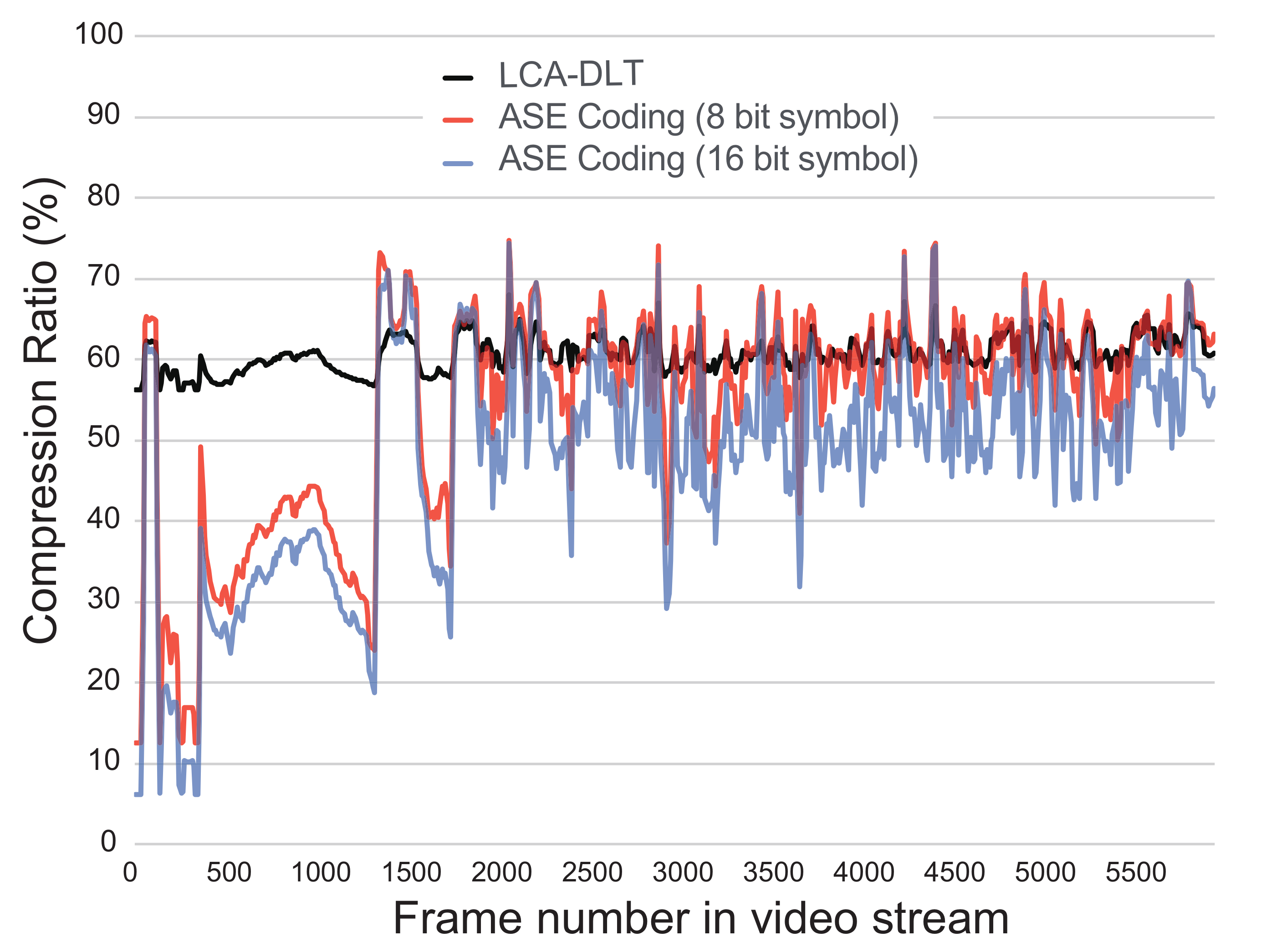
Using ASE coding, we have developed a realtime compression system of HDMI data stream. The speed of the compression is 150MHz with 24-bit wide color pixel stream that consists of YUV444 color data.
Figure 10 shows the realtime compression ratio of every frame during eight minutes of a full HD computer graphics movie that presents battles of space fighters. During the experiment, we used two compressors of ASE coding with eight- and 16-bit input symbol. We compare those with an LCA-DLT with a compressor of eight-bit symbol (16-bit input) and 256 look-up table entries. Both ratios of ASE coding become low in the beginning of video, because the first 1500 frames are almost black frame. This means that short codes are generated adaptively due to the entropy culling. Here, the ASE coding of 16-bit symbol input results better compression ratio than the one of eight-bit because the entropy culling works better in the case of 16 bits than the one of eight bits. Totally, both results of ASE coding show better compression ratios than LCA-DLT. Thus, the compressed data associated from the entropy calculation work adaptively to decide the shortest bits for the instant data frequency.


