A Novel Method for Inference of Chemical Compounds of Cycle Index Two with Desired Properties Based on Artificial Neural Networks and Integer Programming

Abstract

Inference of chemical compounds with desired properties is important for drug design, chemo-informatics, and bioinformatics, to which various algorithmic and machine learning techniques have been applied. Recently, a novel method has been proposed for this inference problem using both artificial neural networks (ANN) and mixed integer linear programming (MILP). This method consists of the training phase and the inverse prediction phase. In the training phase, an ANN is trained so that the output of the ANN takes a value nearly equal to a given chemical property for each sample. In the inverse prediction phase, a chemical structure is inferred using MILP and enumeration so that the structure can have a desired output value for the trained ANN. However, the framework has been applied only to the case of acyclic and monocyclic chemical compounds so far. In this paper, we significantly extend the framework and present a new method for the inference problem for rank-2 chemical compounds (chemical graphs with cycle index 2). The results of computational experiments using such chemical properties as octanol/water partition coefficient, melting point, and boiling point suggest that the proposed method is much more useful than the previous method.

1. Introduction

Inference of chemical compounds with desired properties is important for computer-aided drug design. Since drug design is one of the major targets of chemo-informatics and bioinformatics, it is also important in these areas. Indeed, this problem has been extensively studied in chemo-informatics under the name of inverse QSAR/QSPR [1,2], where QSAR/QSPR denotes Quantitative Structure Activity/Property Relationships. Since chemical compounds are usually represented as undirected graphs, this problem is important also from graph theoretic and algorithmic viewpoints.

Inverse QSAR/QSPR is often formulated as an optimization problem to find a chemical graph maximizing (or minimizing) an objective function under various constraints, where objective functions reflect certain chemical activities or properties. In many cases, objective functions are derived from a set of training data consisting of known molecules and their activities/properties using statistical and machine learning methods.

In both forward and inverse QSAR/QSPR, chemical graphs are often represented as vectors of real or integer numbers because it is difficult to directly handle graphs using statistical and machine learning methods. Elements of these vectors are called descriptors in QSAR/QSPR studies, and these vectors correspond to feature vectors in machine learning. Using these chemical descriptors, various heuristic and statistical methods have been developed for finding optimal or nearly optimal graph structures under given objective functions [1,3,4]. In many cases, inference or enumeration of graph structures from a given feature vector is a crucial subtask in these methods. Various methods have been developed for this enumeration problem [5,6,7,8] and the computational complexity of the inference problem has been analyzed [9,10,11]. On the other hand, enumeration in itself is a challenging task, since the number of molecules (i.e., chemical graphs) with up to 30 atoms (vertices) C, N, O, and S, may exceed ${10}^{60}$ [12].

As in many other fields, Artificial Neural Network (ANN) and deep learning technologies have recently been applied to inverse QSAR/QSPR. For example, variational autoencoders [13], recurrent neural networks [14,15], and grammar variational autoencoders [16] have been applied. In these approaches, new chemical graphs are generated by solving a kind of inverse problems on neural networks, where neural networks are trained using known chemical compound/activity pairs. However, the optimality of the solution is not necessarily guaranteed in these approaches. In order to guarantee the optimality, a novel approach has been proposed [17] for ANNs with ReLU activation functions and sigmoid activation functions, using mixed integer linear programming (MILP). In their approach, activation functions on neurons are efficiently encoded as piece-wise linear functions so as to represent ReLU functions exactly and sigmoid functions approximately.

Recently, a new framework has been proposed [18,19,20] by combining two previous approaches; efficient enumeration of tree-like graphs [5], and MILP-based formulation of the inverse problem on ANNs [17]. This combined framework for inverse QSAR/QSPR mainly consists of two phases, one for constructing a prediction function to a chemical property, and the other for constructing graphs based on the inverse of the prediction function. The first phase solves (I) Prediction Problem, where a prediction function ${\psi }_{\mathcal{N}}$ on a chemical property $\pi$ is constructed with an ANN $\mathcal{N}$ using a data set of chemical compounds G and their values $a\left(G\right)$ of $\pi$. The second phase solves (II) Inverse Problem, where (II-a) given a target value $y^{*}$ of the chemical property $\pi$, a feature vector $x^{*}$ is inferred from the trained ANN $\mathcal{N}$ so that ${\psi }_{\mathcal{N}}\left(x^{*}\right)$ is close to $y^{*}$ and (II-b) then a set of chemical structures $G^{*}$ such that $f\left(G^{*}\right)=x^{*}$ is enumerated. In (II-b) of the above-mentioned previous methods [18,19,20], an MILP is formulated for acyclic chemical compounds. Their methods were applicable only to acyclic chemical graphs (i.e., tree-structured chemical graphs), where the ratio of acyclic chemical graphs in a major chemical database (PubChem) is 2.91%. Afterward, Ito et al. [21] designed a method of inferring monocyclic chemical graphs (chemical graphs with cycle index or rank 1) by formulating a new MILP and using an efficient algorithm for enumerating monocyclic chemical graphs [22]. This still leaves a big limitation because the ratio of acyclic and monocyclic chemical graphs in the chemical database PubChem is only 16.26%.

To break this limitation, we significantly extend the MILP-based approach for inverse QSAR/QSPR so that “rank-2 chemical compounds” (chemical graphs with cycle index or rank 2) can be efficiently handled, where the ratio of chemical graphs with rank at most 2 in the database PubChem is 44.5%. Note that there are three different topological structures, called polymer-topologies over all rank-2 chemical compounds. In particular, we propose a novel MILP formulation for (II-a) along with a new set of descriptors. One big advantage of this new formulation is that an MILP instance has a solution if and only if there exists a rank-2 chemical graph satisfying given constraints, which is useful to significantly reduce redundant search in (II-b). We conducted computational experiments to infer rank-2 chemical compounds on several chemical properties.

The paper is organized as follows. Section 2.1 introduces some notions on graphs, a modeling of chemical compounds, and a choice of descriptors. Section 2.2 reviews the framework for inferring chemical compounds based on ANNs and MILPs. Section 2.3 introduces a method of modeling rank-2 chemical graphs with different cyclic structures in a unified way and proposes an MILP formulation that represents a rank-2 chemical graph G of n vertices, where our MILP requires only $O\left(n\right)$ variables and constraints when the maximum height of subtrees in G is constant. Section 3 reports the results on some computational experiments conducted for chemical properties such as octanol/water partition coefficient, melting point, and boiling point. Section 4 makes some concluding remarks. Appendix A provides the detail of all variables and constraints in our MILP formulation.

2. Materials and Methods

2.1. Preliminary

This section introduces some notions and terminology on graphs, a modeling of chemical compounds, and our choice of descriptors.

2.1.1. Multigraphs and Graphs

Let $\mathbb{R}$ and $\mathbb{Z}$ denote the sets of reals and non-negative integers, respectively. For two integers a and b, let $[a,b]$ denote the set of integers i with $a\le i\le b$.

Multigraphs

A multigraph is defined to be a pair $(V,E)$ of a vertex set V and an edge set E such that each edge $e\in E$ joins two vertices $u,v\in V$ (possibly $u=v$) and the vertices u and v are called the end-vertices of the edge e, and let $V\left(e\right)$ denote the set of the end-vertices of an edge $e\in E$, where an edge e with $\left|V\right(e\left)\right|=1$ is called a loop. We denote the vertex and edge sets of a multigraph M by $V\left(M\right)$ and $E\left(M\right)$, respectively. A path with end-vertices u and v is called a $u,v$-path, and the length of a path is defined to be the number of edges in the path.

Let M be a multigraph. An edge $e\in E\left(M\right)$ is called multiple (to an edge $e^{\prime }\in E\left(M\right)$) if there is another edge $e^{\prime }\in E\left(M\right)$ with $V\left(e\right)=V\left(e^{\prime }\right)$. For a vertex $v\in V\left(M\right)$, the set of neighbors of v in M is denoted by $N_M\left(v\right)$, and the degree ${\mathrm{deg}}_M\left(v\right)$ of v is defined to be the number of times an edge in $E\left(M\right)$ is incident to v; i.e., ${\mathrm{deg}}_M\left(v\right)=\left|\right\{e\in E\left(M\right)\mid v\in V\left(e\right),\left|V\left(e\right)\right|=2\left\}\right|+2\left|\right\{e\in E\left(M\right)\mid v\in V\left(e\right),\left|V\left(e\right)\right|=1\left\}\right|$. A multigraph is called simple if it has no loop and there is at most one edge between any two vertices. We observe that the sum of the degrees over all vertices is twice the number of edges in any multigraph M; i.e.,

$$2\left|E\left(M\right)\right|=\sum _{v\in V\left(M\right)}{\mathrm{deg}}_M\left(v\right).$$

For a subset X of vertices in M, let $M-X$ denote the multigraph obtained from M by removing the vertices in X and any edge incident to a vertex in X. An operation of subdividing a non-loop edge (resp., loop) $e\in E\left(M\right)$ with $V\left(e\right)=\{v_1,v_2\}$ (resp., $V\left(e\right)=\{v_1=v_2\}$) is to replace e with two new edges $e_1$ and $e_2$ incident to a new vertex $v_e$ such that each $e_i$ is incident to $v_i$. An operation of contracting a vertex u of degree 2 in M is to replace the two edges $uv$ and $u{v}^{\prime }$ incident to u with a single edge $v{v}^{\prime }$ removing vertex u, where the resulting edge is a loop when $v=v^{\prime }$. The rank $\mathrm{r}\left(M\right)$ of a multigraph M is defined to be the minimum number of edges to be removed to make the multigraph acyclic. We call a multigraph M with $\mathrm{r}\left(M\right)=k$ a rank-k graph. Let $V_{\mathrm{deg},i}\left(M\right)$ denote the set of vertices of degree i in M. The core $\mathrm{Cr}\left(M\right)$ of M is defined to be an induced subgraph $M^{*}$ that is obtained from $M^{\prime }:=M$ by setting $M^{\prime }:=M^{\prime }-V_{\mathrm{deg}},1\left(M^{\prime }\right)$ repeatedly until $M^{*}$ contains at most two vertices or consists of vertices of degree at least 2. The core $M^{*}$ of a connected multigraph M consists of a single vertex (resp., two vertices) if and only if M is a tree with an even (resp., odd) diameter. A vertex (resp., an edge) in M is called a core vertex (resp., core edge) if it is contained in the core of M and is called a non-core vertex (resp., non-core edge) otherwise. The core size $\mathrm{cs}\left(M\right)$ is defined to be the number of core vertices of M, and the core height $\mathrm{ch}\left(M\right)$ is defined to be the maximum length of a path between a vertex $v\in V\left(M^{*}\right)$ to a leaf of M without passing through any core edge. The set of non-core edges induces a collection of subtrees, each of which we call a non-core component of M, where each non-core component C contains exactly one core vertex $v_C$ and we regard C as a tree rooted at $v_C$. Let C be a non-core component of M. The height $\mathrm{height}\left(v\right)$ of a vertex v in C is defined to be the maximum length of a path from v to a leaf u in the descendants of v.

A multigraph is called a polymer topology if it is connected and the degree of every vertex is at least 3. Tezuka and Oike [23] pointed out that a classification of polymer topologies will lay a foundation for elucidation of structural relationships between different macro-chemical molecules and their synthetic pathways. For integers $r\ge 0$ and $d\ge 3$, let $\mathcal{PT}(r,d)$ denote the set of all rank-r polymer topologies with maximum degree at most d. Figure 1 illustrates the three rank-2 polymer topologies in $\mathcal{PT}(2,4)$.

Figure 1. An illustration of the three rank-2 polymer topologies $M_1,M_2,M_3\in \mathcal{PT}(2,4)$.

For a polymer topology M, the least simple graph $S\left(M\right)$ of M is defined to be a simple graph obtained from M by subdividing each loop in M with two new vertices of degree 2 and subdividing all multiple edges (except for one) between every two adjacent vertices in M. Note that $\left|V\right(S\left(M\right)\left)\right|=\left|V\right(M\left)\right|+r+s$ for the rank r of M and the number s of loops in M.

The polymer topology $\mathrm{Pt}\left(M\right)$ of a multigraph M with $\mathrm{r}\left(M\right)\ge 2$ is defined to be a multigraph $M^{\prime }$ of degree at least 3 that is obtained from the core $\mathrm{Cr}\left(M\right)$ by contracting all vertices of degree 2. Note that $\mathrm{r}\left(\mathrm{Pt}\right(M\left)\right)=\mathrm{r}\left(M\right)$. Figure 2a–c illustrate the least simple graph $S\left(M\right)$ of each polymer topology $M\in \mathcal{PT}(2,4)$, where Figure 2d illustrates a graph that contains all least simple graphs.

Figure 2. An illustration of the least simple graphs of the rank-2 polymer topologies $M_1,M_2,M_3\in \mathcal{PT}(2,4)$ in Figure 1 and a scheme graph $(K,\mathcal{E})$: (a) $S\left(M_1\right)$; (b) $S\left(M_2\right)$; (c) $S\left(M_3\right)$; (d) a scheme graph $(K=(\{u_1,u_2,u_3,u_4\},E),\mathcal{E}=(E_1,E_2,E_3))$ where each edge $u_i{u}_j$ is directed from one end-vertex $u_i$ to the other end-vertex $u_j$ with $i<j$, and $E_1=\{a_1=(u_1,u_4),a_2=(u_2,u_3),a_3=(u_2,u_4)\}$, $E_2=\{a_4=(u_1,u_2),a_5=(u_3,u_4)\}$ and $E_3=\{a_6=(u_1,u_2),a_7=(u_3,u_4)\}$, and the edges in $E_1$ (resp., $E_2$ and $E_3$) are depicted with dashed (resp., dotted and solid) lines.

Graphs

Let $H=(V,E)$ be a graph with a set V of vertices and a set E of edges. Define the 1-path connectivity ${\kappa }_1\left(H\right)$ of H to be ${\sum }_{uv\in E}1/\sqrt{{\mathrm{deg}}_H\left(u\right){\mathrm{deg}}_H\left(v\right)}$.

Let H be a rank-2 connected graph such that the maximum degree is at most 4. We see that H contains two vertices $v_a$ and $v_b$ such that either there are three disjoint paths between $v_a$ and $v_b$ or H contains two edge disjoint cycles C and $C^{\prime }$, which are joined with a path between $v_a$ and $v_b$ (possibly $v_a=v_b$). We introduce the topological parameter $\theta \left(H\right)$ of rank-2 connected graph H as follows. When H has three disjoint paths between $v_a$ and $v_b$, define $\theta \left(H\right)$ to be the minimum number of edges along a path between $v_a$ and $v_b$. When H contains two edge disjoint cycles C and $C^{\prime }$, which are joined with a path P between $v_a$ and $v_b$ (possibly $v_a=v_b$), define $\theta \left(H\right)$ to be $-\left|E\right(P\left)\right|$.

For positive integers $a,b$ and c with $b\ge 2$, let $T(a,b,c)$ denote the rooted tree such that the number of children of the root is a, the number of children of each non-root internal vertex is b and the distance from the root to each leaf is c. In the rooted tree $T(a,b,c)$, we denote the vertices by $v_1,v_2,\dots ,v_n$ ($n=a(b^c-1)/(b-1)+1$) with a breadth-first-search order, and denote the edge between a vertex $v_i$ with $i\in [2,n]$ and its parent by $e_i$. For each vertex $v_i$ in $T(a,b,c)$, let $\mathrm{Cld}\left(i\right)$ denote the set of indices j such that $v_j$ is a child of $v_i$, and $\mathrm{prt}\left(i\right)$ denote the index j such that $v_j$ is the parent of $v_i$ when $i\in [2,n]$.

2.1.2. Modeling of Chemical Compounds

Chemical Graphs

We represent the graph structure of a chemical compound as a graph with labels on vertices and multiplicity on edges in a hydrogen-suppressed model. Nearly 68.5% (resp., 99%) of the rank-2 chemical graphs with at most 200 non-hydrogen atoms registered in chemical database PubChem have a maximum degree at most 3 (resp., 4) for all non-core vertices in the hydrogen-suppressed model.

Let $\Lambda$ be a set of labels, each of which represents a chemical element such as C (carbon), O (oxygen), N (nitrogen) and so on, where we assume that $\Lambda$ does not contain H (hydrogen). Let $\mathrm{mass}\left(\mathtt{a}\right)$ and $\mathrm{val}\left(\mathtt{a}\right)$ denote the mass and valence of a chemical element $\mathtt{a}\in \Lambda$, respectively. In our model, we use integers ${\mathrm{mass}}^{*}\left(\mathtt{a}\right)=\lfloor 10·\mathrm{mass}\left(\mathtt{a}\right)\rfloor$, $\mathtt{a}\in \Lambda$ and assume that each chemical element $\mathtt{a}\in \Lambda$ has a unique valence $\mathrm{val}\left(\mathtt{a}\right)\in [1,4]$.

We introduce a total order < over the elements in $\Lambda$ according to their mass values; i.e., we write $\mathtt{a}<\mathtt{b}$ for chemical elements $\mathtt{a},\mathtt{b}\in \Lambda$ with $\mathrm{mass}\left(\mathtt{a}\right)<\mathrm{mass}\left(\mathtt{b}\right)$. Choose a set ${\Gamma }_{<}$ of tuples $\gamma =(\mathtt{a},\mathtt{b},k)\in \Lambda \times \Lambda \times [1,3]$ such that $\mathtt{a}<\mathtt{b}$. For a tuple $\gamma =(\mathtt{a},\mathtt{b},k)\in \Lambda \times \Lambda \times [1,3]$, let $\overline{\gamma }$ denote the tuple $(\mathtt{b},\mathtt{a},k)$. Set ${\Gamma }_{>}=\{\overline{\gamma }\mid \gamma \in {\Gamma }_{<}\}$, ${\Gamma }_{=}=\{(\mathtt{a},\mathtt{a},k)\mid \mathtt{a}\in \Lambda ,k\in [1,3]\}$ and $\Gamma ={\Gamma }_{<}\cup {\Gamma }_{=}$. a pair of two atoms $\mathtt{a}$ and $\mathtt{b}$ joined with a bond of multiplicity k is denoted by a tuple $\gamma =(\mathtt{a},\mathtt{b},k)\in \Gamma$, called  the adjacency-configuration of the atom pair.

We use a hydrogen-suppressed model because hydrogen atoms can be added at the final stage. a chemical graph over $\Lambda$ and $\Gamma$ is defined to be a tuple $G=(H,\alpha ,\beta )$ of a graph $H=(V,E)$, a function $\alpha :V\to \Lambda$ and a function $\beta :E\to [1,3]$ such that

(i)

H is connected;

(ii)

${\sum }_{uv\in E}\beta \left(uv\right)\le \mathrm{val}\left(\alpha \left(u\right)\right)$ for each vertex $u\in V$; and

(iii)

$\left(\alpha \right(u),\alpha (v),\beta (uv\left)\right)\in \Gamma$ for each edge $uv\in E$.

Let $\mathcal{G}(\Lambda ,\Gamma )$ denote the set of chemical graphs over $\Lambda$ and $\Gamma$.

Descriptors

In our method, we use only graph-theoretical descriptors for defining a feature vector, which facilitates our designing an algorithm for constructing graphs. Given a chemical graph $G=(H,\alpha ,\beta )$, we define a feature vector $f\left(G\right)$ that consists of the following 14 kinds of descriptors:

-

$n\left(G\right)$: the number of vertices in G;

-

$\mathrm{cs}\left(G\right)$: the core size of G;

-

$\mathrm{ch}\left(G\right)$: the core height of G;

-

${\kappa }_1\left(G\right)$: the 1-path connectivity of G;

-

${\mathrm{dg}}_i\left(G\right)$ ($i\in [1,4]$): the number of vertices of degree i in G;

-

${\mathrm{ce}}_{\mathtt{a}}^{\mathrm{co}}\left(G\right)$ ($\mathtt{a}\in \Lambda )$: the number of core vertices with chemical element $\mathtt{a}\in \Lambda$;

-

${\mathrm{ce}}_{\mathtt{a}}^{\mathrm{nc}}\left(G\right)$ ($\mathtt{a}\in \Lambda )$: the number of non-core vertices with chemical element $\mathtt{a}\in \Lambda$;

-

$\overline{\mathrm{ms}}\left(G\right)$: the average of ${\mathrm{mass}}^{*}$ of atoms in G;

-

$b_k^{\mathrm{co}}\left(G\right)$ ($k\in [2,3]$): the number of double and triple bonds in core edges;

-

$b_k^{\mathrm{nc}}\left(G\right)$ ($k\in [2,3]$): the number of double and triple bonds in non-core edges;

-

${\mathrm{ac}}_{\gamma }^{\mathrm{co}}\left(G\right)$ ($\gamma =(\mathtt{a},\mathtt{b},k)\in \Gamma$): the number of adjacency-configurations $(\mathtt{a},\mathtt{b},k)$ of core edges;

-

${\mathrm{ac}}_{\gamma }^{\mathrm{nc}}\left(G\right)$ ($\gamma =(\mathtt{a},\mathtt{b},k)\in \Gamma$): the number of adjacency-configurations $(\mathtt{a},\mathtt{b},k)$ of non-core edges;

-

$\theta \left(H\right)$: the topological parameter of H; and

-

$n_{\mathtt{H}}\left(G\right)$: the number of hydrogen atoms to be included in G; i.e.,

$n_{\mathtt{H}}\left(G\right)={\sum }_{\mathtt{a}\in \Lambda }\mathrm{val}\left(\mathtt{a}\right)({\mathrm{ce}}_{\mathtt{a}}^{\mathrm{co}}\left(G\right)+{\mathrm{ce}}_{\mathtt{a}}^{\mathrm{nc}}\left(G\right))-2(n\left(G\right)+1+b_2^{\mathrm{co}}\left(G\right)+b_2^{\mathrm{nc}}\left(G\right)+2b_3^{\mathrm{co}}\left(G\right)+2b_3^{\mathrm{nc}}\left(G\right))$.

The number k of descriptors in our feature vector $x=f\left(G\right)$ is $k=2|\Lambda |+2|\Gamma |+15$.

2.2. A Method for Inferring Chemical Graphs

This section reviews the framework that solves the inverse QSAR/QSPR by using MILPs [18]. For a specified chemical property $\pi$ such as boiling point, we denote by $a\left(G\right)$ the observed value of the property $\pi$ for a chemical compound G. As the Phase 1, we solve (I) Prediction Problem with the following three steps.

Phase 1.

Step 1: Let $\mathrm{DB}$ be a set of chemical graphs. For a specified chemical property $\pi$, choose a class $\mathcal{G}$ of graphs such as acyclic graphs or monocyclic graphs. Prepare a data set $D_{\pi }=\{G_i\mid i=1,2,\dots ,m\}\subseteq \mathcal{G}\cap \mathrm{DB}$ such that the value $a\left(G_i\right)$ of each chemical graph $G_i$, $i=1,2,\dots ,m$ is available. Set reals $\underline{a},\overline{a}\in \mathbb{R}$ so that $\underline{a}\le a\left(G_i\right)\le \overline{a}$, $i=1,2,\dots ,m$. See Figure 3 for an illustration of Step 1.

Figure 3. An illustration of Step 1: A data set $D_{\pi }$ of chemical graphs $G_i$, $i=1,2,\dots ,m$ in a class $\mathcal{G}$ of graphs whose values $a\left(G_i\right)\in [\underline{a},\overline{a}]$ of a chemical property $\pi$ are available.

Step 2: Introduce a feature function $f:\mathcal{G}\to {\mathbb{R}}^k$ for a positive integer k. We call $f\left(G\right)$ the feature vector of $G\in \mathcal{G}$, and call each entry of a vector $f\left(G\right)$ a descriptor of G. See Figure 4 for an illustration of Step 2.

Figure 4. An illustration of Step 2: Each chemical graph $G\in \mathcal{G}$ is mapped to a vector $f\left(G\right)$ in a feature vector space ${\mathbb{R}}^k$ for some positive integer k.

Step 3: Construct a prediction function ${\psi }_{\mathcal{N}}$ with an ANN $\mathcal{N}$ that, given a vector in ${\mathbb{R}}^k$, returns a real in the range $[\underline{a},\overline{a}]$ so that ${\psi }_{\mathcal{N}}\left(f\left(G\right)\right)$ takes a value nearly equal to $a\left(G\right)$ for many chemical graphs in D. See Figure 5 for an illustration of Step 3.

Figure 5. An illustration of Step 3: A prediction function ${\psi }_{\mathcal{N}}$ from the feature vector space ${\mathbb{R}}^k$ to the range $[\underline{a},\overline{a}]$ is constructed based on an ANN $\mathcal{N}$.

Next we explain how to solve the inverse problem to the prediction in Phase 1 using an MILP formulation. A vector $x\in {\mathbb{R}}^k$ is called admissible if there is a graph $G\in \mathcal{G}$ such that $f\left(G\right)=x$ [18]. Let $\mathcal{A}$ denote the set of admissible vectors $x\in {\mathbb{R}}^k$. In this paper, we use the range-based method to define an applicability domain (AD) [24] to our inverse QSAR/QSPR. Set $\underline{x_j}$ and $\overline{x_j}$ to be the minimum and maximum values of the j-th descriptor $x_j$ in $f\left(G_i\right)$ over all graphs $G_i$, $i=1,2,\dots ,m$ (where we possibly normalize some descriptors such as ${\mathrm{ce}}_{\mathtt{a}}^{\mathrm{co}}\left(G\right)$, which is normalized with ${\mathrm{ce}}_{\mathtt{a}}^{\mathrm{co}}\left(G\right)/n\left(H\right)$). Define our AD $\mathcal{D}$ to be the set of vectors $x\in {\mathbb{R}}^k$ such that $\underline{x_j}\le x_j\le \overline{x_j}$ for the variable $x_j$ of each j-th descriptor, $j=1,2,\dots ,k$. As the second phase, we solve (II) Inverse Problem for the inverse QSAR/QSPR by treating the following inference problems.

(II-a) Inference of Vectors

Input: A real $y^{*}\in [\underline{a},\overline{a}]$.

Output: Vectors $x^{*}\in \mathcal{A}\cap \mathcal{D}$ and $g^{*}\in {\mathbb{R}}^h$ such that ${\psi }_{\mathcal{N}}\left(x^{*}\right)=y^{*}$ and $g^{*}$ forms a chemical graph $G^{*}\in \mathcal{G}$ with $f\left(G^{*}\right)=x^{*}$.

(II-b) Inference of Graphs

Input: A vector $x^{*}\in \mathcal{A}\cap \mathcal{D}$.

Output: All graphs $G^{*}\in \mathcal{G}$ such that $f\left(G^{*}\right)=x^{*}$.

To treat Problem (II-a), we use MILPs for inferring vectors in ANNs [17]. In MILPs, we can easily impose additional linear constraints or fix some variables to specified constants. We include into the MILP a linear constraint such that $x\in \mathcal{D}$ to obtain the next result.

Theorem 1.

Let $\mathcal{N}$ be an ANN with a piecewise-linear activation function for an input vector $x\in {\mathbb{R}}^k$, $n_A$ denote the number of nodes in the architecture and $n_B$ denote the total number of break-points over all activation functions. Then there is an MILP $\mathcal{M}(x,y;{\mathcal{C}}_1)$ that consists of variable vectors $x\in \mathcal{D}(\subseteq {\mathbb{R}}^k)$, $y\in \mathbb{R}$, and an auxiliary variable vector $z\in {\mathbb{R}}^p$ for some integer $p=O(n_A+n_B)$ and a set ${\mathcal{C}}_1$ of $O(n_A+n_B)$ constraints on these variables such that: ${\psi }_{\mathcal{N}}\left(x^{*}\right)=y^{*}$ if and only if there is a vector $(x^{*},y^{*})$ feasible to $\mathcal{M}(x,y;{\mathcal{C}}_1)$.

See Appendix A for the set of constraints to define our AD $\mathcal{D}$ in the MILP $\mathcal{M}(x,y;{\mathcal{C}}_1)$ in Theorem 1.

To attain the admissibility of inferred vector $x^{*}$, we also introduce a variable vector $g\in {\mathbb{R}}^q$ for some integer q and a set ${\mathcal{C}}_2$ of constraints on x and g such that $x^{*}\in \mathcal{A}$ holds in the following sense: $(x^{*},g^{*})$ is feasible to the MILP $\mathcal{M}(x,g;{\mathcal{C}}_2)$ if and only if $g^{*}$ forms a chemical graph $G^{*}\in \mathcal{G}$ with $f\left(G^{*}\right)=x^{*}$. The Phase 2 consists of the next two steps.

Phase 2.

Step 4: Formulate Problem (II-a) as the above MILP $\mathcal{M}(x,y,g;{\mathcal{C}}_1,{\mathcal{C}}_2)$ based on $\mathcal{G}$ and $\mathcal{N}$. Find a set $F^{*}$ of vectors $x^{*}\in \mathcal{A}\cap \mathcal{D}$ such that $(1-\epsilon )y^{*}\le {\psi }_{\mathcal{N}}\left(x^{*}\right)\le (1+\epsilon )y^{*}$ for a tolerance $\epsilon$ set to be a small positive real. See Figure 6 for an illustration of Step 4.

Figure 6. An illustration of Step 4: Given a target value $y^{*}\in [\underline{a},\overline{a}]$, solving MILP $\mathcal{M}(x,y,g;{\mathcal{C}}_1,{\mathcal{C}}_2)$ either delivers a set $F^{*}$ of vectors $x^{*}\in \mathcal{A}\cap \mathcal{D}$ such that $(1-\epsilon )y^{*}\le {\psi }_{\mathcal{N}}\left(x^{*}\right)\le (1+\epsilon )y^{*}$ or detects that no such vector $x$ exists.

Step 5: To solve Problem (II-b), enumerate all graphs $G^{*}\in \mathcal{G}$ such that $f\left(G^{*}\right)=x^{*}$ for each vector $x^{*}\in F^{*}$. See Figure 7 for an illustration of Step 5.

Figure 7. An illustration of Step 5: For each vector $x^{*}\in F^{*}$, all chemical graphs $G^{*}\in \mathcal{G}$ such that $f\left(G^{*}\right)=x^{*}$ are generated.

In this paper, we set a graph class $\mathcal{G}$ to be the set of rank-2 graphs. In Step 4, we solve an MILP $\mathcal{M}(x,g;{\mathcal{C}}_2)$ that is formulated on a novel idea of representing rank-2 chemical graphs, as will be discussed in Section 2.3.2. In Step 5, we use branch-and-bound algorithms for enumerating rank-2 chemical compounds [25,26].

2.3. Representing Rank-2 Chemical Graphs

This section introduces a method of modeling rank-2 chemical graphs with different cyclic structures in a unified way and proposes an MILP formulation that represents a rank-2 chemical graph G of n vertices.

2.3.1. Scheme Graphs and Tree-Extensions

Given positive integers $n^{*}$ and p, a graph with $n^{*}$ vertices and p edges can be represented as a subgraph of a complete graph $K_{n^{*}}$ with $n^{*}(n^{*}-1)/2$ edges. However, formulating this as an MILP may require to prepare $\Omega \left({\left(n^{*}\right)}^2\right)$ variables and constraints. To reduce the number of variables and constraints in an MILP that represents a rank-2 graph, we decompose a rank-2 graph G into the core and non-core of G so that the core is represented by one of the three rank-2 polymer topologies and the non-core is a collection of trees in which the height is bounded by the core height of G. We do not specify how many subtrees will be attached to each edge in the polymer topology in advance, since otherwise we would need a different MILP for a distinct combination of such assignments of subtrees. Instead we allow each edge in a polymer topology to collect a necessary number of subtrees in our MILP (see the next section for more detail). In this section, we introduce a “scheme graph” to represent three possible rank-2 polymer topologies, an “extension” of the scheme graph to represent the core of a rank-2 graph and a “tree-extension” to represent a combination of the core and non-core of a rank-2 graph, so that any of the three kinds of rank-2 polymer topologies can be selected in a single MILp formulation.

Scheme Graphs

Formally, we define the scheme graph for rank 2 to be a pair $(K,\mathcal{E})$ of a multigraph K and an ordered partition $\mathcal{E}=(E_1,E_2,E_3)$ of the edge set $E\left(K\right)$. Figure 2d illustrates the scheme graph $(K=(\{u_1,u_2,u_3,u_4\},E),\mathcal{E}=(E_1,E_2,E_3))$. An edge in $E_1$ is called a semi-edge, an edge in $E_2$ is called a virtual edge and an edge in $E_3$ is called a real edge.

Extensions of Scheme Graphs

Based on the scheme graph $(K,\mathcal{E})$, we construct the core of a rank-2 graph H as an “extension,” which is defined as follows (see also Figure 8). The extension $H_{\mathrm{core}}$ in Figure 9a An extension of the scheme graph $(K,\mathcal{E})$ is defined to be a simple graph obtained from K by using each real edge $e=uv\in E_3$, by eliminating or replacing each virtual edge $e=uv\in E_2$ (resp., semi-edge $e=uv\in E_1$) with a $u,v$-path of length at least two (resp., 1) in the core of H, where a $u,v$-path of length 1 means an edge $uv$. Figure 9a illustrates an extension $H_{\mathrm{core}}$ of the scheme graph $(K,\mathcal{E})$ which is obtained by removing virtual edges $a_4,a_5\in E_2$ and by replacing semi-edge $a_1\in E_1$ with a path $(u_{1,1},v_{1,1},v_{2,1},u_{4,1})$, semi-edge $a_2\in E_1$ with a path $(u_{2,1},v_{3,1},v_{4,1},v_{5,1},u_{3,1}$) and by using semi-edge $a_3\in E_1$ and real edges $a_6,a_7\in E_3$. The extension $H_{\mathrm{core}}$ in Figure 9a is isomorphic to the core of the rank-2 graph H in Figure 9b. Observe that each of the least simple graphs $S\left(M_i\right)$, $i=1,2,3$ in Figure 2 is obtained as an extension of the scheme graph $(K,\mathcal{E})$ in Figure 2d.

Figure 8. An illustration of a tree-extension, where the vertices in $V\left(K\right)$ are depicted with gray circles: (a) The structure of the rooted tree $S_s$ rooted at a vertex $u_{s,1}$; (b) the structure of the rooted tree $T_t$ rooted at a vertex $v_{t,1}$; (c) the $(a,b,c)$-tree-extension of the scheme graph in Figure 2d for $a=t^{*}=3$, $b={\mathrm{ch}}^{*}=2$ and $c=d_{max}=4$.

Figure 9. (a) An example of an extension of the scheme graph; (b) an example of a rank-2 graph H with $n\left(H\right)=21$, $\mathrm{cs}\left(H\right)=9$, $\mathrm{ch}\left(H\right)=2$ and $\theta \left(H\right)=1$, where the labels of some vertices and edges indicate the corresponding vertices and edges in the $(t^{*},{\mathrm{ch}}^{*},d_{max})$-tree-extension for ${\mathrm{cs}}^{*}=\mathrm{cs}\left(H\right)$, ${\mathrm{ch}}^{*}=\mathrm{ch}\left(H\right)$, $s^{*}=4$, $t^{*}={\mathrm{cs}}^{*}-s^{*}$ and $d_{max}=3$; (c) a subgraph $H^{\prime }$ of $(t^{*}=5,{\mathrm{ch}}^{*}=2,d_{max}=3)$-tree-extension isomorphic to the rank-2 graph H in (b).

Tree-Extensions

Let $s^{*}=\left|V\left(K\right)\right|=4$ denote the number of vertices in the scheme graph. For non-negative integers a, b and c, we consider a rank-2 graph H such that $\mathrm{cs}\left(H\right)=s^{*}+a=4+a$, $\mathrm{ch}\left(H\right)=b$ and the maximum degree of a core vertex is at most c. We define an “$(a,b,c)$-tree-extension” as a minimal supergraph of all such rank-2 graphs H. Formally, the $(a,b,c)$-tree-extension (or a tree-extension) is defined to be the graph obtained by augmenting the graph K as follows:

(i)

For each vertex $u_s\in V\left(K\right)$, $s\in [1,s^{*}]$, create a copy $S_s$ of the rooted tree $T(c-2,c-1,b)$. For each $s\in [1,s^{*}]$, let the root of rooted tree $S_s$ be equal to the vertex $u_s$ and denote by $u_{s,i}$ the copy of the i-th vertex of $T(c-2,c-1,b)$ in $S_s$ (see Figure 8a).

(ii)

Create a new path $(v_{1,1},v_{2,1},\dots ,v_{a,1})$ with a vertices, where the edge between $v_{t,1}$ and $v_{t+1,1}$ is denoted by $e_{t+1}$ (see Figure 8c). For each $t\in [1,a]$, create a copy $T_t$ of the rooted tree $T(c-2,c-1,b)$, let the root of rooted tree $T_t$ be equal to the vertex $v_{1,1}$ and denote by $v_{t,i}$ the copy of the i-th vertex of $T(c-2,c-1,b)$ in $T_t$ (see Figure 8b).

(iii)

For every pair $(s,t)$ with $s\in [1,s^{*}]$ and $t\in [1,a]$, join vertices $u_{s,1}$ and $v_{t,1}$ with an edge $u_{s,1}{v}_{t,1}$ (see Figure 8c).

Figure 8 illustrates the $(3,2,4)$-tree-extension of the scheme graph. We show how a rank-2 graph can be constructed as a subgraph of a tree-extension with some example. Figure 9b illustrates a rank-2 graph H with $n\left(H\right)=21$, $\mathrm{cs}\left(H\right)=9$, $\mathrm{ch}\left(H\right)=2$ and $\theta \left(H\right)=1$, where the maximum degree of a non-core vertex is 3. To prepare a tree-extension so that the graph H can be a subgraph of the tree-extension, we set ${\mathrm{cs}}^{*}:=\mathrm{cs}\left(H\right)$, $a:=t^{*}:={\mathrm{cs}}^{*}-s^{*}=5$, $b:={\mathrm{ch}}^{*}:=\mathrm{ch}\left(H\right)=2$ and $c:=d_{max}:=3$. Figure 9c illustrates a subgraph $H^{\prime }$ of the $(t^{*}=5,{\mathrm{ch}}^{*}=2,d_{max}=3)$-tree-extension such that $H^{\prime }$ is isomorphic to the rank-2 graph H.

2.3.2. MILPs for Rank-2 Chemical Graphs

We present an outline of our MILP $\mathcal{M}(x,g;{\mathcal{C}}_2)$ in Step 4 of the framework. For integers $d_{max},n^{*},{\mathrm{cs}}^{*}$, ${\mathrm{ch}}^{*},{\theta }^{*}\in \mathbb{Z}$, let $\mathcal{H}(d_{max},n^{*},{\mathrm{cs}}^{*},{\mathrm{ch}}^{*},{\theta }^{*})$ denote the set of rank-2 graphs H such that the degree of each core vertex is at most 4, the degree of each non-core vertex is at most $d_{max}$, $n\left(H\right)=n^{*}$, $\mathrm{cs}\left(H\right)={\mathrm{cs}}^{*}$, $\mathrm{ch}\left(H\right)={\mathrm{ch}}^{*}$ and $\theta \left(H\right)={\theta }^{*}$. In this paper, we obtain the following result.

Theorem 2.

Let Λ be a set of chemical elements, Γ be a set of adjacency-configurations, where $|\Lambda |\le |\Gamma |$, and $k=2|\Lambda |+2|\Gamma |+15$. Given integers $d_{max}\in \{3,4\}$, $n^{*}\ge 3$, ${\mathrm{cs}}^{*}\ge 3$ ${\mathrm{ch}}^{*}\ge 0$ and ${\theta }^{*}$, there is an MILP $\mathcal{M}(x,g;{\mathcal{C}}_2)$ that consists of variable vectors $x\in {\mathbb{R}}^k$ and $g\in {\mathbb{R}}^q$ for some integer $q=O\left(\right|\Gamma |·{\mathrm{cs}}^{*}·{(d_{max}-1)}^{{\mathrm{ch}}^{*}})$ and a set ${\mathcal{C}}_2$ of $O\left(\right|\Gamma |+{\mathrm{cs}}^{*}·{(d_{max}-1)}^{{\mathrm{ch}}^{*}})$ constraints on these variables such that: $(x^{*},g^{*})$ is feasible to $\mathcal{M}(x,g;{\mathcal{C}}_2)$ if and only if $g^{*}$ forms a rank-2 chemical graph $G^{*}=(H,\alpha ,\beta )\in \mathcal{G}(\Lambda ,\Gamma )$ such that $H\in \mathcal{H}(d_{max},n^{*},{\mathrm{cs}}^{*},{\mathrm{ch}}^{*},{\theta }^{*})$ and $f\left(G^{*}\right)=x^{*}$.

Note that our MILP requires only $O\left(n^{*}\right)$ variables and constraints when the maximum core height of a subtree in the non-core of $G^{*}$ and $|\Gamma |$ are constant. We formulate an MILP in Theorem 2 so that such a graph H is selected as a subgraph of the scheme graph.

We explain the basic idea of our MILP. Define

$$t^{*}\triangleq {\mathrm{cs}}^{*}-s^{*},$$

$$c^{*}\triangleq |E_1\cup E_2|for(K,\mathcal{E}=(E_1,E_2,E_3)),$$

$$n_{\mathrm{tree}}\triangleq 1+2({(d_{max}-1)}^{{\mathrm{ch}}^{*}}-1)/(d_{max}-2)and{n}_{\mathrm{in}}\triangleq 1+2({(d_{max}-1)}^{{\mathrm{ch}}^{*}-1}-1)/(d_{max}-2),$$

where $n_{\mathrm{tree}}$ and $n_{\mathrm{in}}$ are the numbers of vertices and non-leaf vertices in the rooted tree $T(d_{max}-2,d_{max}-1,{\mathrm{ch}}^{*})$, respectively. The MILP mainly consists of the following three types of constraints.

• Constraints for selecting a rank-2 graph H as a subgraph of the $(t^{*},{\mathrm{ch}}^{*},d_{max})$-tree-extension of the scheme graph $(K,\mathcal{E})$;
• Constraints for assigning chemical elements to vertices and multiplicity to edges to determine a chemical graph $G=(H,\alpha ,\beta )$;
• Constraints for computing descriptors from the selected rank-2 chemical graph G; and
• Constraints for reducing the number of rank-2 chemical graphs that are isomorphic to each other but can be represented by the above constraints.

In the constraints of 1, we treat each edge in the tree-extension as a directed edge because describing some condition for H to belong to $\mathcal{H}(d_{max},n^{*},{\mathrm{cs}}^{*},{\mathrm{ch}}^{*},{\theta }^{*})$ becomes slightly easier than the case of undirected graphs. More formally we prepare the following.

(i)

In the scheme graph $(K,\mathcal{E})$, denote the edges in $E_1\cup E_2\cup E_3$ by $E_1=\{a_1,a_2,\dots ,a_{|E_1|}\}$, $E_2=\{a_{|E_1|+1},\dots ,a_{c^{*}}\}$ and $E_3=\{a_{c^{*}+1},\dots ,a_m\}$ (where $c^{*}=|E_1\cup E_2|$), and regard each edge $a_i=u_{s,1}{u}_{s^{\prime },1}\in E_1\cup E_2\cup E_3$ as a directed edge from one end-vertex $u_{s,1}$ to the other end-vertex $u_{s^{\prime },1}$ with $s<s^{\prime }$. Let $a\left(i\right)$ be a binary variable for each edge $a_i$, $i\in [1,m]$.

(ii)

In each tree $S_s$ (resp., $T_t$) in the tree-extension, we regard each edge $e_{s,i}^{\prime }$, $i\ge 2$ in the rooted tree $S_s$, $s\in [1,s^{*}]$ (resp., $e_{t,i}$, $i\ge 2$ in the rooted tree $T_t$, $t\in [1,t^{*}]$) as a directed edge from vertex $u_{s,\mathrm{prt}\left(i\right)}$ to vertex $u_{s,i}$ (resp., from vertex $v_{t,\mathrm{prt}\left(i\right)}$ to vertex $v_{t,i}$). Let $u(s,i)$ (resp., $v(t,i)$) be a binary variable for vertex $u_{s,i}$, $s\in [1,s^{*}]$ (resp., $t\in [1,t^{*}]$) and $i\in [1,n_{\mathrm{tree}}]$;

(iii)

In the path $P_{t^{*}}$ consisting of the roots of trees $T_t$, $[t\in 1,t^{*}]$, we regard each edge $e_t$, $t\in [2,t^{*}]$ as a directed edge from vertex $v_{t-1,1}$ to vertex $v_{t,1}$; and

(iv)

We regard each edge $u_{s,1}{v}_{t,1}$ for $s\in [1,s^{*}]$ and $t\in [1,t^{*}]$ as two directed edges, one directed from vertex $u_{s,1}$ to vertex $v_{t,1}$ and the other directed oppositely. Let $e(s,t)$ (resp., $e(t,s)$) be a binary variable of directed edge $(u_{s,1},v_{t,1})$ (resp., $(v_{t,1},u_{s,1})$).

Based on these, we include constraints with some more additional variables so that a selected subgraph H is a connected rank-2 graph. See constraints Equations (A10) to (A42) in Appendix A for the details.

In the constraints of 2, we prepare an integer variable $\tilde{\alpha }\left(u\right)$ for each vertex u in the tree-extension that represents the chemical element $\alpha \left(u\right)\in \Lambda$ if u is in a selected graph H (or $\tilde{\alpha }\left(u\right)=0$ otherwise) and an integer variable $\tilde{\beta }\left(e\right)\in [0,3]$ (resp., $\widehat{\beta }\left(e\right)\in [0,3]$) for each edge e (resp., $e=e(s,t)$ or $e(t,s)$, $s\in [1,s^{*}]$, $t\in [1,t^{*}]$) in the tree-extension that represents the multiplicity $\beta \left(e\right)\in [1,3]$ if e is in a selected graph H (or $\tilde{\beta }\left(e\right)$ or $\widehat{\beta }\left(e\right)$ takes 0 otherwise). This determines a chemical graph $G=(H,\alpha ,\beta )$. Also we include constraints for a selected chemical graph G to satisfy the valence condition $\left(\alpha \right(u),\alpha (v),\beta (uv\left)\right)\in \Gamma$ for each edge $uv\in E$. See constraints Equations (A43) to (A61) in Appendix A for the details.

In the constraints of 3, we introduce a variable for each descriptor and constraints with some more variables to compute the value of each descriptor in $f\left(G\right)$ for a selected chemical graph G. See constraints Equations (A62) to (A113) in Appendix A for the details.

With constraints 1 to 3, our MILP formulation already represents a rank-2 chemical graph G and a feature vector $x\in {\mathbb{R}}^k$ so that $x=f\left(G\right)$ holds. In the constraints of 4, we include some additional constraints so that the search space required for an MILP solver to solve an instance of our MILP problem is reduced. For this, we consider a graph-isomorphism of rooted subtrees of each tree $S_s$ or $T_s$ and define a canonical form among subtrees that are isomorphic to each other. We try to eliminate a chemical graph G that has a subtree in $S_s$ or $T_s$ that is not a canonical form. See constraints Equations (A114) to (A119) in Appendix A for the details.

3. Results

We implemented our method of Steps 1 to 5 for inferring rank-2 chemical graphs and conducted experiments to evaluate the computational efficiency for three chemical properties $\pi$: octanol/water partition coefficient (Kow), melting point (Mp), and boiling point (Bp). We executed the experiments on a PC with Intel Core i5 1.6 GHz CPU and 8GB of RAM running under the Mac OS operating system version 10.14.6. We show 2D drawings of some of the inferred chemical graphs, where ChemDoodle version 10.2.0 is used for constructing the drawings.

Results on Phase 1.

Step 1. We set a graph class $\mathcal{G}$ to be the set of all rank-2 chemical graphs. For each property $\pi \in$ {Kow, Mp, Bp}, we select a set $\Lambda$ of chemical elements and collected a data set $D_{\pi }$ on rank-2 chemical graphs over $\Lambda$ provided by HSDB from PubChem. To construct the data set, we eliminated chemical compounds that have at most three carbon atoms or contain a charged element such as ${\mathtt{N}}^{+}$ or an element $\mathtt{a}\in \Lambda$ in which the valence is different from our setting of valence function $\mathrm{val}$.

Table 1 shows the size and range of data sets that we prepared for each chemical property in Step 1, where we denote the following:

Table 1. Results of Step 1 in Phase 1.

$\mathit{\pi }$	$|{\mathit{D}}_{\mathit{\pi }}|$	$\mathit{\Lambda }$	$\left|\mathsf{\Gamma }\right|$	$[\underline{\mathit{n}},\overline{\mathit{n}}]$	$[\underline{\mathbf{cs}},\overline{\mathbf{cs}}]$	$[\underline{\mathbf{ch}},\overline{\mathbf{ch}}]$	$[\underline{\mathit{\theta }},\overline{\mathit{\theta }}]$	$[\underline{\mathit{a}},\overline{\mathit{a}}]$
Kow	93	C,N,O	9	[9, 31]	[7, 16]	[0, 13]	[−5, 3]	[$-3.7$, 12.2]
Mp	63	C,N,O	7	[9, 31]	[7, 17]	[0, 4]	[−6, 3]	[−80, 300]
Bp	45	C,N,O,S,P,Cl	9	[9, 25]	[7, 15]	[0, 7]	[−4, 3]	[155, 420]

-

$\pi$: one of the chemical properties Kow, Mp and Bp;

-

$|D_{\pi }|$: the size of data set $D_{\pi }$ for property $\pi$;

-

$\Lambda$: the set of chemical elements over data set $D_{\pi }$ (hydrogen atoms are added at the final stage);

-

$|\Gamma |$: the number of tuples in $\Gamma$;

-

$[\underline{n},\overline{n}]$: the minimum and maximum number $n\left(G\right)$ of non-hydrogen atoms over data set $D_{\pi }$;

-

$[\underline{\mathrm{cs}},\overline{\mathrm{cs}}]$, $[\underline{\mathrm{ch}},\overline{\mathrm{ch}}]$: the minimum and maximum core size and core height over chemical compounds in $D_{\pi }$, respectively;

-

$[\underline{\theta },\overline{\theta }]$: the minimum and maximum values of the topological parameter $\theta \left(G\right)$ over data set $D_{\pi }$; and

-

$[\underline{a},\overline{a}]$: the minimum and maximum values of $a\left(G\right)$ in $\pi$ over data set $D_{\pi }$.

Step 2. We used a feature function f that consists of the descriptors defined in Section 2.1.

Step 3. We used scikit-learn version 0.21.6 with Python 3.7.4 to construct ANNs $\mathcal{N}$ where the tool and activation function are set to be MLPRegressor and ReLU, respectively. We tested several different architectures of ANNs for each chemical property. To evaluate the performance of the resulting prediction function ${\psi }_{\mathcal{N}}$ with cross-validation, we partition a given data set $D_{\pi }$ into five subsets $D_{\pi }^{\left(i\right)}$, $i\in [1,5]$ randomly, where $D_{\pi }\setminus D_{\pi }^{\left(i\right)}$ is used for a training set and $D_{\pi }^{\left(i\right)}$ is used for a test set in five trials $i\in [1,5]$. For a set $\{y_1,y_2,\dots ,y_N\}$ of observed values and a set $\{{\psi }_1,{\psi }_2,\dots ,{\psi }_N\}$ of predicted values, we define the coefficient of determination to be ${\mathrm{R}}^2\triangleq 1-\frac{{\sum }_{j\in [1,N]}{(y_j-{\psi }_j)}^2}{{\sum }_{j\in [1,N]}{(y_j-\overline{y})}^2}$, where $\overline{y}=\frac{1}{N}{\sum }_{j\in [1,N]}{y}_j$. Table 2 shows the results on Steps 2 and 3, where

Table 2. Results of Steps 2 and 3 in Phase 1.

$\mathit{\pi }$	k	Activation	Architecture	L-Time	Test ${\mathbf{R}}^2$ (ave.)	(Best)
Kow	37	relu	(37,10,1)	3.92	0.866	0.964
Mp	33	relu	(33,10,1)	21.68	0.805	0.916
Bp	43	relu	(43,10,1)	11.88	0.802	0.947

-

k: the number of descriptors for the chemical compounds in data set $D_{\pi }$ for property $\pi$;

-

Activation: the choice of activation function;

-

Architecture: $(a,b,1)$ consists of an input layer with a nodes, a hidden layer with b nodes, and an output layer with a single node, where a is equal to the number of descriptors;

-

L-time: the average time (sec.) to construct ANNs for each trial;

-

test ${\mathrm{R}}^2$ (ave.): the average of coefficient of determination over the five test sets; and

-

test ${\mathrm{R}}^2$ (best): the largest value of coefficient of determination over the five test sets.

For each chemical property $\pi$, we selected the ANN $\mathcal{N}$ that attained the best test ${\mathrm{R}}^2$ score among the five ANNs to formulate an MILP $\mathcal{M}(x,y,z;{\mathcal{C}}_1)$ in the second phase.

Results on Phase 2.

We implemented Steps 4 and 5 in Phase 2 as follows.

Step 4. In this step, we solve the MILP $\mathcal{M}(x,y,g;{\mathcal{C}}_1,{\mathcal{C}}_2)$ formulated based on the ANN $\mathcal{N}$ obtained in Phase 1. To solve an MILP in Step 4, we use CPLEX version 12.10. In our experiment, we choose a target value $y^{*}\in [\underline{a},\overline{a}]$ and fix or bound some descriptors in our feature vector as follows:

-

Fix variable $\theta$ that represents the polymer parameter $\theta \left(H\right)$ to be each integer in $\{-2,0,2\}$;

-

Set $d_{\max }$ to be each of 3 and 4;

-

Fix $n^{*}$ to be some four integers in $\{15,19,20,25,30\}$ for $\theta \in \{-2,0\}$ and $\{15,19,20,22,25\}$ for $\theta =2$;

-

Choose three integers from $[7,16]$ and fix ${\mathrm{cs}}^{*}$ to be each of the three integers;

-

Fix ${\mathrm{ch}}^{*}$ to be each of the four integers in $[2,5]$.

Based on the above setting, we generated 12 instances for each $n^{*}$. We set $\epsilon =0.02$ in Step 4.

Table 3, Table 4, Table 5, Table 6, Table 7 and Table 8 show the results of Step 4 for $d_{max}=3$ and 4, respectively, where we denote the following:

Table 3. Results of Steps 4 and 5 with $d_{\max }=3$ and $\theta =-2$.

$\mathit{\pi }$	${\mathit{y}}^{*}$	${\mathit{n}}^{*}$	$|{\mathit{F}}^{*}|/\#$I	IP-Time	$\#{\mathit{G}}^{*}$	G-Time
Kow	5	15	12/12	9.96	100	2236.0
Kow	5	20	12/12	30.38	12	$>$1 h
Kow	5	25	12/12	47.57	12	$>$1 h
Kow	5	30	12/12	69.38	12	$>$1 h
Mp	150	15	12/12	9.52	100	2069.0
Mp	150	20	12/12	22.79	12	$>$1 h
Mp	150	25	12/12	47.20	12	$>$1 h
Mp	150	30	12/12	66.90	12	$>$1 h
Bp	250	15	11/12	9.50	100	103.5
Bp	250	19	12/12	19.08	12	$>$1 h
Bp	250	22	12/12	25.78	12	$>$1 h
Bp	250	25	12/12	67.64	12	$>$1 h

Table 4. Results of Steps 4 and 5 with $d_{\max }=4$ and $\theta =-2$.

$\mathit{\pi }$	${\mathit{y}}^{*}$	${\mathit{n}}^{*}$	$|{\mathit{F}}^{*}|/\#$I	IP-Time	$\#{\mathit{G}}^{*}$	G-Time
Kow	5	15	11/12	31.84	100	413.8
Kow	5	20	12/12	69.65	12	$>$1 h
Kow	5	25	12/12	144.20	11	$>$1 h
Kow	5	30	12/12	352.01	12	$>$1 h
Mp	150	15	9/12	20.68	100	947.4
Mp	150	20	11/12	73.73	11	$>$1 h
Mp	150	25	9/12	140.09	9	$>$1 h
Mp	150	30	12/12	304.04	12	$>$1 h
Bp	250	15	7/12	28.51	100	232.7
Bp	250	19	11/12	82.01	11	$>$1 h
Bp	250	22	12/12	150.55	12	$>$1 h
Bp	250	25	12/12	239.84	12	$>$1 h

Table 5. Results of Steps 4 and 5 with $d_{\max }=3$ and $\theta =0$.

$\mathit{\pi }$	${\mathit{y}}^{*}$	${\mathit{n}}^{*}$	$|{\mathit{F}}^{*}|/\#$I	IP-Time	$\#{\mathit{G}}^{*}$	G-Time
Kow	5	15	12/12	11.00	100	121.1
Kow	5	20	12/12	25.64	12	$>$1 h
Kow	5	25	12/12	38.79	12	$>$1 h
Kow	5	30	12/12	49.65	12	$>$1 h
Mp	150	15	12/12	8.45	100	373.4
Mp	150	20	12/12	18.94	12	$>$1 h
Mp	150	25	12/12	37.13	12	$>$1 h
Mp	150	30	12/12	44.745	4	$>$1 h
Bp	250	15	9/12	8.450	100	74.2
Bp	250	19	11/12	16.31	11	$>$1 h
Bp	250	22	12/12	21.71	12	$>$1 h
Bp	250	25	12/12	45.80	12	$>$1 h

Table 6. Results of Steps 4 and 5 with $d_{\max }=4$ and $\theta =0$.

$\mathit{\pi }$	${\mathit{y}}^{*}$	${\mathit{n}}^{*}$	$|{\mathit{F}}^{*}|/\#$I	IP-Time	$\#{\mathit{G}}^{*}$	G-Time
Kow	5	15	9/12	36.33	100	23.2
Kow	5	20	12/12	82.01	12	$>$1 h
Kow	5	25	12/12	138.96	12	$>$1 h
Kow	5	30	12/12	292.79	12	$>$1 h
Mp	150	15	9/12	19.89	100	557.6
Mp	150	20	11/12	63.62	11	$>$1 h
Mp	150	25	12/12	112.49	12	$>$1 h
Mp	150	30	12/12	171.11	12	$>$1 h
Bp	250	15	3/12	34.60	100	11.2
Bp	250	19	6/12	203.65	6	$>$1 h
Bp	250	22	9/12	218.07	9	$>$1 h
Bp	250	25	11/12	783.80	11	$>$1 h

Table 7. Results of Steps 4 and 5 with $d_{\max }=3$ and $\theta =2$.

$\mathit{\pi }$	${\mathit{y}}^{*}$	${\mathit{n}}^{*}$	$|{\mathit{F}}^{*}|/\#$I	IP-Time	$\#{\mathit{G}}^{*}$	G-Time
Kow	5	15	12/12	11.64	100	1386.7
Kow	5	20	12/12	23.84	12	>1 h
Kow	5	25	12/12	33.71	12	>1 h
Kow	5	30	12/12	61.85	12	>1 h
Mp	150	15	12/12	9.80	100	1614.3
Mp	150	20	12/12	20.15	12	>1 h
Mp	150	25	12/12	36.42	12	>1 h
Mp	150	30	12/12	40.58	12	>1 h
Bp	250	15	11/12	10.25	100	1756.1
Bp	250	19	12/12	16.02	12	>1 h
Bp	250	22	12/12	23.63	12	>1 h
Bp	250	25	12/12	63.84	12	>1 h

Table 8. Results of Steps 4 and 5 with $d_{\max }=4$ and $\theta =2$.

$\mathit{\pi }$	${\mathit{y}}^{*}$	${\mathit{n}}^{*}$	$|{\mathit{F}}^{*}|/\#$I	IP-Time	$\#{\mathit{G}}^{*}$	G-Time
Kow	5	15	11/12	28.15	100	20.3
Kow	5	20	12/12	71.90	12	$>$1 h
Kow	5	25	12/12	112.71	12	$>$1 h
Kow	5	30	12/12	267.21	12	$>$1 h
Mp	150	15	9/12	22.53	100	2748.1
Mp	150	20	11/12	53.44	11	>1 h
Mp	150	25	12/12	143.33	12	>1 h
Mp	150	30	12/12	220.63	12	>1 h
Bp	250	15	6/12	27.33	100	254.2
Bp	250	19	9/12	75.50	9	>1 h
Bp	250	22	11/12	133.01	11	>1 h
Bp	250	25	12/12	228.75	12	>1 h

-

$y_{\pi }^{*}$: a target value in $[\underline{a},\overline{a}]$ for a property $\pi$;

-

$n^{*}$: a specified number of vertices in $[\underline{n},\overline{n}]$;

-

$|F^{*}|/\#$I: #I means the number of MILP instances in Step 4 (where #I = 12), and $|F^{*}|$ means the size of set $F^{*}$ of vectors $x^{*}$ generated from all feasible instances among the #I MILP instances in Step 4;

-

IP-time: the average time (sec.) to solve one of the #I MILP instances to find a set $F^{*}$ of vectors $x^{*}$.

Figure 10a–c illustrate some rank-2 chemical graphs $G^{*}$ with $\theta \left(G^{*}\right)=-2$ constructed from the vector $g^{*}$ obtained by solving the MILP in Step 4.

Figure 10. An illustration of inferred rank-2 chemical graphs $G^{*}$ with $\theta =-2$: (a) $y_{\mathrm{K}\mathrm{ow}}^{*}=5$, $\theta =-2$, $n=30$, core size = 16, core height = 3, $d_{max}=4$; (b) $y_{\mathrm{Mp}}^{*}=250$, $\theta =-2$, $n=30$, core size = 16, core height= 2, $d_{max}=3$; (c) $y_{\mathrm{Bp}}^{*}=150$, $\theta =-2$, $n=25$, core size = 17, core height = 4, $d_{max}=3$; (d) $y_{\mathrm{K}\mathrm{ow}}^{*}=5$, $y_{\mathrm{Mp}}^{*}=150$, $y_{\mathrm{Bp}}^{*}=250$, $\theta =-2$, $n=22$, core size = 14, core height = 3, $d_{max}=3$.

Figure 11a–c illustrate some rank-2 chemical graphs $G^{*}$ with $\theta \left(G^{*}\right)=0$ constructed from the vector $g^{*}$ obtained by solving the MILP in Step 4.

Figure 11. An illustration of inferred rank-2 chemical graphs $G^{*}$: (a) $y_{\mathrm{K}\mathrm{ow}}^{*}=5$, $\theta =0$, $n=30$, core size = 14, core height = 2, $d_{max}=3$; (b) $y_{\mathrm{Mp}}^{*}=250$, $\theta =0$, $n=30$, core size = 16, core height = 2, $d_{max}=4$; (c) $y_{\mathrm{Bp}}^{*}=150$, $\theta =0$, $n=25$, core size = 17, core height = 2, $d_{max}=3$.

Figure 12a–c illustrate some rank-2 chemical graphs $G^{*}$ with $\theta \left(G^{*}\right)=2$ constructed from the vector $g^{*}$ obtained by solving the MILP in Step 4.

Figure 12. An illustration of inferred rank-2 chemical graphs $G^{*}$: (a) $y_{\mathrm{K}\mathrm{ow}}^{*}=5$, $\theta =2$, $n=30$, core size = 15, core height = 5, $d_{max}=4$; (b) $y_{\mathrm{Mp}}^{*}=250$, $\theta =2$, $n=30$, core size = 17, core height = 2, $d_{max}=3$; (c) $y_{\mathrm{Bp}}^{*}=150$, $\theta =2$, $n=25$, core size = 17, core height = 3, $d_{max}=3$.

Step 5. In this step, we modified the algorithms proposed by Tamura et al. [25] and Yamashita et al. [26] to enumerate all rank-2 graphs $G^{*}\in \mathcal{G}$ such that $f\left(G^{*}\right)=x^{*}$ for each $x^{*}\in F^{*}$. We stop the execution when either the total number of graphs inferred over all vectors $x^{*}\in F^{*}$ exceeds 100 or the execution time exceeds one hour.

Table 3, Table 4, Table 5, Table 6, Table 7 and Table 8 show the results on Step 5 for $d_{max}=3$ and 4, respectively,

-

$\#G^{*}$: the number of all (or up to 100) rank-2 chemical graphs $G^{*}$ that are computed under 1 h time limit in Step 5, where $f\left(G^{*}\right)=x^{*}$ for some $x^{*}\in F^{*}$. (Note that $|F^{*}|$ such graphs $G^{*}$ have been found in Step 4, and Figure 10, Figure 11 and Figure 12 illustrate some of such graphs $G^{*}$.);

-

G-time: the running time (sec.) to execute Step 5, where “>1 h” means that the execution time exceeds the limit.

We also conducted some additional experiments to demonstrate that our MILP-based method is flexible to control conditions on the inference of chemical graphs. In Step 3, we constructed an ANN ${\mathcal{N}}_{\pi }$ for each of the three chemical properties $\pi \in \{$Kow, Mp, Bp}, and formulated the inverse problem of each ANN ${\mathcal{N}}_{\pi }$ as an MILP ${\mathcal{M}}_{\pi }$. Since the set of descriptors is common to all three properties Kow, Mp, and Bp, it is possible to infer a rank-2 chemical graph $G^{*}$ that satisfies a target value $y_{\pi }^{*}$ for each of the three properties at the same time (if one exists). We specify the size of graph so that $n:=22$, core size := 14, core height := 3, $\theta :=-2$ and $d_{max}:=3$, and set target values with $y_{\mathrm{K}\mathrm{ow}}^{*}:=5$, $y_{\mathrm{Mp}}^{*}:=150$ and $y_{\mathrm{Bp}}^{*}:=250$ in an MILP that consists of the three MILPs ${\mathcal{M}}_{\mathrm{K}\mathrm{ow}}$, ${\mathcal{M}}_{\mathrm{Mp}}$ and ${\mathcal{M}}_{\mathrm{Bp}}$. The MILP was solved in 268.11 (sec) and we obtained a rank-2 chemical graph $G^{*}$ illustrated in Figure 10d.

4. Discussion

In this paper, we proposed a new method for the inverse QSAR/QSPR to rank-2 chemical graphs by significantly enhancing the framework due to Azam et al. [18], Zhang et al. [20], and Ito et al. [21], and implemented it for inferring rank-2 chemical graphs using the algorithms for enumerating rank-2 chemical graphs due to Tamura et al. [25] and Yamashita et al. [26]. From the results on some computational experiments, we observe that the proposed method runs efficiently for an instance with $n^{*}\le 30$ non-hydrogen atoms up to Step 4 and an instance with $n^{*}\le 15$ non-hydrogen atoms up to Step 5. Due to this development, the ratio of chemical compounds covered in the PubChem database increased from 16.26% to 44.5%. It is left as future work to apply our new method for the inverse QSAR/QSPR to a wider class of graphs. The ratio of the number of chemical graphs with rank at most 3 (resp., 4) to the number of all chemical graphs in database PubChem is 68.8% (resp., 84.7%). Among rank-4 chemical compounds, Remdesivir ${\mathtt{C}}_{27}{\mathtt{H}}_{35}{\mathtt{N}}_6{\mathtt{O}}_8\mathtt{P}$, an antiviral medication, which is being studied as a possible post-infection treatment for COVID-19, has a chemical graph G with $\mathrm{r}\left(G\right)=4$, $n\left(G\right)=42$, $\mathrm{cs}\left(G\right)=24$, and $\mathrm{ch}\left(G\right)=8$. The number of polymer topologies with rank 3 (resp., 4) such that the maximum degree is at most 4 is 12 (resp., 73). Our MILP formulation can be easily extended to the case of rank 3 or 4 by replacing the current set of constraints for the scheme graph with a set of those for a new scheme graph that is designed for rank-3 or -4 polymer topologies.

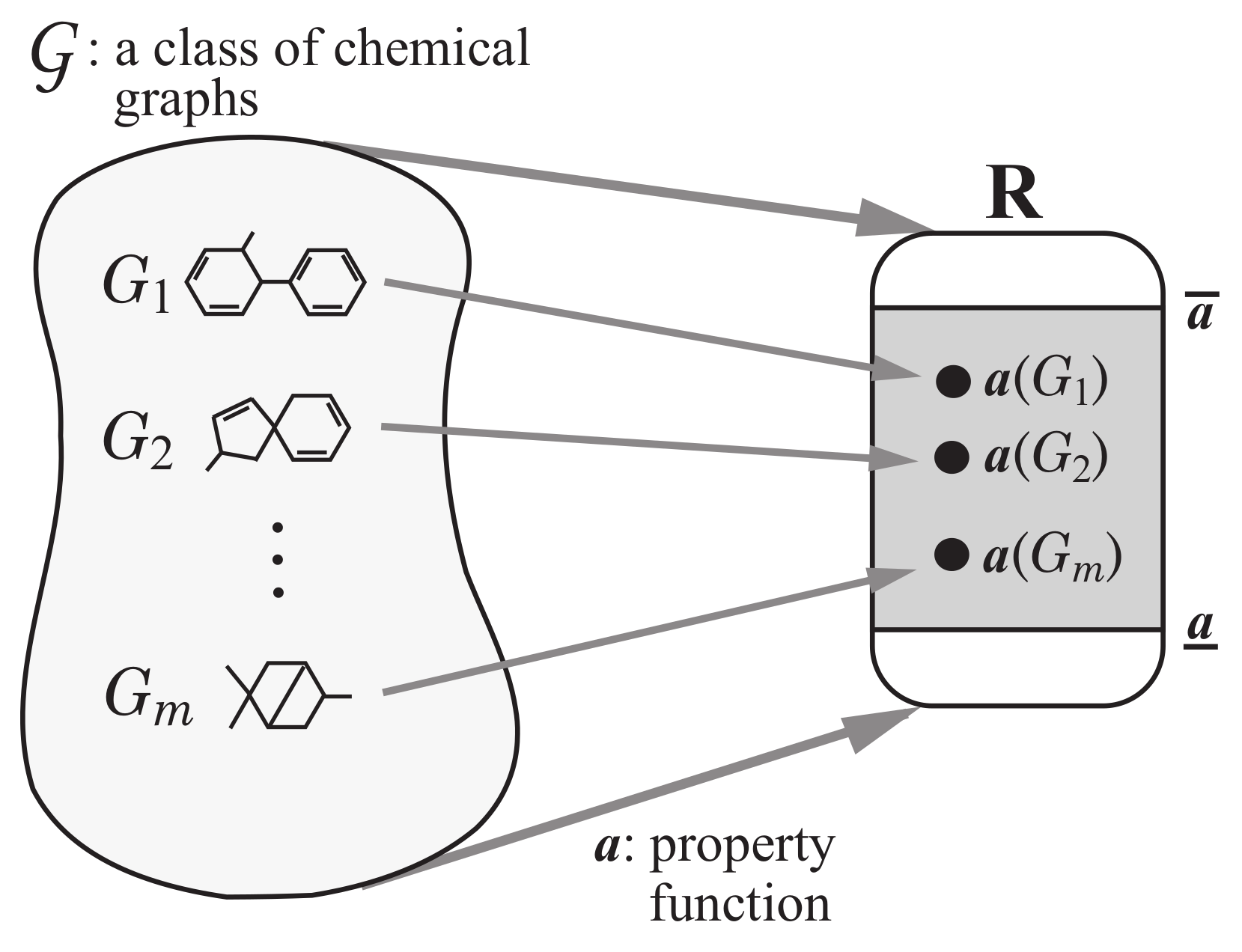
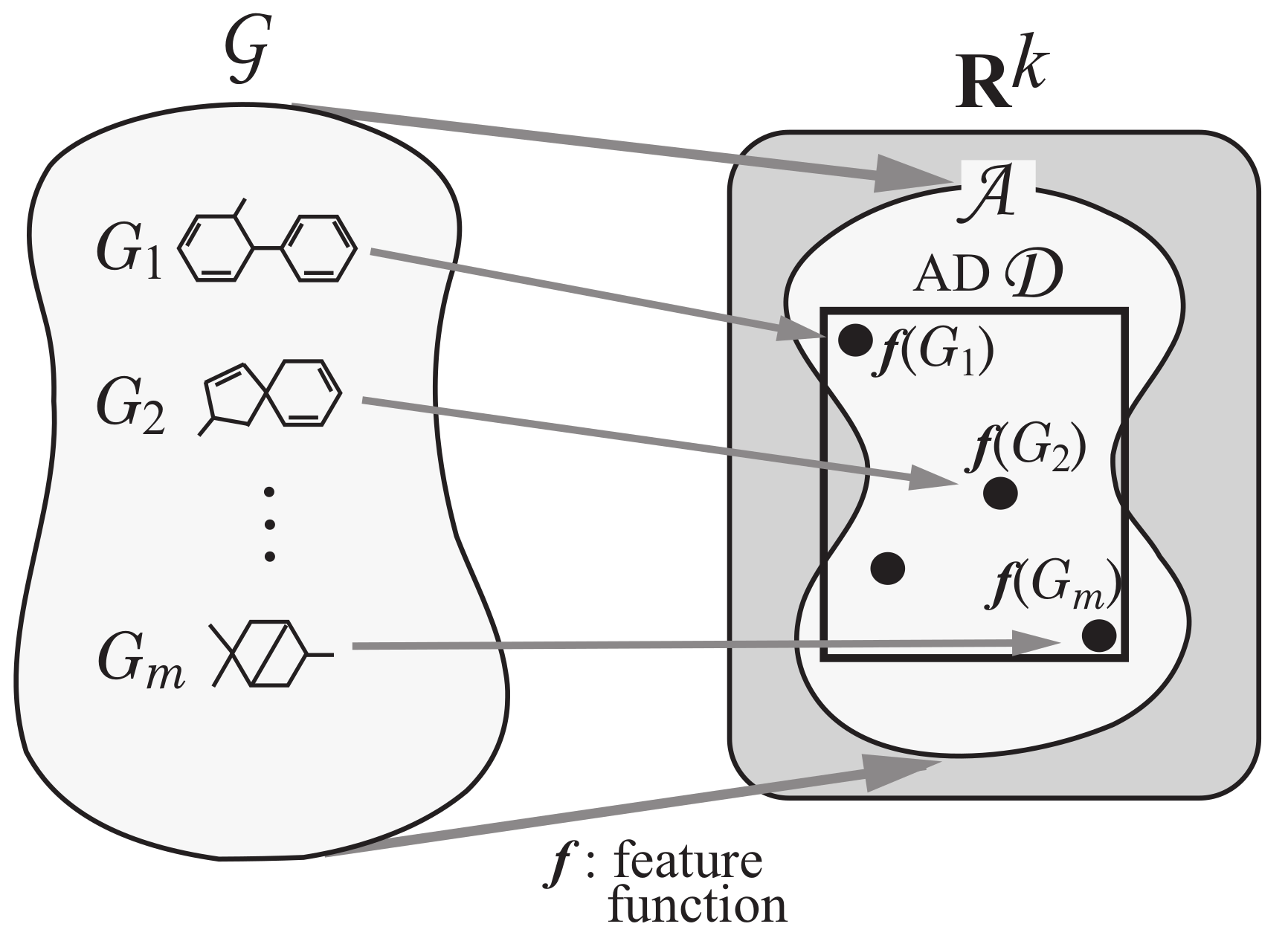
Appendix A.1. Applicability Domain

We use the range-based method to define an applicability domain for our method. For this, we find the range (the minimum and maximum) of each descriptor over all relevant chemical compounds and represent each range as a set of linear constraints in the constraint set ${\mathcal{C}}_1$ of our MILP formulation. Recall that $D_{\pi }$ stands for a set of chemical graphs used for constructing a prediction function. However, the number of examples in $D_{\pi }$ may not be large enough to capture a general feature on the structure of chemical graphs. For this, we also use some data set from the whole set $\mathrm{DB}$ of chemical graphs in a database. Let ${\mathrm{DB}}_{\mathcal{G}}^{\left(i\right)}$ denote the set of chemical graphs $G\in \mathrm{DB}\cap \mathcal{G}$ such that $n\left(G\right)=i$ for each integer $i\ge 1$. Formally the set of variables and constraints is given as follows.

AD constraints in ${\mathcal{C}}_1$:

constants:

Integers ${\mathrm{cs}}^{*}\ge 3$ and ${\mathrm{ch}}^{*}\ge 1$; An integer $d_{max}\in \{3,4\}$;

An integer $n^{*}\in [{\mathrm{cs}}^{*}+1,{\mathrm{cs}}^{*}·{(d_{max}-1)}^{{\mathrm{ch}}^{*}}]$;

variables for descriptors in x:

A real variable ${\kappa }_1\ge 0$: ${\kappa }_1$ represents ${\kappa }_1\left(H\right)$;

$\mathrm{dg}\left(i\right)\in [0,n^{*}]$$(i\in [1,4\left]\right)$: $\mathrm{dg}\left(i\right)$ represents the number of vertices of degree i in H;

$\mathrm{Mass}\in \mathbb{Z}$: $\mathrm{Mass}$ represents ${\sum }_{v\in V}{\mathrm{mass}}^{*}\left(\alpha \left(v\right)\right)$;

${\mathrm{ce}}^{\mathrm{co}}\left(\mathtt{a}\right)\in [0,n^{*}]$, $\mathtt{a}\in \Lambda$: ${\mathrm{ce}}^{\mathrm{co}}\left(\mathtt{a}\right)$ represents the number of vertices of chemical element

a in the core of H;

${\mathrm{ce}}^{\mathrm{nc}}\left(\mathtt{a}\right)\in [0,n^{*}]$, $\mathtt{a}\in \Lambda$: ${\mathrm{ce}}^{\mathrm{nc}}\left(\mathtt{a}\right)$ represents the number of vertices of chemical element

a in the non-core of H;

${\mathrm{b}}^{\mathrm{co}}\left(k\right)\in [0,2n^{*}]$, $k\in [1,3]$: ${\mathrm{b}}^{\mathrm{co}}\left(k\right)$ represents the number of k-bonds in the core of H;

${\mathrm{b}}^{\mathrm{nc}}\left(k\right)\in [0,2n^{*}]$, $k\in [1,3]$: ${\mathrm{b}}^{\mathrm{nc}}\left(k\right)$ represents the number of k-bonds in the non-core of H;

${\mathrm{ac}}^{\mathrm{co}}\left(\gamma \right)\in [0,n^{*}]$, $\gamma \in {\Gamma }_{<}\cup {\Gamma }_{=}$: ${\mathrm{ac}}^{\mathrm{co}}\left(\gamma \right)$ represents the number of core edges

in H that are assigned tuple $\gamma \in {\Gamma }_{<}$;

${\mathrm{ac}}^{\mathrm{nc}}\left(\gamma \right)\in [0,n^{*}]$, $\gamma \in {\Gamma }_{<}\cup {\Gamma }_{=}$: ${\mathrm{ac}}^{\mathrm{nc}}\left(\gamma \right)$ represents the number of non-core edges in

H that are assigned tuple $\gamma \in {\Gamma }_{<}$;

constraints:

$$\begin{array}{c}\hfill n^{*}\underset{G\in D_{\pi }\cup {\mathrm{DB}}_{\mathcal{G}}^{\left(n^{*}\right)}}{min}\frac{{\kappa }_1\left(G\right)}{n\left(G\right)}\le {\kappa }_1\le n^{*}\underset{G\in D_{\pi }\cup {\mathrm{DB}}_{\mathcal{G}}^{\left(n^{*}\right)}}{max}\frac{{\kappa }_1\left(G\right)}{n\left(G\right)},\end{array}$$

(A1)

$$\begin{array}{ccc}\hfill n^{*}\underset{G\in D_{\pi }\cup {\mathrm{DB}}_{\mathcal{G}}^{\left(n^{*}\right)}}{min}\frac{{\mathrm{dg}}_i\left(G\right)}{n\left(G\right)}\le \mathrm{dg}\left(i\right)\le n^{*}\underset{G\in D_{\pi }\cup {\mathrm{DB}}_{\mathcal{G}}^{\left(n^{*}\right)}}{max}\frac{{\mathrm{dg}}_i\left(G\right)}{n\left(G\right)},& \hfill & \hfill i\in [1,4],\end{array}$$

(A2)

$$\begin{array}{c}\hfill n^{*}\underset{G\in D_{\pi }\cup {\mathrm{DB}}_{\mathcal{G}}^{\left(n^{*}\right)}}{min}\overline{\mathrm{ms}}\left(G\right)\le \mathrm{Mass}\le n^{*}\underset{G\in D_{\pi }\cup {\mathrm{DB}}_{\mathcal{G}}^{\left(n^{*}\right)}}{max}\overline{\mathrm{ms}}\left(G\right),\end{array}$$

(A3)

$$\begin{array}{ccc}\hfill n^{*}\underset{G\in D_{\pi }\cup {\mathrm{DB}}_{\mathcal{G}}^{\left(n^{*}\right)}}{min}\frac{{\mathrm{ce}}_{\mathtt{a}}^{\mathrm{co}}\left(G\right)}{n\left(G\right)}\le {\mathrm{ce}}^{\mathrm{co}}\left(\mathtt{a}\right)\le n^{*}\underset{G\in D_{\pi }\cup {\mathrm{DB}}_{\mathcal{G}}^{\left(n^{*}\right)}}{max}\frac{{\mathrm{ce}}_{\mathtt{a}}^{\mathrm{co}}\left(G\right)}{n\left(G\right)},& \hfill & \hfill \mathtt{a}\in \Lambda ,\end{array}$$

(A4)

$$\begin{array}{ccc}\hfill n^{*}\underset{G\in D_{\pi }\cup {\mathrm{DB}}_{\mathcal{G}}^{\left(n^{*}\right)}}{min}\frac{{\mathrm{ce}}_{\mathtt{a}}^{\mathrm{nc}}\left(G\right)}{n\left(G\right)}\le {\mathrm{ce}}^{\mathrm{nc}}\left(\mathtt{a}\right)\le n^{*}\underset{G\in D_{\pi }\cup {\mathrm{DB}}_{\mathcal{G}}^{\left(n^{*}\right)}}{max}\frac{{\mathrm{ce}}_{\mathtt{a}}^{\mathrm{nc}}\left(G\right)}{n\left(G\right)},& \hfill & \hfill \mathtt{a}\in \Lambda ,\end{array}$$

(A5)

$$\begin{array}{ccc}\hfill (n^{*}+1)\underset{G\in D_{\pi }\cup {\mathrm{DB}}_{\mathcal{G}}^{\left(n^{*}\right)}}{min}\frac{b_k^{\mathrm{co}}\left(G\right)}{n\left(G\right)+1}\le {\mathrm{b}}^{\mathrm{co}}\left(k\right)\le (n^{*}+1)\underset{G\in D_{\pi }\cup {\mathrm{DB}}_{\mathcal{G}}^{\left(n^{*}\right)}}{max}\frac{b_k^{\mathrm{co}}\left(G\right)}{n\left(G\right)+1},& \hfill & \hfill k\in [2,3],\end{array}$$

(A6)

$$\begin{array}{ccc}\hfill (n^{*}+1)\underset{G\in D_{\pi }\cup {\mathrm{DB}}_{\mathcal{G}}^{\left(n^{*}\right)}}{min}\frac{b_k^{\mathrm{nc}}\left(G\right)}{n\left(G\right)+1}\le {\mathrm{b}}^{\mathrm{nc}}\left(k\right)\le (n^{*}+1)\underset{G\in D_{\pi }\cup {\mathrm{DB}}_{\mathcal{G}}^{\left(n^{*}\right)}}{max}\frac{b_k^{\mathrm{nc}}\left(G\right)}{n\left(G\right)+1},& \hfill & \hfill k\in [2,3],\end{array}$$

(A7)

$$\begin{array}{ccc}\hfill (n^{*}+1)\underset{G\in D_{\pi }\cup {\mathrm{DB}}_{\mathcal{G}}^{\left(n^{*}\right)}}{min}\frac{{\mathrm{ac}}_{\gamma }^{\mathrm{co}}\left(G\right)}{n\left(G\right)+1}\le {\mathrm{ac}}^{\mathrm{co}}\left(\gamma \right)\le (n^{*}+1)\underset{G\in D_{\pi }\cup {\mathrm{DB}}_{\mathcal{G}}^{\left(n^{*}\right)}}{max}\frac{{\mathrm{ac}}_{\gamma }^{\mathrm{co}}\left(G\right)}{n\left(G\right)+1},& \hfill & \hfill \gamma \in \Gamma ,\end{array}$$

(A8)

$$\begin{array}{ccc}\hfill (n^{*}+1)\underset{G\in D_{\pi }\cup {\mathrm{DB}}_{\mathcal{G}}^{\left(n^{*}\right)}}{min}\frac{{\mathrm{ac}}_{\gamma }^{\mathrm{nc}}\left(G\right)}{n\left(G\right)+1}\le {\mathrm{ac}}^{\mathrm{nc}}\left(\gamma \right)\le (n^{*}+1)\underset{G\in D_{\pi }\cup {\mathrm{DB}}_{\mathcal{G}}^{\left(n^{*}\right)}}{max}\frac{{\mathrm{ac}}_{\gamma }^{\mathrm{nc}}\left(G\right)}{n\left(G\right)+1},& \hfill & \hfill \gamma \in \Gamma .\end{array}$$

(A9)

In the following, we derive an MILP $\mathcal{M}(x,g;{\mathcal{C}}_2)$ that satisfies the condition in Theorem 2. Let $d_{max}\in \{3,4\}$, $n^{*}\ge 3$, ${\mathrm{cs}}^{*}\ge 3$ ${\mathrm{ch}}^{*}\ge 0$ and ${\theta }^{*}$ be given integers. We describe the set ${\mathcal{C}}_2$ with several sets of constraints.

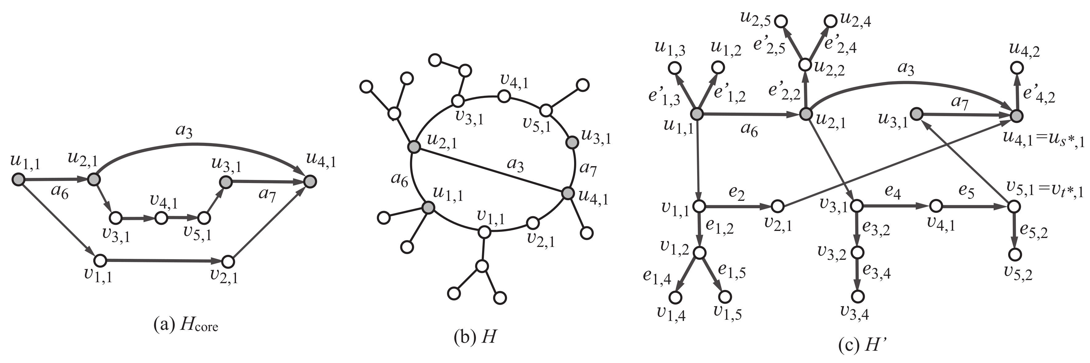
Appendix A.2. Construction of Scheme Graph and Tree-Extension

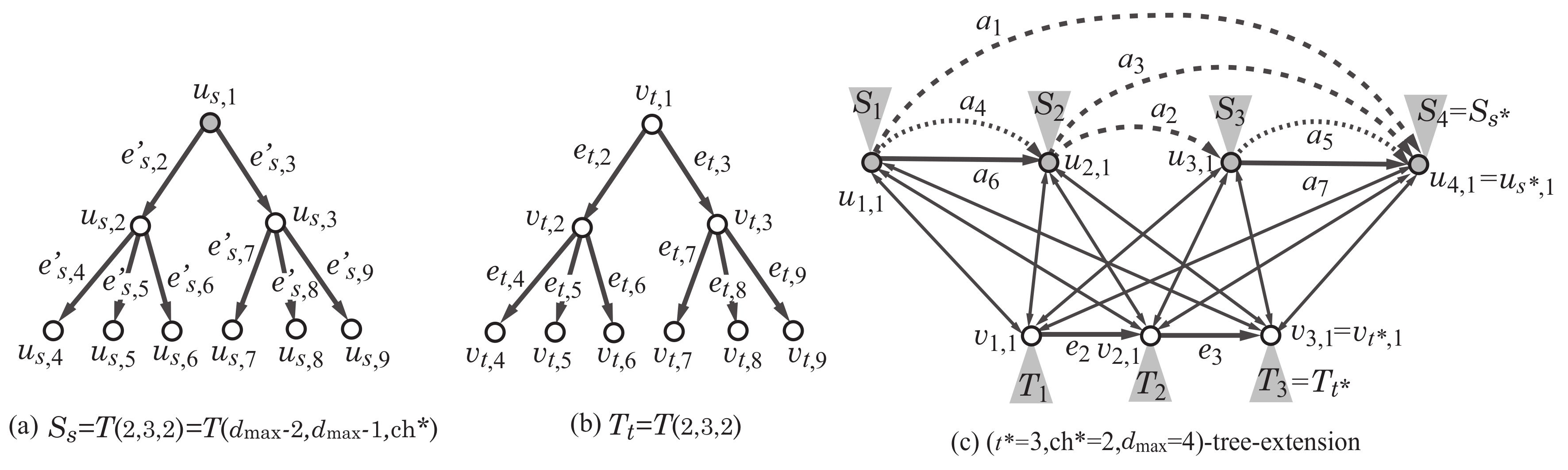
We infer a subgraph H such that the maximum degree is $d_{max}\in \{3,4\}$, $n\left(H\right)=n^{*}$, $\mathrm{cs}\left(H\right)={\mathrm{cs}}^{*}$ and $\mathrm{ch}\left(H\right)={\mathrm{ch}}^{*}$. For this, we first construct the $(t^{*},{\mathrm{ch}}^{*},d_{max})$-tree-extension of the scheme graph $(K=(V_K=\{u_1,\dots ,u_{s^{*}}\},E_K=\{a_1,a_2,\dots ,a_m\}),\mathcal{E}=(E_1,E_2,E_3))$. We use the following notations: For $j\in [1,3]$ and $s\in [1,s^{*}]$, let $E_j^{+}\left(s\right)$ (resp., $E_j^{-}\left(s\right)$) denote the set of indices i of edges $a_i\in E_i$ such that the tail (resp., head) of $a_i$ is $u_{s,1}$. Let $E_{j,k}^{+}\left(s\right)\triangleq E_j^{+}\left(s\right)\cup E_k^{+}\left(s\right)$, $E_{j,k}^{-}\left(s\right)\triangleq E_j^{-}\left(s\right)\cup E_k^{-}\left(s\right)$, $E_j\left(s\right)\triangleq E_j^{+}\left(s\right)\cup E_j^{-}\left(s\right)$ and $E_{j,k}\left(s\right)\triangleq E_j\left(s\right)\cup E_k\left(s\right)$.

As described in Section 2.3.1, some edge $a\left(i\right)\in E_1\cup E_2$ may be replaced with a subpath $P_i$ of $(v_{1,1},v_{1,2},\dots ,v_{t^{*},1})$, which consists of the roots of trees $T_1,T_2,\dots ,T_{t^{*}}$. We assign color i to the vertices in such a subpath $P_i$ by setting a variable $\chi \left(t\right)$ of each vertex $v_{t,1}\in V\left(P_i\right)$ to be i. For each edge $u_{s,1}{v}_{t,1}$, we prepare a binary variable $e(s,t)$ to denote that edge $u_{s,1}{v}_{t,1}$ is used (resp., not used) in a selected graph H when $e(s,t)=1$ (resp., $e(s,t)=0$). We also include constraints necessary for the variables to satisfy a degree condition at each of the vertices $u_{s,1}$, $s\in [1,s^{*}]$ and $v_{t,1}$, $t\in [1,t^{*}]$.

constants:

Integers $s^{*}=\left|V_K\right|$, $c^{*}=|E_1\cup E_2|$, ${\mathrm{cs}}^{*}(\ge s^{*})$, $n^{*}(\ge {\mathrm{cs}}^{*})$ and ${\mathrm{ch}}^{*}\ge 0$;

${\underline{d}}^{+}\left(s\right)$, $s\in [1,s^{*}]$: a lower bound on the out-degree of vertex $u_{s,1}$ in H;

${\underline{d}}^{-}\left(s\right)$, $s\in [1,s^{*}]$: a lower bound on the in-degree of vertex $u_{s,1}$ in H;

${\overline{d}}^{+}\left(s\right)$, $s\in [1,s^{*}]$: an upper bound on the out-degree of vertex $u_{s,1}$ in H;

${\overline{d}}^{-}\left(s\right)$, $s\in [1,s^{*}]$: an upper bound on the in-degree of vertex $u_{s,1}$ in H;

variables:

$a\left(i\right)\in \{0,1\}$, $i\in E_1\cup E_3$: $a\left(i\right)$ represents edge $a_i\in E_1\cup E_3$ ($a\left(i\right)=1$, $i\in E_1$)

($a\left(i\right)=1$ ⇔ edge $a_i$ is used in H);

$e(s,t),e(t,s)\in \{0,1\}$, $s\in [1,s^{*}]$, $t\in [1,t^{*}]$: $e(s,t)$ (resp., $e(t,s)$) represents

direction $(u_{s,1},v_{t,1})$ (resp., $(v_{t,1},u_{s,1})$), where $e(s,t)=1$ (resp., $e(t,s)=1$) ⇔

edge $u_{s,1},v_{t,1}$ is used in H and direction $(u_{s,1},v_{t,1})$ (resp., $(v_{t,1},u_{s,1})$) is assigned

to edge $u_{s,1},v_{t,1}$;

$\chi \left(t\right)\in [1,c^{*}]$, $t\in [1,t^{*}]$: $\chi \left(t\right)$ represents the color assigned to vertex $v_{t,1}$

($\chi \left(t\right)=c$ ⇔ vertex $v_{t,1}$ is assigned color c);

$\mathrm{clr}\left(c\right)\in [0,n^{*}-s^{*}]$, $c\in [1,c^{*}]$: the number of vertices $v_{t,i}$ with color c;

${\mathrm{deg}}^{\mathrm{co}}+\left(s\right)\in [1,4]$, $s\in [1,s^{*}]$: the out-degree of vertex $u_{s,1}$ in the core of H;

${\mathrm{deg}}^{\mathrm{co}}-\left(s\right)\in [1,4]$, $s\in [1,s^{*}]$: the in-degree of vertex $u_{s,1}$ in the core of H;

${\delta }_{\mathrm{clr}}(t,c)\in \{0,1\}$, $t\in [1,t^{*}]$, $c\in [1,c^{*}]$ (${\delta }_{\mathrm{clr}}(t,c)=1$ ⇔ $\chi \left(t\right)=c$);

constraints:

$$\begin{array}{ccc}\hfill \sum _{c\in [1,c^{*}]}{\delta }_{\mathrm{clr}}(t,c)=1,& \hfill & \hfill t\in [1,t^{*}],\end{array}$$

(A10)

$$\begin{array}{ccc}\hfill \sum _{c\in [1,c^{*}]}c·{\delta }_{\mathrm{clr}}(t,c)=\chi \left(t\right),& \hfill & \hfill t\in [1,t^{*}],\end{array}$$

(A11)

$$\begin{array}{ccc}\hfill \sum _{t\in [1,t^{*}]}{\delta }_{\mathrm{clr}}(t,c)=\mathrm{clr}\left(c\right),& \hfill & \hfill c\in [1,c^{*}],\end{array}$$

(A12)

$$\begin{array}{ccc}\hfill e(s,t)+e(t,s)\le 1,& \hfill & \hfill s\in [1,s^{*}],t\in [1,t^{*}],\end{array}$$

(A13)

$$\begin{array}{ccc}\hfill \sum _{s\in [1,s^{*}]\setminus \left\{\mathrm{head}\left(c\right)\right\}}e(t,s)\le 1-{\delta }_{\mathrm{clr}}(t,c),& \hfill & \hfill c\in [1,c^{*}],t\in [1,t^{*}],\end{array}$$

(A14)

$$\begin{array}{ccc}\hfill \sum _{s\in [1,s^{*}]\setminus \left\{\mathrm{tail}\left(c\right)\right\}}e(s,t)\le 1-{\delta }_{\mathrm{clr}}(t,c),& \hfill & \hfill c\in [1,c^{*}],t\in [1,t^{*}],\end{array}$$

(A15)

$$\begin{array}{ccc}\hfill \sum _{i\in E_{1,3}^{-}\left(s\right)}a\left(i\right)+\sum _{t\in [1,t^{*}]}e(t,s)={\mathrm{deg}}^{\mathrm{co}}-\left(s\right),& \hfill & \hfill s\in [1,s^{*}],\end{array}$$

(A16)

$$\begin{array}{ccc}\hfill \sum _{i\in E_{1,3}^{+}\left(s\right)}a\left(i\right)+\sum _{t\in [1,t^{*}]}e(s,t)={\mathrm{deg}}^{\mathrm{co}}+\left(s\right),& \hfill & \hfill s\in [1,s^{*}],\end{array}$$

(A17)

$$\begin{array}{ccc}\hfill {\underline{d}}^{+}\left(s\right)\le {\mathrm{deg}}^{\mathrm{co}}+\left(s\right)\le {\overline{d}}^{+}\left(s\right),& \hfill & \hfill s\in [1,s^{*}],\end{array}$$

(A18)

$$\begin{array}{ccc}\hfill {\underline{d}}^{-}\left(s\right)\le {\mathrm{deg}}^{\mathrm{co}}-\left(s\right)\le {\overline{d}}^{-}\left(s\right),& \hfill & \hfill s\in [1,s^{*}].\end{array}$$

(A19)

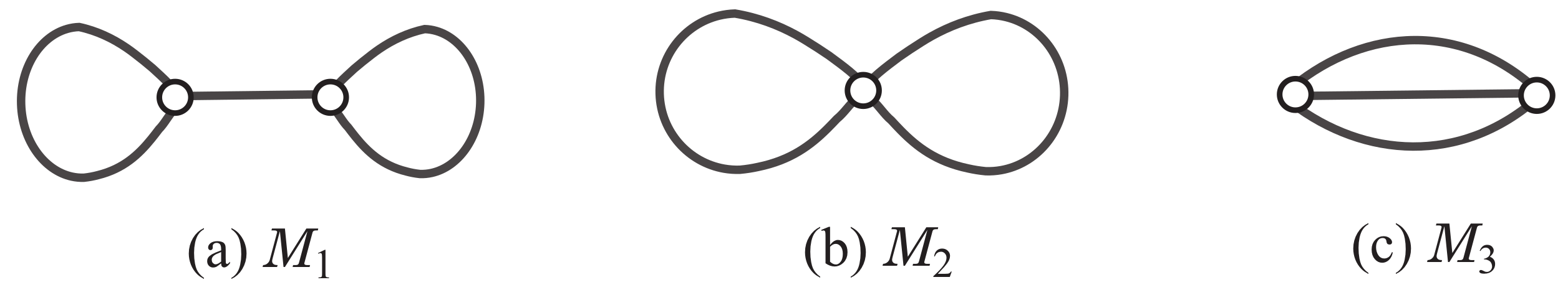
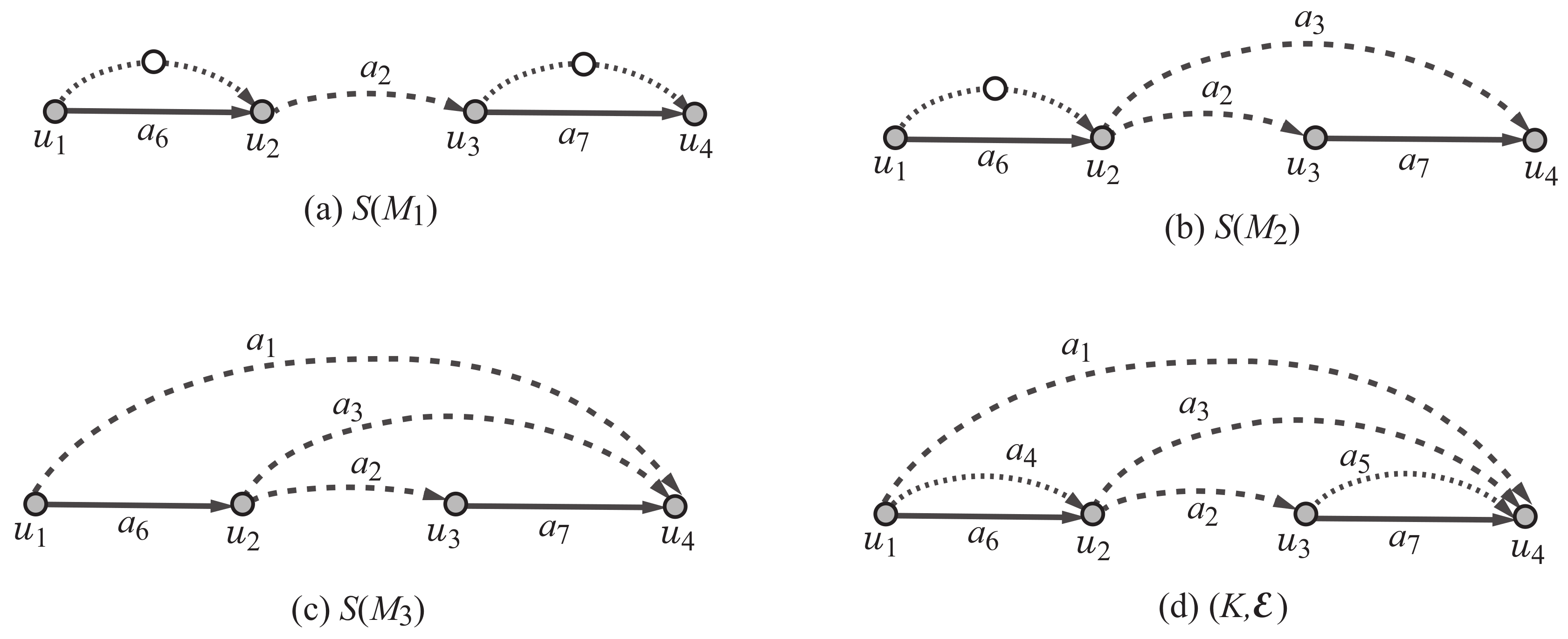
Appendix A.3. Specification for Chemical Graphs with Rank 2

To generate any of the three rank-2 polymer topologies in $\mathcal{PT}(2,4)$, we use the scheme graph $(K=(V_K=\{u_1,u_2,u_3,u_4\},E_K)$, $\mathcal{E}=(E_1,E_2,E_3))$ in Figure 2d, where $s^{*}=\left|V\left(K\right)\right|=4$, $c^{*}=|E_1\cup E_2|=5$, $E_1=\{a_1=(u_1,u_4),a_2=(u_2,u_3),a_3=(u_2,u_4)\}$, $E_2=\{a_4=(u_1,u_2),a_5=(u_3,u_4)\}$ and $E_3=\{a_6=(u_1,u_2),a_7=(u_3,u_4)\}$. Recall that each color $i\in [1,c^{*}]$ is assigned to edge $a_i\in E_1\cup E_2$. We impose some more constraints on the degree of each of the vertices $u_{s,1}$, $s\in [1,s^{*}]$ and $v_{t,1}$, $t\in [1,t^{*}]$ so that the core of a selected graph H satisfies one of the three least simple graphs in Figure 2a–c. We also let a variable $\theta$ mean the topological parameter $\theta \left(H\right)$ of a selected subgraph H.

constants:

$s^{*}=4$, $c^{*}=5$,

$E_1^{-}\left(1\right)=\varnothing$, $E_2^{-}\left(1\right)=\varnothing$, $E_3^{-}\left(1\right)=\varnothing$, $E_1^{+}\left(1\right)=\left\{1\right\}$, $E_2^{+}\left(1\right)=\left\{4\right\}$, $E_3^{+}\left(1\right)=\left\{6\right\}$,

$E_1^{-}\left(2\right)=\varnothing$, $E_2^{-}\left(2\right)=\left\{4\right\}$, $E_3^{-}\left(2\right)=\left\{6\right\}$, $E_1^{+}\left(2\right)=\{2,3\}$, $E_2^{+}\left(2\right)=\varnothing$, $E_3^{+}\left(2\right)=\varnothing$,

$E_1^{-}\left(3\right)=\left\{2\right\}$, $E_2^{-}\left(3\right)=\varnothing$, $E_3^{-}\left(3\right)=\varnothing$, $E_1^{+}\left(3\right)=\varnothing$, $E_2^{+}\left(3\right)=\left\{5\right\}$, $E_3^{+}\left(3\right)=\left\{7\right\}$,

$E_1^{-}\left(4\right)=\{1,3\}$, $E_2^{-}\left(4\right)=\left\{5\right\}$, $E_3^{-}\left(4\right)=\left\{7\right\}$, $E_1^{+}\left(4\right)=\varnothing$, $E_2^{+}\left(4\right)=\varnothing$, $E_3^{+}\left(4\right)=\varnothing$,

${\underline{d}}^{-}\left(1\right)=0$, ${\overline{d}}^{-}\left(1\right)=0$, ${\underline{d}}^{+}\left(1\right)=2$, ${\overline{d}}^{+}\left(1\right)=2$,

${\underline{d}}^{-}\left(2\right)=1$, ${\overline{d}}^{-}\left(2\right)=2$, ${\underline{d}}^{+}\left(2\right)=1$, ${\overline{d}}^{+}\left(2\right)=2$,

${\underline{d}}^{-}\left(3\right)=1$, ${\overline{d}}^{-}\left(3\right)=1$, ${\underline{d}}^{+}\left(3\right)=1$, ${\overline{d}}^{+}\left(3\right)=2$,

${\underline{d}}^{-}\left(4\right)=2$, ${\overline{d}}^{-}\left(4\right)=3$, ${\underline{d}}^{+}\left(4\right)=0$, ${\overline{d}}^{+}\left(4\right)=0$,

variables:

$\theta \in [-n^{*},n^{*}]$: The topology-parameter $\theta \left(H\right)$ for rank 2;

constraints:

$$\begin{array}{cc}\hfill a\left(2\right)+\mathrm{clr}\left(2\right)& \ge 1,\hfill \end{array}$$

(A20)

$$\begin{array}{cc}\hfill a\left(3\right)+\mathrm{clr}\left(3\right)+\mathrm{clr}\left(4\right)& \ge 1,\hfill \end{array}$$

(A21)

$$\begin{array}{cc}\hfill \mathrm{clr}\left(4\right)& \ge \mathrm{clr}\left(5\right),\hfill \end{array}$$

(A22)

$$\begin{array}{cc}\hfill \mathrm{clr}\left(3\right)& \le \mathrm{clr}\left(2\right)+1,\hfill \end{array}$$

(A23)

$$\begin{array}{cc}\hfill \mathrm{clr}\left(3\right)& \le \mathrm{clr}\left(1\right)+1+n^{*}(3-{\mathrm{deg}}^{\mathrm{co}-}\left(4\right)),\hfill \end{array}$$

(A24)

$$\begin{array}{cc}\hfill -\theta & \le 1+\mathrm{clr}\left(2\right)+n^{*}(2-{\mathrm{deg}}^{\mathrm{co}}+\left(3\right)),\hfill \end{array}$$

(A25)

$$\begin{array}{cc}\hfill -\theta & \ge 1+\mathrm{clr}\left(2\right)-n^{*}(2-{\mathrm{deg}}^{\mathrm{co}}+\left(3\right)),\hfill \end{array}$$

(A26)

$$\begin{array}{cc}\hfill \theta & \le n^{*}(4-{\mathrm{deg}}^{\mathrm{co}}+\left(2\right)-{\mathrm{deg}}^{\mathrm{co}}-\left(2\right)),\hfill \end{array}$$

(A27)

$$\begin{array}{cc}\hfill \theta & \ge -n^{*}(4-{\mathrm{deg}}^{\mathrm{co}}+\left(2\right)-{\mathrm{deg}}^{\mathrm{co}}-\left(2\right)),\hfill \end{array}$$

(A28)

$$\begin{array}{cc}\hfill \theta & \le 1+\mathrm{clr}\left(3\right)+n^{*}(3-{\mathrm{deg}}^{\mathrm{co}}-\left(4\right)),\hfill \end{array}$$

(A29)

$$\begin{array}{cc}\hfill \theta & \ge 1+\mathrm{clr}\left(3\right)-n^{*}(3-{\mathrm{deg}}^{\mathrm{co}}-\left(4\right)).\hfill \end{array}$$

(A30)

Appendix A.4. Selecting A Subgraph

We prepare a binary variable $u(s,i)$ (resp., $v(t,i)$) for each vertex $u_{s,i}$ in tree $S_s$ (resp., $v_{t,i}$ in tree $T_t$). We include constraints so that the path $(v_{1,1},v_{1,2},\dots ,v_{t^{*},1})$ is partitioned into subpaths $P_c$, $c\in [1,c^{*}]$, where possibly some $P_c$ is empty, and the resulting subgraph H becomes a connected rank-2 graph with $n\left(H\right)=n^{*}$, $\mathrm{cs}\left(H\right)={\mathrm{cs}}^{*}$, $\mathrm{ch}\left(H\right)={\mathrm{ch}}^{*}$ and $\theta \left(H\right)={\theta }^{*}$.

constants:

Integers $d_{max}\in \{3,4\}$, ${\mathrm{ch}}^{*}\ge 0$;

Prepare the set $\mathrm{Cld}\left(i\right)$ of the indices of children of a vertex $v_i$

the index $\mathrm{prt}\left(i\right)$ of the parent of a non-root vertex $v_i$, and

the set $\mathrm{Dst}\left(h\right)$ of indices i such that the height of a vertex $v_i$ is h

in the rooted tree $T(2,d_{max}-1,{\mathrm{ch}}^{*})$;

variables:

$u(s,i)\in \{0,1\}$, $s\in [1,s^{*}]$, $i\in [1,n_{\mathrm{tree}}]$: $u(s,i)$ represents vertex $u_{s,i}$

($u(s,i)=1$ ⇔ vertex $u_{s,i}$ is used in H and edge $e_{s,i}^{\prime }$ $(i\ge 2)$ is used in H);

$v(t,i)\in \{0,1\}$, $t\in [1,t^{*}]$, $i\in [1,n_{\mathrm{tree}}]$: $v(t,i)$ represents vertex $v_{t,i}$

($v(t,i)=1$ ⇔ vertex $v_{t,i}$ is used in H and edge $e_{t,i}$$(i\ge 2)$ is used in H);

$e\left(t\right)\in \{0,1\}$, $t\in [1,t^{*}+1]$: $e\left(t\right)$ represents edge $e_t=v_{t-1,1}{v}_{t,i}$,

where $e_{1,1}$ and $e_{t^{*}+1,1}$ are fictitious edges ($e\left(t\right)=1$ ⇔ edge $e_t$ is used in H);

constraints:

$$\begin{array}{ccc}\hfill u(s,1)=1,& \hfill & \hfill s\in [1,s^{*}],\end{array}$$

(A31)

$$\begin{array}{ccc}\hfill d_{max}·u(t,i)\ge \sum _{j\in \mathrm{Cld}\left(i\right)}u(t,j),& \hfill & \hfill t\in [1,{\mathrm{cs}}^{*}],i\in [2,n_{\mathrm{in}}],\end{array}$$

(A32)

$$\begin{array}{ccc}\hfill v(t,1)=1,& \hfill & \hfill t\in [1,t^{*}],\end{array}$$

(A33)

$$\begin{array}{ccc}\hfill d_{max}·v(t,i)\ge \sum _{j\in \mathrm{Cld}\left(i\right)}v(t,j),& \hfill & \hfill t\in [1,{\mathrm{cs}}^{*}],i\in [2,n_{\mathrm{in}}],\end{array}$$

(A34)

$$\begin{array}{c}\hfill \sum _{s\in [1,s^{*}],i\in [1,n_{\mathrm{tree}}]}u(s,i)+\sum _{t\in [1,t^{*}],i\in [1,n_{\mathrm{tree}}]}v(t,i)=n^{*},\end{array}$$

(A35)

$$\begin{array}{c}\hfill \sum _{s\in [1,s^{*}],i\in \mathrm{Dst}\left({\mathrm{ch}}^{*}\right)}u(s,i)+\sum _{t\in [1,t^{*}],i\in \mathrm{Dst}\left({\mathrm{ch}}^{*}\right)}v(t,i)\ge 1,\end{array}$$

(A36)

$$\begin{array}{c}\hfill e\left(1\right)=e(t^{*}+1)=0,\end{array}$$

(A37)

$$\begin{array}{ccc}\hfill e(t+1)+\sum _{s\in [1,s^{*}]}e(t,s)=1,& \hfill & \hfill t\in [1,t^{*}],\end{array}$$

(A38)

$$\begin{array}{ccc}\hfill e\left(t\right)+\sum _{s\in [1,s^{*}]}e(s,t)=1,& \hfill & \hfill t\in [1,t^{*}],\end{array}$$

(A39)

$$\begin{array}{c}\hfill c^{*}\ge \chi \left(1\right)\ge \chi \left(2\right)\ge \cdots \ge \chi \left(t^{*}\right)\ge 1,\end{array}$$

(A40)

$$\begin{array}{ccc}\hfill e(t+1)\ge 1+\chi (t+1)-\chi \left(t\right),& \hfill & \hfill t\in [1,t^{*}-1],\end{array}$$

(A41)

$$\begin{array}{ccc}\hfill c^{*}·(1-e(t+1))\ge \chi \left(t\right)-\chi (t+1),& \hfill & \hfill t\in [1,t^{*}-1].\end{array}$$

(A42)

Appendix A.5. Assigning Multiplicity

We prepare an integer variable $\tilde{\beta }\left(e\right)$ or $\widehat{\beta }\left(e\right)$ for each edge e in the $(t^{*},{\mathrm{ch}}^{*},d_{max})$-tree-extension of the scheme graph to denote the multiplicity of e in a selected graph H and include necessary constraints for the variables to satisfy in H.

variables:

$\tilde{\beta }\left(i\right)\in [0,3]$, $i\in E_1\cup E_3$: $\tilde{\beta }\left(i\right)$ represents the multiplicity of edge $a_i$,

where $\tilde{\beta }\left(i\right)=0$ if edge $a_i$ is not in H;

$\tilde{\beta }(p,i)\in [0,3]$, $p\in [1,{\mathrm{cs}}^{*}]$, $i\in [2,n_{\mathrm{tree}}]$: $\tilde{\beta }(p,i)$ with $p\le s^{*}$ (resp., $p>s^{*}$) represents

the multiplicity of edge $e_{p,i}^{\prime }$ (resp., $e_{p-s^{*},i}$);

$\tilde{\beta }(t,1)\in [0,3]$, $t\in [1,t^{*}+1]$: $\tilde{\beta }(t,1)$ represents the multiplicity of edge $e_t$;

$\widehat{\beta }(s,t)\in [0,3]$, $s\in [1,s^{*}]$, $t\in [1,t^{*}]$: $\widehat{\beta }(s,t)$ represents the multiplicity of edge $u_{s,1}{v}_{t,1}$;

constraints:

$$\begin{array}{ccc}\hfill a\left(i\right)=1,& \hfill & \hfill i\in E_3,\end{array}$$

(A43)

$$\begin{array}{ccc}\hfill a\left(i\right)\le \tilde{\beta }\left(i\right)\le 3a\left(i\right),& \hfill & \hfill i\in E_1\cup E_3,\end{array}$$

(A44)

$$\begin{array}{ccc}\hfill u(s,i)\le \tilde{\beta }(s,i)\le 3u(s,i),& \hfill & \hfill s\in [1,s^{*}],i\in [2,n_{\mathrm{tree}}],\end{array}$$

(A45)

$$\begin{array}{ccc}\hfill v(t,i)\le \tilde{\beta }(s^{*}+t,i)\le 3v(t,i),& \hfill & \hfill t\in [1,t^{*}],i\in [2,n_{\mathrm{tree}}],\end{array}$$

(A46)

$$\begin{array}{ccc}\hfill e\left(t\right)\le \tilde{\beta }(t,1)\le 3e\left(t\right),& \hfill & \hfill t\in [1,t^{*}+1],\end{array}$$

(A47)

$$\begin{array}{ccc}\hfill e(s,t)+e(t,s)\le \widehat{\beta }(s,t)\le 3e(s,t)+3e(t,s),& \hfill & \hfill s\in [1,s^{*}],t\in [1,t^{*}].\end{array}$$

(A48)

Appendix A.6. Assigning Chemical Elements and Valence Condition

We include constraints so that each vertex v in a selected graph H satisfies the valence condition; i.e., ${\sum }_{uv\in E\left(H\right)}\beta \left(uv\right)\le \mathrm{val}\left(\alpha \left(u\right)\right)$. With these constraints, a rank-2 chemical graph $G=(H,\alpha ,\beta )$ on a selected subgraph H will be constructed.

constants:

A set $\Lambda \cup \left\{ϵ\right\}$ of chemical elements, where $ϵ$ denotes null;

A coding $\left[\mathtt{a}\right]$, $\mathtt{a}\in \Lambda \cup \left\{ϵ\right\}$ such that $\left[ϵ\right]=0$; $\left[\mathtt{a}\right]\ge 1$, $\mathtt{a}\in \Lambda$; and $\left[\mathtt{a}\right]\ne \left[\mathtt{b}\right]$ if $\mathtt{a}\ne \mathtt{b}$;

Let $[\Lambda ]$ and $[\Lambda \cup \{ϵ\left\}\right]$ denote $\left\{\right[\mathtt{a}]\mid \mathtt{a}\in \Lambda \}$ and $\left\{\right[\mathtt{a}]\mid \mathtt{a}\in \Lambda \cup \{ϵ\left\}\right\}$, respectively;

A valence function: $\mathrm{val}:\Lambda \to [1,4]$;

variables:

$\tilde{\alpha }(p,i)\in [\Lambda \cup \left\{ϵ\right\}]$, $p\in [1,{\mathrm{cs}}^{*}]$, $i\in [1,n_{\mathrm{tree}}]$:

$\tilde{\alpha }(p,i)$ with $p\le s^{*}$ (resp., $p>s^{*}$) represents $\alpha \left(u_{p,i}\right)$ (resp., $\alpha \left(v_{p-s^{*},i}\right)$);

${\delta }_{\alpha }(p,i,\mathtt{a})\in \{0,1\}$, $p\in [1,{\mathrm{cs}}^{*}]$, $i\in [1,n_{\mathrm{tree}}]$, $\mathtt{a}\in \Lambda \cup \left\{ϵ\right\}$:

${\delta }_{\alpha }(p,i,\mathtt{a})=1$ ⇔ $\alpha \left(u_{p,i}\right)=\mathtt{a}$ for $p\le s^{*}$ and $\alpha \left(v_{p-s^{*},i}\right)=\mathtt{a}$ for $p>s^{*}$;

${\delta }_{\tilde{\beta }}(i,k)\in \{0,1\}$, $p\in [1,{\mathrm{cs}}^{*}]$, $i\in E_1\cup E_3$, $k\in [0,3]$:

${\delta }_{\tilde{\beta }}(i,k)=1$ ⇔ the multiplicity of edge $a_i$ in H is k;

${\delta }_{\tilde{\beta }}(p,i,k)\in \{0,1\}$, $p\in [1,{\mathrm{cs}}^{*}]$, $i\in [2,n_{\mathrm{tree}}]$, $k\in [0,3]$:

${\delta }_{\tilde{\beta }}(p,i,k)=1$ ⇔ the multiplicity of edge $e_{p,i}^{\prime }$, $p\le s^{*}$ (or $e_{p-s^{*},i}$, $p>s^{*}$) in H is k;

${\delta }_{\tilde{\beta }}(t,1,k)\in \{0,1\}$, $t\in [1,t^{*}+1]$, $k\in [0,3]$:

${\delta }_{\tilde{\beta }}(t,1,k)=1$ ⇔ the multiplicity of edge $e_t$ in H is k;

${\delta }_{\widehat{\beta }}(s,t,k)\in \{0,1\}$, $s\in [1,s^{*}]$, $t\in [1,t^{*}]$, $k\in [0,3]$:

${\delta }_{\widehat{\beta }}(s,t,k)=1$ ⇔ the multiplicity of edge $u_{s,1}{v}_{t,1}$ in H is k;

constraints:

$$\begin{array}{ccc}\hfill \sum _{\mathtt{a}\in \Lambda \cup \left\{ϵ\right\}}{\delta }_{\alpha }(p,i,\mathtt{a})=1,& \hfill & \hfill p\in [1,{\mathrm{cs}}^{*}],i\in [1,n_{\mathrm{tree}}],\end{array}$$

(A49)

$$\begin{array}{ccc}\hfill \sum _{\mathtt{a}\in \Lambda \cup \left\{ϵ\right\}}\left[\mathtt{a}\right]·{\delta }_{\alpha }(p,i,\mathtt{a})=\tilde{\alpha }(p,i),& \hfill & \hfill p\in [1,{\mathrm{cs}}^{*}],i\in [1,n_{\mathrm{tree}}],\end{array}$$

(A50)

$$\begin{array}{ccc}\hfill \sum _{k\in [0,3]}{\delta }_{\tilde{\beta }}(i,k)=1,& \hfill & \hfill i\in E_1\cup E_3,\end{array}$$

(A51)

$$\begin{array}{ccc}\hfill \sum _{k\in [1,3]}k·{\delta }_{\tilde{\beta }}(i,k)=\tilde{\beta }\left(i\right),& \hfill & \hfill i\in E_1\cup E_3,\end{array}$$

(A52)

$$\begin{array}{ccc}\hfill \sum _{k\in [0,3]}{\delta }_{\tilde{\beta }}(p,i,k)=1,& \hfill & \hfill p\in [1,{\mathrm{cs}}^{*}],i\in [2,n_{\mathrm{tree}}],\end{array}$$

(A53)

$$\begin{array}{ccc}\hfill \sum _{k\in [1,3]}k·{\delta }_{\tilde{\beta }}(p,i,k)=\tilde{\beta }(p,i),& \hfill & \hfill p\in [1,{\mathrm{cs}}^{*}],i\in [2,n_{\mathrm{tree}}],\end{array}$$

(A54)

$$\begin{array}{ccc}\hfill \sum _{k\in [0,3]}{\delta }_{\tilde{\beta }}(t,1,k)=1,& \hfill & \hfill t\in [1,t^{*}+1],\end{array}$$

(A55)

$$\begin{array}{ccc}\hfill \sum _{k\in [1,3]}k·{\delta }_{\tilde{\beta }}(t,1,k)=\tilde{\beta }(t,1),& \hfill & \hfill t\in [1,t^{*}+1],\end{array}$$

(A56)

$$\begin{array}{ccc}\hfill \sum _{k\in [0,3]}{\delta }_{\widehat{\beta }}(s,t,k)=1,& \hfill & \hfill s\in [1,s^{*}],t\in [1,t^{*}],\end{array}$$

(A57)

$$\begin{array}{ccc}\hfill \sum _{k\in [0,3]}k{\delta }_{\widehat{\beta }}(s,t,k)=\widehat{\beta }(s,t),& \hfill & \hfill s\in [1,s^{*}],t\in [1,t^{*}],\end{array}$$

(A58)

$$\begin{array}{c}\hfill \sum _{i\in E_{1,3}\left(s\right)}\tilde{\beta }\left(i\right)+\sum _{t\in [1,t^{*}]}\widehat{\beta }(s,t)\end{array}$$

$$\begin{array}{ccc}\hfill +\sum _{j\in \mathrm{Cld}\left(1\right)}\tilde{\beta }(s,j)\le \sum _{\mathtt{a}\in \Lambda }\mathrm{val}\left(\mathtt{a}\right)·{\delta }_{\alpha }(s,1,\mathtt{a}),& \hfill & \hfill s\in [1,s^{*}],\\ \hfill \sum _{s\in [1,s^{*}]}\widehat{\beta }(s,t)+\tilde{\beta }(t,1)+\tilde{\beta }(t+1,1)\end{array}$$

(A59)

$$\begin{array}{ccc}\hfill +\sum _{j\in \mathrm{Cld}\left(1\right)}\tilde{\beta }(s^{*}+t,j)\le \sum _{\mathtt{a}\in \Lambda }\mathrm{val}\left(\mathtt{a}\right)·{\delta }_{\alpha }(s^{*}+t,1,\mathtt{a}),& \hfill & \hfill t\in [1,t^{*}],\end{array}$$

(A60)

$$\begin{array}{ccc}\hfill \tilde{\beta }(p,i)+\sum _{j\in \mathrm{Cld}\left(i\right)}\tilde{\beta }(p,j)\le \sum _{\mathtt{a}\in \Lambda }\mathrm{val}\left(\mathtt{a}\right)·{\delta }_{\alpha }(p,i,\mathtt{a}),& \hfill & \hfill p\in [1,{\mathrm{cs}}^{*}],i\in [2,n_{\mathrm{tree}}].\end{array}$$

(A61)

Appendix A.7. Descriptors for Mass, the Numbers of Elements and Bonds

We include constraints to compute descriptors $\overline{\mathrm{ms}}\left(G\right)$ ${\mathrm{ce}}_{\mathtt{a}}^{\mathrm{co}}\left(G\right)$, ${\mathrm{ce}}_{\mathtt{a}}^{\mathrm{nc}}\left(G\right)$ ($\mathtt{a}\in \Lambda )$, $b_k\left(G\right)$ ($k\in [2,3]$) and $n_{\mathtt{H}}\left(G\right)$ according to the definitions in Section 2.1.2.

constants:

A function ${\mathrm{mass}}^{*}:\Lambda \to \mathbb{Z}$; Let $\mathrm{mass}\left(\mathtt{a}\right)$ denote the observed mass of a chemical element $\mathtt{a}\in \Lambda$, and

define ${\mathrm{mass}}^{*}\left(\mathtt{a}\right)=\lfloor 10·\mathrm{mass}\left(\mathtt{a}\right)\rfloor$;

variables:

${\mathrm{ce}}^{\mathrm{co}}\left(\mathtt{a}\right)\in [0,n^{*}]$, $\mathtt{a}\in \Lambda$;

${\mathrm{ce}}^{\mathrm{nc}}\left(\mathtt{a}\right)\in [0,n^{*}]$, $\mathtt{a}\in \Lambda$;

$\mathrm{Mass}\in \mathbb{Z}$;

${\mathrm{b}}^{\mathrm{co}}\left(k\right)\in [0,2n^{*}]$, $k\in [1,3]$;

${\mathrm{b}}^{\mathrm{nc}}\left(k\right)\in [0,2n^{*}]$, $k\in [1,3]$;

${\mathrm{n}}_{\mathtt{H}}\in [0,4n^{*}]$: the number of hydrogen atoms to be included in G;

constraints:

$$\begin{array}{ccc}\hfill \sum _{p\in [1,{\mathrm{cs}}^{*}]}{\delta }_{\alpha }(p,1,\mathtt{a})={\mathrm{ce}}^{\mathrm{co}}\left(\mathtt{a}\right),& \hfill & \hfill \mathtt{a}\in \Lambda ,\end{array}$$

(A62)

$$\begin{array}{ccc}\hfill \sum _{p\in [1,{\mathrm{cs}}^{*}],i\in [2,n_{\mathrm{tree}}]}{\delta }_{\alpha }(p,i,\mathtt{a})={\mathrm{ce}}^{\mathrm{nc}}\left(\mathtt{a}\right),& \hfill & \hfill \mathtt{a}\in \Lambda ,\end{array}$$

(A63)

$$\begin{array}{ccc}\hfill \sum _{\mathtt{a}\in \Lambda }{\mathrm{mass}}^{*}\left(\mathtt{a}\right)({\mathrm{ce}}^{\mathrm{co}}\left(\mathtt{a}\right)+{\mathrm{ce}}^{\mathrm{nc}}\left(\mathtt{a}\right))=\mathrm{Mass},& \hfill & \hfill \\ \hfill \sum _{i\in E_1\cup E_3}{\delta }_{\tilde{\beta }}(i,k)+\sum _{s\in [1,s^{*}],t\in [1,t^{*}]}{\delta }_{\widehat{\beta }}(s,t,k)& \hfill & \hfill \end{array}$$

(A64)

$$\begin{array}{ccc}\hfill +\sum _{t\in [2,t^{*}]}{\delta }_{\tilde{\beta }}(t,1,k)={\mathrm{b}}^{\mathrm{co}}\left(k\right),& \hfill & \hfill k\in [1,3],\end{array}$$

(A65)

$$\begin{array}{ccc}\hfill \sum _{p\in [1,{\mathrm{cs}}^{*}],i\in [2,n_{\mathrm{tree}}]}{\delta }_{\tilde{\beta }}(p,i,k)={\mathrm{b}}^{\mathrm{nc}}\left(k\right),& \hfill & \hfill k\in [1,3],\\ \hfill \sum _{\mathtt{a}\in \Lambda }\mathrm{val}\left(\mathtt{a}\right)({\mathrm{ce}}^{\mathrm{co}}\left(\mathtt{a}\right)+{\mathrm{ce}}^{\mathrm{nc}}\left(\mathtt{a}\right))\end{array}$$

(A66)

$$\begin{array}{c}\hfill -2(n^{*}+1+{\mathrm{b}}^{\mathrm{co}}\left(2\right)+{\mathrm{b}}^{\mathrm{nc}}\left(2\right)+2{\mathrm{b}}^{\mathrm{co}}\left(3\right)+2{\mathrm{b}}^{\mathrm{nc}}\left(3\right))={\mathrm{n}}_{\mathtt{H}}.\end{array}$$

(A67)

Appendix A.8. Descriptor for the Number of Specified Degree

We include constraints to compute descriptors ${\mathrm{dg}}_i\left(G\right)$ ($i\in [1,4]$) according to the definitions in Section 2.1.2. We also add constraints so that the maximum degree of a non-core vertex in H is at most 3 (resp., equal to 4) when $d_{max}=3$ (resp., $d_{max}=4)$.

variables:

$\mathrm{deg}(p,i)\in [0,4]$, $p\in [1,{\mathrm{cs}}^{*}]$, $i\in [1,n_{\mathrm{tree}}]$:

$\mathrm{deg}(p,i)$ represents ${\mathrm{deg}}_H\left(u_{p,i}\right)$ for $p\le s^{*}$ or ${\mathrm{deg}}_H\left(v_{p-s^{*},i}\right)$ for $p>s^{*}$;

${\delta }_{\mathrm{deg}}(p,i,d)\in \{0,1\}$, $p\in [1,{\mathrm{cs}}^{*}]$, $i\in [1,n_{\mathrm{tree}}]$, $d\in [0,4]$:

${\delta }_{\mathrm{deg}}(p,i,d)=1$ ⇔ $\mathrm{deg}(p,i)=d$;

$\mathrm{dg}\left(d\right)\in [0,n^{*}]$, $d\in [1,4]$;

constraints:

$$\begin{array}{c}\hfill \sum _{i\in E_{1,3}\left(s\right)}a\left(i\right)\end{array}$$

$$\begin{array}{ccc}\hfill +\sum _{t\in [1,t^{*}]}(e(s,t)+e(t,s))+\sum _{j\in \mathrm{Cld}\left(1\right)}u(s,j)=\mathrm{deg}(s,1),& \hfill & \hfill s\in [1,s^{*}],\end{array}$$

(A68)

$$\begin{array}{ccc}\hfill u(s,i)+\sum _{j\in \mathrm{Cld}\left(i\right)}u(s,j)=\mathrm{deg}(s,i),& \hfill & \hfill s\in [1,s^{*}],i\in [2,n_{\mathrm{tree}}],\end{array}$$

(A69)

$$\begin{array}{ccc}\hfill 2+\sum _{j\in \mathrm{Cld}\left(1\right)}v(t,j)=\mathrm{deg}(s^{*}+t,1),& \hfill & \hfill t\in [1,t^{*}],\end{array}$$

(A70)

$$\begin{array}{ccc}\hfill v(t,i)+\sum _{j\in \mathrm{Cld}\left(i\right)}v(t,j)=\mathrm{deg}(s^{*}+t,i),& \hfill & \hfill t\in [1,t^{*}],i\in [2,n_{\mathrm{tree}}],\end{array}$$

(A71)

$$\begin{array}{ccc}\hfill \sum _{d\in [0,4]}{\delta }_{\mathrm{deg}}(p,i,d)=1,& \hfill & \hfill p\in [1,{\mathrm{cs}}^{*}],i\in [1,n_{\mathrm{tree}}],\end{array}$$

(A72)

$$\begin{array}{ccc}\hfill \sum _{d\in [1,4]}d·{\delta }_{\mathrm{deg}}(p,i,d)=\mathrm{deg}(p,i),& \hfill & \hfill p\in [1,{\mathrm{cs}}^{*}],i\in [1,n_{\mathrm{tree}}],\end{array}$$

(A73)

$$\begin{array}{ccc}\hfill \sum _{p\in [1,{\mathrm{cs}}^{*}],i\in [1,n_{\mathrm{tree}}]}{\delta }_{\mathrm{deg}}(p,i,d)=\mathrm{dg}\left(d\right),& \hfill & \hfill d\in [1,4],\end{array}$$

(A74)

$$\begin{array}{ccc}\hfill \sum _{p\in [1,{\mathrm{cs}}^{*}],i\in [2,n_{\mathrm{tree}}]}{\delta }_{\mathrm{deg}}(p,i,4)\ge 1(resp.,=0)& \hfill & \hfill when{d}_{max}=4(resp.,=3).\end{array}$$

(A75)

Appendix A.9. Descriptor for the Number of Adjacency-Configurations

We include constraints to compute descriptors ${\mathrm{ac}}_{\gamma }^{\mathrm{co}}\left(G\right)$ and ${\mathrm{ac}}_{\gamma }^{\mathrm{nc}}\left(G\right)$ ($\gamma =(\mathtt{a},\mathtt{b},k)\in \Gamma$) according to the definitions in Section 2.1.2.

constants:

A set $\Gamma ={\Gamma }_{<}\cup {\Gamma }_{=}\cup {\Gamma }_{>}$ of proper tuples $(\mathtt{a},\mathtt{b},k)\in \Lambda \times \Lambda \times [1,3]$;

The set ${\Gamma }_0=\{(\mathtt{a},\mathtt{b},0)\mid \mathtt{a},\mathtt{b}\in \Lambda \cup \left\{ϵ\right\}\}$;

variables:

${\delta }_{\tau }(i,\gamma )\in \{0,1\}$, $i\in E_1\cup E_3$, $\gamma \in \Gamma \cup {\Gamma }_0$:

${\delta }_{\tau }(i,\gamma )=1$ ⇔ edge $a_i$ is assigned tuple $\gamma$; i.e., $\gamma =(\tilde{\alpha }(\mathrm{tail}\left(i\right),1),\tilde{\alpha }(\mathrm{head}\left(i\right),1),\tilde{\beta }\left(i\right))$;

${\delta }_{\tau }(t,1,\gamma )\in \{0,1\}$, $t\in [2,t^{*}]$, $\gamma \in \Gamma \cup {\Gamma }_0$:

${\delta }_{\tau }(t,1,\gamma )=1$ ⇔ edge $e_t$ is assigned tuple $\gamma$; i.e., $\gamma =(\tilde{\alpha }(s^{*}+t-1,1),\tilde{\alpha }(s^{*}+t,1),\tilde{\beta }(t,1))$;

${\delta }_{\tau }(t,i,\gamma )\in \{0,1\}$, $p\in [1,{\mathrm{cs}}^{*}]$, $i\in [2,n_{\mathrm{tree}}]$, $\gamma \in \Gamma \cup {\Gamma }_0$:

${\delta }_{\tau }(t,i,\gamma )=1$ ⇔ edge $e_{p,i}^{\prime }$, $p\le s^{*}$ (or $e_{p-s^{*},i}$, $p>s^{*}$) is assigned tuple $\gamma$; i.e.,

$\gamma =(\tilde{\alpha }(p,\mathrm{prt}\left(i\right)),\tilde{\alpha }(p,i),\tilde{\beta }(p,i))$;

${\delta }_{\widehat{\tau }}(s,t,\gamma )\in \{0,1\}$, $s\in [1,s^{*}]$, $t\in [1,t^{*}]$, $\gamma \in \Gamma \cup {\Gamma }_0$:

${\delta }_{\widehat{\tau }}(s,t,\gamma )=1$ ⇔ edge $u_{s,1}{v}_{t,1}$ is assigned tuple $\gamma$; i.e., $\gamma =(\tilde{\alpha }(s,1),\tilde{\alpha }(s^{*}+t,1),\widehat{\beta }(s,t))$;

${\mathrm{ac}}^{\mathrm{co}}\left(\gamma \right)\in [0,n^{*}]$, $\gamma \in {\Gamma }_{<}\cup {\Gamma }_{=}$;

${\mathrm{ac}}^{\mathrm{nc}}\left(\gamma \right)\in [0,n^{*}]$, $\gamma \in {\Gamma }_{<}\cup {\Gamma }_{=}$;

constraints:

$$\begin{array}{ccc}\hfill \sum _{\gamma \in \Gamma \cup {\Gamma }_0}{\delta }_{\tau }(i,\gamma )=1,& \hfill & \hfill i\in E_1\cup E_3,\end{array}$$

(A76)

$$\begin{array}{ccc}\hfill \sum _{(\mathtt{a},\mathtt{b},k)\in \Gamma \cup {\Gamma }_0}\left[\mathtt{a}\right]{\delta }_{\tau }(i,(\mathtt{a},\mathtt{b},k))=\tilde{\alpha }(\mathrm{tail}\left(i\right),1),& \hfill & \hfill i\in E_1\cup E_3,\end{array}$$

(A77)

$$\begin{array}{ccc}\hfill \sum _{(\mathtt{a},\mathtt{b},k)\in \Gamma \cup {\Gamma }_0}\left[\mathtt{b}\right]{\delta }_{\tau }(i,(\mathtt{a},\mathtt{b},k))=\tilde{\alpha }(\mathrm{head}\left(i\right),1),& \hfill & \hfill i\in E_1\cup E_3,\end{array}$$

(A78)

$$\begin{array}{ccc}\hfill \sum _{(\mathtt{a},\mathtt{b},k)\in \Gamma \cup {\Gamma }_0}k·{\delta }_{\tau }(i,(\mathtt{a},\mathtt{b},k))=\tilde{\beta }\left(i\right),& \hfill & \hfill i\in E_1\cup E_3,\end{array}$$

(A79)

$$\begin{array}{ccc}\hfill \sum _{\gamma \in \Gamma \cup {\Gamma }_0}{\delta }_{\tau }(t,1,\gamma )=1,& \hfill & \hfill t\in [2,t^{*}],\end{array}$$

(A80)

$$\begin{array}{ccc}\hfill \sum _{(\mathtt{a},\mathtt{b},k)\in \Gamma \cup {\Gamma }_0}\left[\mathtt{a}\right]{\delta }_{\tau }(t,1,(\mathtt{a},\mathtt{b},k))=\tilde{\alpha }(s^{*}+t-1,1),& \hfill & \hfill t\in [2,t^{*}],\end{array}$$

(A81)

$$\begin{array}{ccc}\hfill \sum _{(\mathtt{a},\mathtt{b},k)\in \Gamma \cup {\Gamma }_0}\left[\mathtt{b}\right]{\delta }_{\tau }(t,1,(\mathtt{a},\mathtt{b},k))=\tilde{\alpha }(s^{*}+t,1),& \hfill & \hfill t\in [2,t^{*}],\end{array}$$

(A82)

$$\begin{array}{ccc}\hfill \sum _{(\mathtt{a},\mathtt{b},k)\in \Gamma \cup {\Gamma }_0}k·{\delta }_{\tau }(t,1,(\mathtt{a},\mathtt{b},k))=\tilde{\beta }(t,1),& \hfill & \hfill t\in [2,t^{*}],\end{array}$$

(A83)

$$\begin{array}{ccc}\hfill \sum _{\gamma \in \Gamma \cup {\Gamma }_0}{\delta }_{\tau }(p,i,\gamma )=1,& \hfill & \hfill p\in [1,{\mathrm{cs}}^{*}],i\in [2,n_{\mathrm{tree}}],\end{array}$$

(A84)

$$\begin{array}{ccc}\hfill \sum _{(\mathtt{a},\mathtt{b},k)\in \Gamma \cup {\Gamma }_0}\left[\mathtt{a}\right]{\delta }_{\tau }(p,i,(\mathtt{a},\mathtt{b},k))=\tilde{\alpha }(p,\mathrm{prt}\left(i\right)),& \hfill & \hfill p\in [1,{\mathrm{cs}}^{*}],i\in [2,n_{\mathrm{tree}}],\end{array}$$

(A85)

$$\begin{array}{ccc}\hfill \sum _{(\mathtt{a},\mathtt{b},k)\in \Gamma \cup {\Gamma }_0}\left[\mathtt{b}\right]{\delta }_{\tau }(p,i,(\mathtt{a},\mathtt{b},k))=\tilde{\alpha }(p,i),& \hfill & \hfill p\in [1,{\mathrm{cs}}^{*}],i\in [2,n_{\mathrm{tree}}],\end{array}$$

(A86)

$$\begin{array}{ccc}\hfill \sum _{(\mathtt{a},\mathtt{b},k)\in \Gamma \cup {\Gamma }_0}k·{\delta }_{\tau }(p,i,(\mathtt{a},\mathtt{b},k))=\tilde{\beta }(p,i),& \hfill & \hfill p\in [1,{\mathrm{cs}}^{*}],i\in [2,n_{\mathrm{tree}}],\end{array}$$

(A87)

$$\begin{array}{ccc}\hfill \sum _{\gamma \in \Gamma \cup {\Gamma }_0}{\delta }_{\widehat{\tau }}(s,t,\gamma )=1,& \hfill & \hfill s\in [1,s^{*}],t\in [1,t^{*}],\end{array}$$

(A88)

$$\begin{array}{ccc}\hfill \sum _{(\mathtt{a},\mathtt{b},k)\in \Gamma \cup {\Gamma }_0}\left[\mathtt{a}\right]{\delta }_{\widehat{\tau }}(s,t,(\mathtt{a},\mathtt{b},k))=\tilde{\alpha }(s,1),& \hfill & \hfill s\in [1,s^{*}],t\in [1,t^{*}],\end{array}$$

(A89)

$$\begin{array}{ccc}\hfill \sum _{(\mathtt{a},\mathtt{b},k)\in \Gamma \cup {\Gamma }_0}\left[\mathtt{b}\right]{\delta }_{\widehat{\tau }}(s,t,(\mathtt{a},\mathtt{b},k))=\tilde{\alpha }(s^{*}+t,1),& \hfill & \hfill s\in [1,s^{*}],t\in [1,t^{*}],\end{array}$$

(A90)

$$\begin{array}{ccc}\hfill \sum _{(\mathtt{a},\mathtt{b},k)\in \Gamma \cup {\Gamma }_0}k·{\delta }_{\widehat{\tau }}(s,t,(\mathtt{a},\mathtt{b},k))=\widehat{\beta }(s,t),& \hfill & \hfill s\in [1,s^{*}],t\in [1,t^{*}],\end{array}$$

(A91)

$$\begin{array}{ccc}\hfill \sum _{i\in E_1\cup E_3}({\delta }_{\tau }(i,\gamma )+{\delta }_{\tau }(i,\overline{\gamma }))& \hfill & \hfill \\ \hfill +\sum _{s\in [1,s^{*}],t\in [1,t^{*}]}({\delta }_{\widehat{\tau }}(s,t,\gamma )+{\delta }_{\widehat{\tau }}(s,t,\overline{\gamma }))& \hfill & \hfill \end{array}$$

(A92)

$$\begin{array}{ccc}\hfill +\sum _{t\in [2,t^{*}]}({\delta }_{\tau }(t,1,\gamma )+{\delta }_{\tau }(t,1,\overline{\gamma }))={\mathrm{ac}}^{\mathrm{co}}\left(\gamma \right),& \hfill & \hfill \gamma \in {\Gamma }_{<},\\ \hfill \sum _{i\in E_1\cup E_3}{\delta }_{\tau }(i,\gamma )+\sum _{s\in [1,s^{*}],t\in [1,t^{*}]}{\delta }_{\widehat{\tau }}(s,t,\gamma )& \hfill & \hfill \end{array}$$

(A93)

$$\begin{array}{ccc}\hfill +\sum _{t\in [2,t^{*}]}{\delta }_{\tau }(t,1,\gamma )={\mathrm{ac}}^{\mathrm{co}}\left(\gamma \right),& \hfill & \hfill \gamma \in {\Gamma }_{=},\end{array}$$

(A94)

$$\begin{array}{ccc}\hfill \sum _{p\in [1,{\mathrm{cs}}^{*}],i\in [2,n_{\mathrm{tree}}]}({\delta }_{\tau }(p,i,\gamma )+{\delta }_{\tau }(p,i,\overline{\gamma }))={\mathrm{ac}}^{\mathrm{nc}}\left(\gamma \right),& \hfill & \hfill \gamma \in {\Gamma }_{<},\end{array}$$

(A95)

Appendix A.10. Descriptor for 1-Path Connectivity

We include constraints to compute descriptor ${\kappa }_1\left(G\right)$ according to the definition.

variables:

A real variable ${\kappa }_1\ge 0$;

${\delta }_{\mathrm{dd}}(i,d,d^{\prime },\mu )\in \{0,1\}$, $i\in E_1\cup E_3$, $d,d^{\prime }\in [0,4]$, $\mu \in \{0,1\}$:

${\delta }_{\mathrm{dd}}(i,d,d^{\prime },\mu )=1$ ⇔ ${\mathrm{deg}}_H\left(u_{\mathrm{tail}}\left(i\right)\right)=d$ and ${\mathrm{deg}}_H\left(u_{\mathrm{head}}\left(i\right)\right)=d^{\prime }$,

where $a_i$ is in H if and only if $\mu =1$;

${\delta }_{\mathrm{dd}}(t,1,d,d^{\prime },\mu )\in \{0,1\}$, $t\in [2,t^{*}]$, $d,d^{\prime }\in [0,4]$: ${\delta }_{\mathrm{dd}}(t,1,d,d^{\prime },\mu )=1$ ⇔

${\mathrm{deg}}_H\left(v_{t-1,1}\right)=d$ and ${\mathrm{deg}}_H\left(v_{t,1}\right)=d^{\prime }$ where $e_t$ is in H if and only if $\mu =1$;

${\delta }_{\mathrm{dd}}(p,i,d,d^{\prime },\mu )\in \{0,1\}$, $p\in [1,{\mathrm{cs}}^{*}]$, $i\in [2,n_{\mathrm{tree}}]$, $d,d^{\prime }\in [0,4]$: ${\delta }_{\mathrm{dd}}(p,i,d,d^{\prime },\mu )=1$ ⇔

${\mathrm{deg}}_H\left(u_{p,\mathrm{prt}\left(i\right)}\right)=d$ and ${\mathrm{deg}}_H\left(u_{p,i}\right)=d^{\prime }$ for $p\le s^{*}$

(or ${\mathrm{deg}}_H\left(v_{p-s^{*},\mathrm{prt}\left(i\right)}\right)=d$ and ${\mathrm{deg}}_H\left(v_{p-s^{*},i}\right)=d^{\prime }$ for $p>s^{*}$),

where edge $e_{p,i}^{\prime }$ or $e_{p-s^{*},i}$ is in H if and only if $\mu =1$;

${\delta }_{\widehat{\mathrm{dd}}}(s,t,d,d^{\prime },\mu )\in \{0,1\}$, $s\in [1,s^{*}]$, $t\in [1,t^{*}]$, $d,d^{\prime }\in [0,4]$, $\mu \in \{0,1\}$:

${\delta }_{\widehat{\mathrm{dd}}}(s,t,d,d^{\prime },1)=1$ ⇔ ${\mathrm{deg}}_H\left(u_{s,1}\right)=d$ and ${\mathrm{deg}}_H\left(v_{t,1}\right)=d^{\prime }$,

where $u_{s,1}{v}_{t,1}$ is in H if and only if $\mu =1$;

constraints:

$$\begin{array}{ccc}\hfill \sum _{d,d^{\prime }\in [0,4],\mu \in \{0,1\}}{\delta }_{\mathrm{dd}}(i,d,d^{\prime },\mu )=1,& \hfill & \hfill i\in E_1\cup E_3,\end{array}$$

(A96)

$$\begin{array}{ccc}\hfill \sum _{d,d^{\prime }\in [0,4],\mu \in \{0,1\}}\mu ·{\delta }_{\mathrm{dd}}(i,d,d^{\prime },\mu )=a\left(i\right),& \hfill & \hfill i\in E_1\cup E_3,\end{array}$$

(A97)

$$\begin{array}{ccc}\hfill \sum _{d\in [1,4],d^{\prime }\in [0,4],\mu \in \{0,1\}}d·{\delta }_{\mathrm{dd}}(i,d,d^{\prime },\mu )=\mathrm{deg}(\mathrm{tail}\left(i\right),1),& \hfill & \hfill i\in E_1\cup E_3,\end{array}$$

(A98)

$$\begin{array}{ccc}\hfill \sum _{d\in [0,4],d^{\prime }\in [1,4],\mu \in \{0,1\}}{d}^{\prime }·{\delta }_{\mathrm{dd}}(i,d,d^{\prime },\mu )=\mathrm{deg}(\mathrm{head}\left(i\right),1),& \hfill & \hfill i\in E_1\cup E_3,\end{array}$$

(A99)

$$\begin{array}{ccc}\hfill \sum _{d,d^{\prime }\in [0,4],\mu \in \{0,1\}}{\delta }_{\mathrm{dd}}(t,1,d,d^{\prime },\mu )=1,& \hfill & \hfill t\in [2,t^{*}],\end{array}$$

(A100)

$$\begin{array}{ccc}\hfill \sum _{d,d^{\prime }\in [0,4],\mu \in \{0,1\}}\mu ·{\delta }_{\mathrm{dd}}(t,1,d,d^{\prime },\mu )=e\left(t\right),& \hfill & \hfill t\in [2,t^{*}],\end{array}$$

(A101)

$$\begin{array}{ccc}\hfill \sum _{d\in [1,4],d^{\prime }\in [0,4],\mu \in \{0,1\}}d·{\delta }_{\mathrm{dd}}(t,1,d,d^{\prime },\mu )=\mathrm{deg}(s^{*}+t-1,1),& \hfill & \hfill t\in [2,t^{*}],\end{array}$$

(A102)

$$\begin{array}{ccc}\hfill \sum _{d\in [0,4],d^{\prime }\in [1,4],\mu \in \{0,1\}}{d}^{\prime }·{\delta }_{\mathrm{dd}}(t,1,d,d^{\prime },\mu )=\mathrm{deg}(s^{*}+t,1),& \hfill & \hfill t\in [2,t^{*}],\end{array}$$

(A103)

$$\begin{array}{ccc}\hfill \sum _{d,d^{\prime }\in [0,4],\mu \in \{0,1\}}{\delta }_{\mathrm{dd}}(p,i,d,d^{\prime },\mu )=1,& \hfill & \hfill p\in [1,{\mathrm{cs}}^{*}],i\in [2,n_{\mathrm{tree}}],\end{array}$$

(A104)

$$\begin{array}{ccc}\hfill \sum _{d,d^{\prime }\in [0,4],\mu \in \{0,1\}}\mu ·{\delta }_{\mathrm{dd}}(s,i,d,d^{\prime },\mu )=u(s,i),& \hfill & \hfill s\in [1,s^{*}],i\in [2,n_{\mathrm{tree}}],\end{array}$$

(A105)

$$\begin{array}{ccc}\hfill \sum _{d,d^{\prime }\in [0,4],\mu \in \{0,1\}}\mu ·{\delta }_{\mathrm{dd}}(s^{*}+t,i,d,d^{\prime },\mu )=v(t,i),& \hfill & \hfill t\in [1,t^{*}],i\in [2,n_{\mathrm{tree}}],\end{array}$$

(A106)

$$\begin{array}{ccc}\hfill \sum _{d\in [1,4],d^{\prime }\in [0,4],\mu \in \{0,1\}}d·{\delta }_{\mathrm{dd}}(p,i,d,d^{\prime },\mu )=\mathrm{deg}(p,\mathrm{prt}\left(i\right)),& \hfill & \hfill p\in [1,{\mathrm{cs}}^{*}],i\in [2,n_{\mathrm{tree}}],\end{array}$$

(A107)

$$\begin{array}{ccc}\hfill \sum _{d\in [0,4],d^{\prime }\in [1,4],\mu \in \{0,1\}}{d}^{\prime }·{\delta }_{\mathrm{dd}}(t,i,d,d^{\prime },\mu )=\mathrm{deg}(p,i),& \hfill & \hfill p\in [1,{\mathrm{cs}}^{*}],i\in [2,n_{\mathrm{tree}}],\end{array}$$

(A108)

$$\begin{array}{ccc}\hfill \sum _{d,d^{\prime }\in [1,4],\mu \in \{0,1\}}{\delta }_{\widehat{\mathrm{dd}}}(s,t,d,d^{\prime },\mu )=1,& \hfill & \hfill s\in [1,s^{*}],t\in [1,t^{*}],\end{array}$$

(A109)

$$\begin{array}{ccc}\hfill \sum _{d,d^{\prime }\in [1,4],\mu \in \{0,1\}}\mu ·{\delta }_{\widehat{\mathrm{dd}}}(s,t,d,d^{\prime },\mu )=e(s,t)+e(t,s),& \hfill & \hfill s\in [1,s^{*}],t\in [1,t^{*}],\end{array}$$

(A110)

$$\begin{array}{ccc}\hfill \sum _{d\in [1,4],d^{\prime }\in [0,4],\mu \in \{0,1\}}d·{\delta }_{\widehat{\mathrm{dd}}}(s,t,d,d^{\prime },\mu )=\mathrm{deg}(s,1),& \hfill & \hfill s\in [1,s^{*}],t\in [1,t^{*}],\end{array}$$

(A111)

$$\begin{array}{ccc}\hfill \sum _{d\in [0,4],d^{\prime }\in [1,4],\mu \in \{0,1\}}{d}^{\prime }·{\delta }_{\widehat{\mathrm{dd}}}(s,t,d,d^{\prime },\mu )=\mathrm{deg}(s^{*}+t,1),& \hfill & \hfill s\in [1,s^{*}],t\in [1,t^{*}],\\ \hfill (1-\xi ){\kappa }_1\le \sum _{i\in E_1\cup E_3,d,d^{\prime }\in [1,4]}{\delta }_{\mathrm{dd}}(i,d,d^{\prime },1)/\sqrt{d{d}^{\prime }}& \hfill & \hfill \\ \hfill +\sum _{t\in [2,t^{*}],d,d^{\prime }\in [1,4]}{\delta }_{\mathrm{dd}}(t,1,d,d^{\prime },1)/\sqrt{d{d}^{\prime }}& \hfill & \hfill \\ \hfill +\sum _{\begin{array}{c}p\in [1,{\mathrm{cs}}^{*}],i\in [2,n_{\mathrm{tree}}],\\ d,d^{\prime }\in [1,4]\end{array}}{\delta }_{\mathrm{dd}}(p,i,d,d^{\prime },1)/\sqrt{d{d}^{\prime }}\end{array}$$

(A112)

$$\begin{array}{cc}\hfill +\sum _{\begin{array}{c}s\in [1,s^{*}],t\in [1,t^{*}],\\ d,d^{\prime }\in [1,4]\end{array}}{\delta }_{\widehat{\mathrm{dd}}}(s,t,d,d^{\prime },1)/\sqrt{d{d}^{\prime }}& \le (1+\xi ){\kappa }_1,\hfill \end{array}$$

(A113)

where a tolerance $\xi$ is set to be $0.001$.

Appendix A.11. Constraints for Left-Heavy Trees

To reduce the number of rank-2 chemical graphs G that are isomorphic to each other, we include in ${\mathcal{C}}_2$ some additional constraints so that each subtree $T^{\prime }$ selected from tree $S_p$ or $T_t$ satisfies the following property:

for any two siblings $u(p,j_1)$ and $u(p,j_2)$, $j_1<j_2$ in $T^{\prime }$, the number of descendants of $u(p,j_1)$ is not smaller than that of $u(p,j_2)$.

For this, we define $\mathrm{dsn}(p,i)$ to be the number of descendants of a vertex $u_{p,i}$ (or $v_{p-s^{*},i}$) in a selected graph H and $\eta (p,i)\triangleq 21|\Lambda |\mathrm{dsn}(p,i)+20\tilde{\alpha }(p,i)+4\mathrm{deg}(p,i)+\tilde{\beta }(p,i)$, $p\in [1,{\mathrm{cs}}^{*}]$, $i\in [2,n_{\mathrm{tree}}]$. We include constraints that compute the values of $\mathrm{dsn}$ recursively.

variables:

$\mathrm{dsn}(p,i)\in [1,n_{\mathrm{tree}}]$, $p\in [1,{\mathrm{cs}}^{*}]$, $i\in [1,n_{\mathrm{tree}}]$: the number of descendants of vertex $u_{p,i}$

in tree $S_p$ for $p\le s^{*}$ and vertex $v_{p-s^{*},i}$ in tree $T_{p-s^{*}}$ for $p>s^{*}$;

constraints:

$$\begin{array}{ccc}\hfill \mathrm{dsn}(s,i)\ge \sum _{j\in \mathrm{Cld}\left(i\right)}\mathrm{dsn}(s,j)+u(s,i),& \hfill & \hfill s\in [1,s^{*}],i\in [1,n_{\mathrm{tree}}],\end{array}$$

(A114)

$$\begin{array}{ccc}\hfill \mathrm{dsn}(s^{*}+t,i)\ge \sum _{j\in \mathrm{Cld}\left(i\right)}\mathrm{dsn}(s^{*}+t,j)+v(t,i),& \hfill & \hfill t\in [s^{*}+1,{\mathrm{cs}}^{*}],i\in [1,n_{\mathrm{tree}}],\end{array}$$

(A115)

$$\begin{array}{c}\hfill \sum _{p\in [1,{\mathrm{cs}}^{*}]}\mathrm{dsn}(p,1)\le n^{*},\end{array}$$

(A116)

$$\begin{array}{ccc}\hfill \eta (p,j_1)\ge \eta (p,j_2),& \hfill & \hfill p\in [1,{\mathrm{cs}}^{*}],j_1,j_2\in \mathrm{Cld}\left(1\right),j_1<j_2,\\ \hfill \eta (p,j_1)\ge \eta (p,j_2),& \hfill & \hfill p\in [1,{\mathrm{cs}}^{*}],i\in [2,n_{\mathrm{in}}],j_1,j_2\in \mathrm{Cld}\left(i\right),\end{array}$$

(A117)

$$\begin{array}{ccc}\hfill & \hfill & \hfill j_1<j_2,for{d}_{max}=3,\\ \hfill \eta (p,j_1)\ge \eta (p,j_2)\ge \eta (p,j_3),& \hfill & \hfill p\in [1,{\mathrm{cs}}^{*}],i\in [2,n_{\mathrm{in}}],j_1,j_2,j_3\in \mathrm{Cld}\left(i\right),\end{array}$$

(A118)

$$\begin{array}{ccc}\hfill & \hfill & \hfill j_1<j_2<j_3,for{d}_{max}=4.\end{array}$$

(A119)

References

1. Miyao, T.; Kaneko, H.; Funatsu, K. Inverse QSPR/QSAR analysis for chemical structure generation (from y to x). J. Chem. Inf. Model. 2016, 56, 286–299. [Google Scholar] [CrossRef] [PubMed]
2. Skvortsova, M.I.; Baskin, I.I.; Slovokhotova, O.L.; Palyulin, V.A.; Zefirov, N.S. Inverse problem in QSAR/QSPR studies for the case of topological indices characterizing molecular shape (Kier indices). J. Chem. Inf. Comput. Sci. 1993, 33, 630–634. [Google Scholar] [CrossRef]
3. Ikebata, H.; Hongo, K.; Isomura, T.; Maezono, R.; Yoshida, R. Bayesian molecular design with a chemical language model. J. Comput. Aided Mol. Des. 2017, 31, 379–391. [Google Scholar] [CrossRef] [PubMed] [Green Version]
4. Rupakheti, C.; Virshup, A.; Yang, W.; Beratan, D.N. Strategy to discover diverse optimal molecules in the small molecule universe. J. Chem. Inf. Model. 2015, 55, 529–537. [Google Scholar] [CrossRef] [PubMed]
5. Fujiwara, H.; Wang, J.; Zhao, L.; Nagamochi, H.; Akutsu, T. Enumerating treelike chemical graphs with given path frequency. J. Chem. Inf. Model. 2008, 48, 1345–1357. [Google Scholar] [CrossRef] [PubMed]
6. Kerber, A.; Laue, R.; Grüner, T.; Meringer, M. MOLGEN 4.0. Match Commun. Math. Comput. Chem. 1998, 37, 205–208. [Google Scholar]
7. Li, J.; Nagamochi, H.; Akutsu, T. Enumerating substituted benzene isomers of tree-like chemical graphs. IEEE/ACM Trans. Comput. Biol. Bioinform. 2016, 15, 633–646. [Google Scholar] [CrossRef] [PubMed]
8. Reymond, J.L. The chemical space project. Accounts Chem. Res. 2015, 48, 722–730. [Google Scholar] [CrossRef] [PubMed] [Green Version]
9. Akutsu, T.; Fukagawa, D.; Jansson, J.; Sadakane, K. Inferring a Graph From Path Frequency. Discret. Appl. Math. 2012, 160, 1416–1428. [Google Scholar] [CrossRef] [Green Version]
10. Nagamochi, H. A detachment algorithm for inferring a graph from path frequency. Algorithmica 2009, 53, 207–224. [Google Scholar] [CrossRef]
11. Fazekas, S.Z.; Ito, H.; Okuno, Y.; Seki, S.; Taneishi, K. On computational complexity of graph inference from counting. Nat. Comput. 2013, 12, 589–603. [Google Scholar] [CrossRef]
12. Bohacek, R.S.; McMartin, C.; Guida, W.C. The art and practice of structure-based drug design: A molecular modeling perspective. Med. Res. Rev. 1996, 16, 3–50. [Google Scholar] [CrossRef]
13. Gómez-Bombarelli, R.; Wei, J.N.; Duvenaud, D.; Hernández-Lobato, J.M.; Sánchez-Lengeling, B.; Sheberla, D.; Aguilera-Iparraguirre, J.; Hirzel, T.D.; Adams, R.P.; Aspuru-Guzik, A. Automatic chemical design using a data-driven continuous representation of molecules. ACS Cent. Sci. 2018, 4, 268–276. [Google Scholar] [CrossRef] [PubMed]
14. Segler, M.H.S.; Kogej, T.; Tyrchan, C.; Waller, M.P. Generating focused molecule libraries for drug discovery with recurrent neural networks. ACS Cent. Sci. 2017, 4, 120–131. [Google Scholar] [CrossRef] [PubMed] [Green Version]
15. Yang, X.; Zhang, J.; Yoshizoe, K.; Terayama, K.; Tsuda, K. ChemTS: An efficient python library for de novo molecular generation. Sci. Technol. Adv. Mater. 2017, 18, 972–976. [Google Scholar] [CrossRef] [PubMed] [Green Version]
16. Kusner, M.J.; Paige, B.; Hernández-Lobato, J.M. Grammar variational autoencoder. In Proceedings of the 34th International Conference on Machine Learning, Sydney, Australia, 6–11 August 2017; Volume 70, pp. 1945–1954. [Google Scholar]
17. Akutsu, T.; Nagamochi, H. A Mixed Integer Linear Programming Formulation to Artificial Neural Networks. In Proceedings of the 2nd International Conference on Information Science and Systems, Tokyo, Japan, 16–19 March 2019; pp. 215–220. [Google Scholar]
18. Azam, N.A.; Chiewvanichakorn, R.; Zhang, F.; Shurbevski, A.; Nagamochi, H.; Akutsu, T. A method for the inverse QSAR/QSPR based on artificial neural networks and mixed integer linear programming. In Proceedings of the 13th International Joint Conference on Biomedical Engineering Systems and Technologies, Valletta, Malta, 24–26 February 2020; Volume 3, pp. 101–108. [Google Scholar]
19. Chiewvanichakorn, R.; Wang, C.; Zhang, Z.; Shurbevski, A.; Nagamochi, H.; Akutsu, T. A method for the inverse QSAR/QSPR based on artificial neural networks and mixed integer linear programming. In Proceedings of the ICBBB2020, Kyoto, Japan, 19–22 January 2020. [Google Scholar]
20. Zhang, F.; Zhu, J.; Chiewvanichakorn, R.; Shurbevski, A.; Nagamochi, H.; Akutsu, T. A new integer linear programming formulation to the inverse QSAR/QSPR for acyclic chemical compounds using skeleton trees. In Proceedings of the 33rd International Conference on Industrial, Engineering and Other Applications of Applied Intelligent Systems, Kitakyushu, Japan, 22–25 September 2020. [Google Scholar]
21. Ito, R.; Azam, N.A.; Wang, C.; Shurbevski, A.; Nagamochi, H.; Akutsu, T. A novel method for the inverse QSAR/QSPR to monocyclic chemical compounds based on artificial neural networks and integer programming, 2020. In Proceedings of the BIOCOMP 2020, Las Vegas, NV, USA, 27–30 July 2020. [Google Scholar]
22. Suzuki, M.; Nagamochi, H.; Akutsu, T. Efficient enumeration of monocyclic chemical graphs with given path frequencies. J. Cheminform. 2014, 6, 31. [Google Scholar] [CrossRef] [PubMed] [Green Version]
23. Tezuka, Y.; Oike, H. Topological polymer chemistry. Prog. Polym. Sci. 2002, 27, 1069–1122. [Google Scholar] [CrossRef]
24. Netzeva, T.I.; Worth, A.P.; Aldenberg, T.; Benigni, R.; Cronin, M.T.; Gramatica, P.; Jaworska, J.S.; Kahn, S.; Klopman, G.; Marchant, C.A.; et al. Current status of methods for defining the applicability domain of (quantitative) structure-activity relationships: The report and recommendations of ECVAM workshop 52. Altern. Lab. Anim. 2005, 33, 155–173. [Google Scholar] [CrossRef] [PubMed]
25. Tamura, Y.; Nishiyama, Y.; Wang, C.; Sun, Y.; Shurbevski, A.; Nagamochi, H.; Akutsu, T. Enumerating chemical graphs with mono-block 2-augmented tree structure from given upper and lower bounds on path frequencies. arXiv 2020, arXiv:2004.06367. [Google Scholar]
26. Yamashita, K.; Masui, R.; Zhou, X.; Wang, C.; Shurbevski, A.; Nagamochi, H.; Akutsu, T. Enumerating chemical graphs with two disjoint cycles satisfying given path frequency specifications. arXiv 2020, arXiv:2004.08381. [Google Scholar]