Mining Sequential Patterns with VC-Dimension and Rademacher Complexity


Abstract
1. Introduction
1.1. Our Contributions
- We define rigorous approximations of the set of frequent sequential patterns and the set of true frequent sequential patterns. In particular, for both sets we define two approximations: one with no false negatives, that is, containing all elements of the set; and one with no false positives, that is, without any element that is not in the set. Our approximations are defined in terms of a single parameter, which controls the accuracy of the approximation and is easily interpretable.
- We study the VC-dimension and the Rademacher complexity of sequential patterns, two advanced concepts from statistical learning theory that have been used in other mining contexts, and provide algorithms to efficiently compute upper bounds for both. In particular, we provide a simple, but still effective in practice, upper bound to the VC-dimension of sequential patterns by relaxing the upper bound previously defined in Reference [8]. We also provide the first efficiently computable upper bound to the Rademacher complexity of sequential patterns. We also show how to approximate the Rademacher complexity of sequential patterns.
- We introduce a new sampling-based algorithm to identify rigorous approximations of the frequent sequential patterns with probability , where is a confidence parameter set by the user. Our algorithm hinges on our novel bound on the VC-dimension of sequential patterns, and it allows to obtain a rigorous approximation of the frequent sequential patterns by mining only a fraction of the whole dataset.
- We introduce efficient algorithms to obtain rigorous approximations of the true frequent sequential patterns with probability , where is a confidence parameter set by the user. Our algorithms use the novel bounds on the VC-dimension and on Rademacher complexity that we have derived, and they allow to obtain accurate approximations of the true frequent sequential patterns, where the accuracy depends on the size of the available data.
- We perform an extensive experimental evaluation analyzing several sequential datasets, showing that our algorithms provide high-quality approximations, even better than guaranteed by their theoretical analysis, for both tasks we consider.
1.2. Related Work
2. Preliminaries
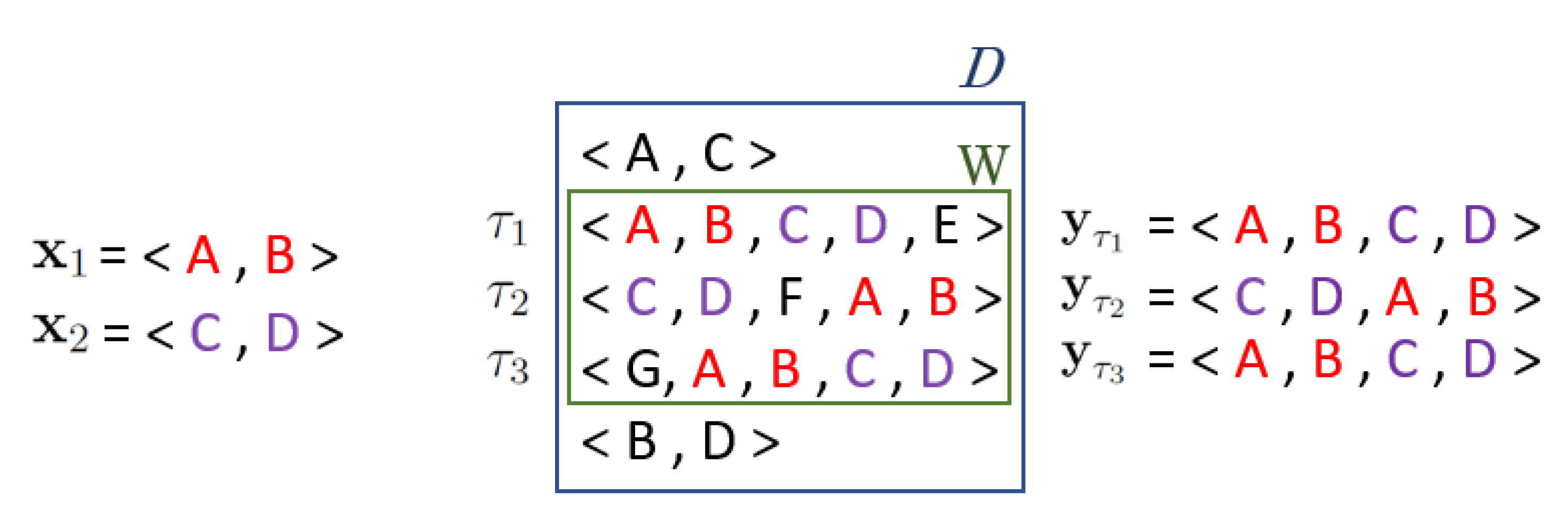
2.1. Sequential Pattern Mining
2.1.1. Frequent Sequential Pattern Mining
- contains a pair for every ;
- contains no pair such that ;
- for every , it holds .
- contains no pair such that ;
- contains all the pairs such that ;
- for every , it holds .
2.1.2. True Frequent Sequential Pattern Mining
- contains a pair for every ;
- contains no pair such that ;
- for every , it holds .
- contains no pair such that ;
- contains all the pairs such that ;
- for every , it holds .
2.2. VC-Dimension
2.3. Rademacher Complexity
2.4. Maximum Deviation
3. VC-Dimension of Sequential Patterns
- is the set of sequential transactions in the dataset;
- is a family of sets of sequential transactions such that for each sequential pattern p, the set is the support set of p on .
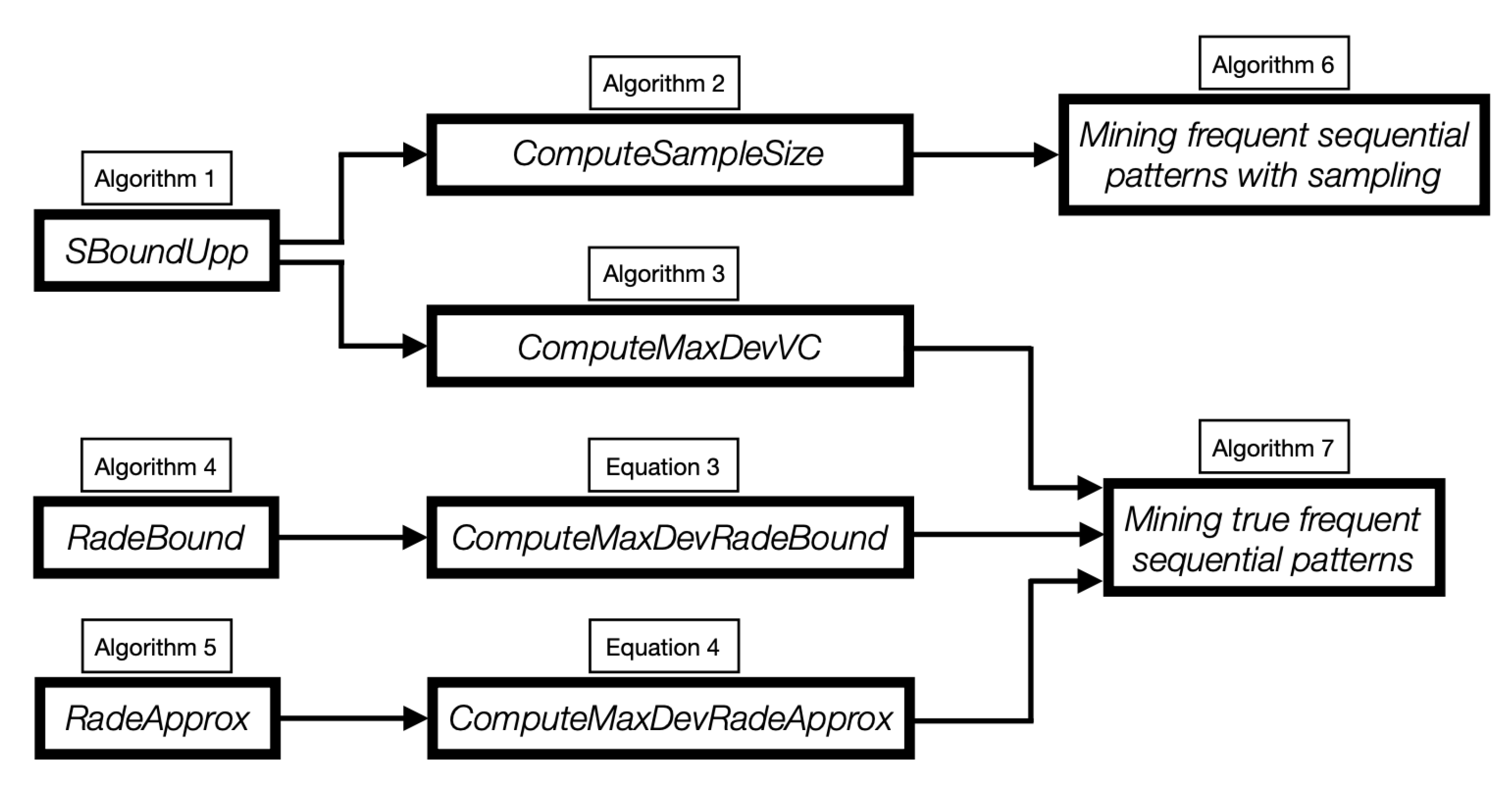
| Algorithm1: SBoundUpp(): computation of an upper bound on the s-bound. |
 |
3.1. Compute the Sample Size for Frequent Sequential Pattern Mining
| Algorithm2: ComputeSampleSize(): computation of the sample size such that with probability . |
| Data: Dataset ; . Result: The sample size m. 1 SBoundUpp(); 2 ; 3 return m; |
3.2. Compute an Upper Bound to the Max Deviation for the True Frequent Sequential Patterns
| Algorithm3: ComputeMaxDevVC(): computation of an upper bound on the max deviation for the true frequent sequential pattern mining problem. |
| Data: Dataset ; . Result: Upper bound to the max deviation . 1 SBoundUpp(); 2 ; 3 return ; |
4. Rademacher Complexity of Sequential Patterns
4.1. An Efficiently Computable Upper Bound to the Rademacher Complexity of Sequential Patterns
| Algorithm4: RadeBound(): algorithm for bounding the empirical Rademacher complexity of sequential patterns |
 |
4.2. Approximating the Rademacher Complexity of Sequential Patterns
| Algorithm5: RadeApprox(): algorithm for approximating the Rademacher complexity of sequential patterns. |
 |
5. Sampling-Based Algorithm for Frequent Sequential Pattern Mining
| Algorithm6: Sampling-Based Algorithm for Frequent Sequential Pattern Mining. |
| Data: Dataset ; ; . Result: Set that is an -approximation (resp. a FPF -approximation) to with probability . 1 ComputeSampleSize( 2 sample of m transactions taken independently at random with replacement from ; 3 ; /* resp. to obtain a FPF -approximation */ 4 return; |
6. Algorithms for True Frequent Sequential Pattern Mining
| Algorithm7: Mining the True Frequent Sequential Patterns. |
| Data: Dataset ; ; Result: Set that is a FPF -approximation (resp. -approximation) to with probability . 1 ComputeMaxDeviationBound(); 2 ; /* resp. to obtain a -approximation */ 3 return; |
7. Experimental Evaluation
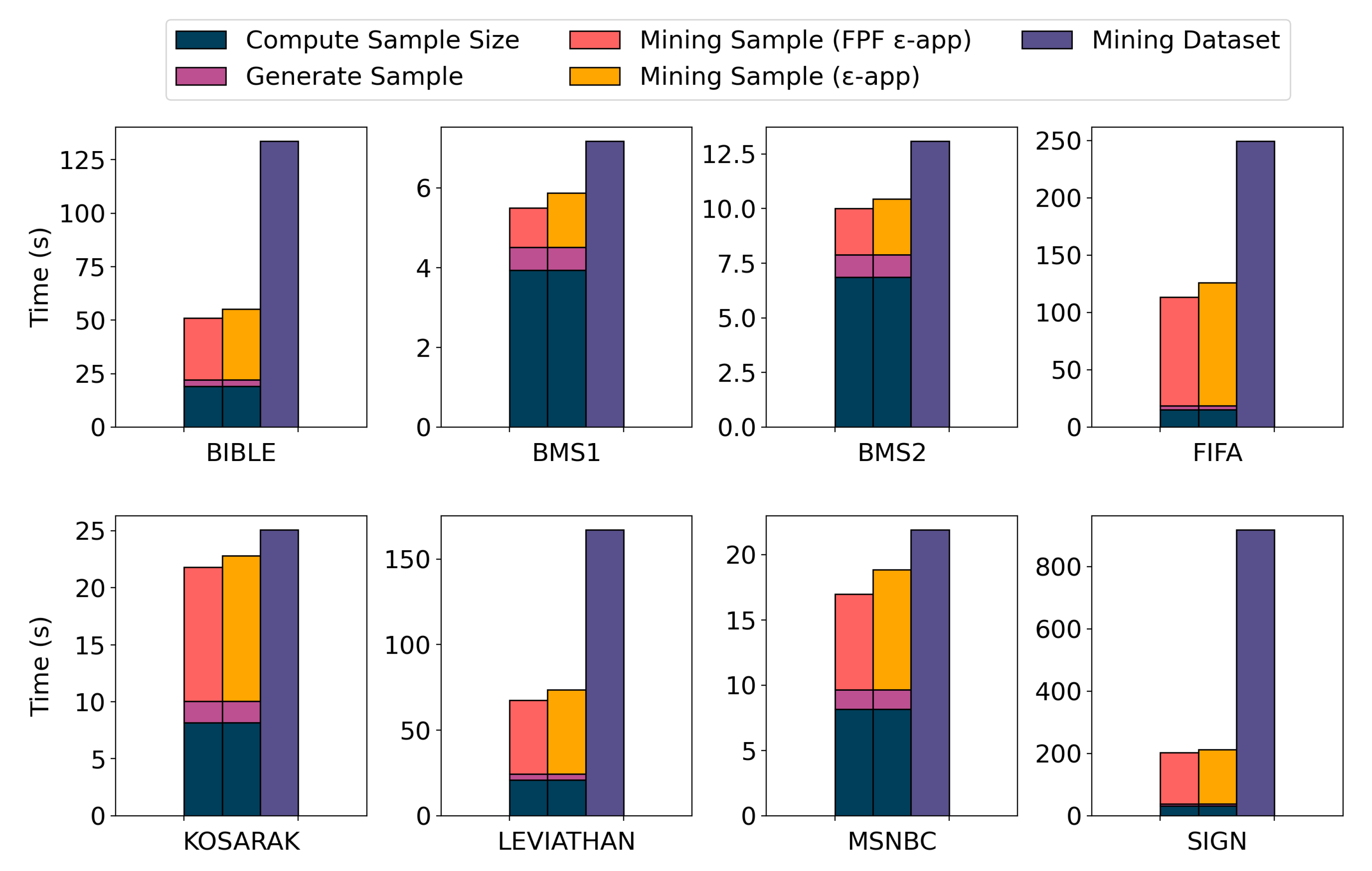
- Assess the performance of our sampling algorithm. In particular, to asses whether with probability the sets of frequent sequential patterns extracted from samples are -approximations, for the first strategy, and FPF -approximations, for the second one, of . In addition, we compared the performance of the sampling algorithm with the ones to mine the full datasets in term of execution time.
- Assess the performance of our algorithms for mining the true frequent sequential patterns. In particular, to assess whether with probability the set of frequent sequential patterns extracted from the dataset with the corrected threshold does not contain false positives, that is, it is a FPF -approximation of , for the first method, and contains all the TFSPs, that is, it is a -approximation of , for the second method. In addition, we compared the results obtained with the VC-dimension and with the Rademacher complexity, both used to compute an upper bound on the maximum deviation.
7.1. Implementation and Environment
7.2. Datasets
- BIBLE: a conversion of the Bible into sequence where each word is an item;
- BMS1: contains sequences of click-stream data from the e-commerce website Gazelle;
- BMS2: contains sequences of click-stream data from the e-commerce website Gazelle;
- FIFA: contains sequences of click-stream data from the website of FIFA World Cup 98;
- KOSARAK: contains sequences of click-stream data from an Hungarian news portal;
- LEVIATHAN: is a conversion of the novel Leviathan by Thomas Hobbes (1651) as a sequence dataset where each word is an item;
- MSNBC: contains sequences of click-stream data from MSNBC website and each item represents the category of a web page;
- SIGN: contains sign language utterance.
7.2.1. FSP Mining
7.2.2. TFSP Mining
7.3. Sampling Algorithm Results
7.4. True Frequent Sequential Patterns Results
8. Discussion
Author Contributions
Funding
Conflicts of Interest
Appendix A. Missing Proofs
References
- Agrawal, R.; Srikant, R. Mining sequential patterns. In Proceedings of the Eleventh International Conference on Data Engineering, Taipei, China, 6–10 March 1995; pp. 3–14. [Google Scholar]
- Vapnik, V.N.; Chervonenkis, A.Y. On the Uniform Convergence of Relative Frequencies of Events to Their Probabilities. In Measures of Complexity; Vovk, V., Papadopoulos, H., Gammerman, A., Eds.; Springer: Cham, Switzerland, 2015. [Google Scholar]
- Boucheron, S.; Bousquet, O.; Lugosi, G. Theory of classification: A survey of some recent advances. ESAIM Probab. Stat. 2005, 9, 323–375. [Google Scholar] [CrossRef]
- Riondato, M.; Upfal, E. Efficient discovery of association rules and frequent itemsets through sampling with tight performance guarantees. ACM Trans. Knowl. Discov. D 2014, 8, 20. [Google Scholar] [CrossRef]
- Riondato, M.; Upfal, E. Mining frequent itemsets through progressive sampling with rademacher averages. In Proceedings of the 21th ACM SIGKDD International Conference on Knowledge Discovery and Data Mining, New York, NY, USA, 22–27 August 2015; pp. 1005–1014. [Google Scholar]
- Raïssi, C.; Poncelet, P. Sampling for sequential pattern mining: From static databases to data streams. In Proceedings of the Seventh IEEE International Conference on Data Mining (ICDM 2007), Omaha, NE, USA, 28–31 October 2007; pp. 631–636. [Google Scholar]
- Riondato, M.; Vandin, F. Finding the true frequent itemsets. In Proceedings of the 2014 SIAM International Conference on Data Mining, Philadelphia, PA, USA, 28 April 2014; pp. 497–505. [Google Scholar]
- Servan-Schreiber, S.; Riondato, M.; Zgraggen, E. ProSecCo: Progressive sequence mining with convergence guarantees. Knowl. Inf. Syst. 2020, 62, 1313–1340. [Google Scholar] [CrossRef]
- Srikant, R.; Agrawal, R. Mining sequential patterns: Generalizations and performance improvements. In Advances in Database Technology–EDBT ’96, Proceedings of the International Conference on Extending Database Technology, Avignon, France, 25–29 March 1996; Springer: Berlin/Heidelberg, Germany, 1996; pp. 1–17. [Google Scholar]
- Pei, J.; Han, J.; Mortazavi-Asl, B.; Wang, J.; Pinto, H.; Chen, Q.; Dayal, U.; Hsu, M.C. Mining sequential patterns by pattern-growth: The prefixspan approach. IEEE Trans. Knowl. Data Eng. 2004, 16, 1424–1440. [Google Scholar]
- Wang, J.; Han, J.; Li, C. Frequent closed sequence mining without candidate maintenance. IEEE Trans. Knowl. Data Eng. 2007, 19, 1042–1056. [Google Scholar] [CrossRef]
- Pellegrina, L.; Pizzi, C.; Vandin, F. Fast Approximation of Frequent k-mers and Applications to Metagenomics. J. Comput. Biol. 2019, 27, 534–549. [Google Scholar] [CrossRef] [PubMed]
- Riondato, M.; Vandin, F. MiSoSouP: Mining interesting subgroups with sampling and pseudodimension. In Proceedings of the 24th ACM SIGKDD International Conference on Knowledge Discovery & Data Mining, London, UK, 19 July 2018; pp. 2130–2139. [Google Scholar]
- Al Hasan, M.; Chaoji, V.; Salem, S.; Besson, J.; Zaki, M.J. Origami: Mining representative orthogonal graph patterns. In Proceedings of the Seventh IEEE International Conference on Data Mining (ICDM 2007), Omaha, NE, USA, 28–31 October 2007; pp. 153–162. [Google Scholar]
- Corizzo, R.; Pio, G.; Ceci, M.; Malerba, D. DENCAST: distributed density-based clustering for multi-target regression. J. Big Data 2019, 6, 43. [Google Scholar] [CrossRef]
- Cheng, J.; Fu, A.W.c.; Liu, J. K-isomorphism: privacy preserving network publication against structural attacks. In Proceedings of the 2010 ACM SIGMOD International Conference on Management of Data, Indianapolis, Indiana, 6–11 June 2010; pp. 459–470. [Google Scholar]
- Riondato, M.; Upfal, E. ABRA: Approximating betweenness centrality in static and dynamic graphs with rademacher averages. ACM Trans. Knowl. Discov. D 2018, 12, 1–38. [Google Scholar] [CrossRef]
- Mendes, L.F.; Ding, B.; Han, J. Stream sequential pattern mining with precise error bounds. In Proceedings of the Eighth IEEE International Conference on Data Mining, Pisa, Italy, 15–19 December 2008; pp. 941–946. [Google Scholar]
- Pellegrina, L.; Riondato, M.; Vandin, F. SPuManTE: Significant Pattern Mining with Unconditional Testing. In Proceedings of the 25th ACM SIGKDD International Conference on Knowledge Discovery & Data Mining, Anchorage, AK, USA, 4–8 August 2019; pp. 1528–1538. [Google Scholar]
- Gwadera, R.; Crestani, F. Ranking Sequential Patterns with Respect to Significance. In Advances in Knowledge Discovery and Data Mining; Zaki, M.J., Yu, J.X., Ravindran, B., Pudi, V., Eds.; Springer: Berlin, Germany, 2010; Volume 6118. [Google Scholar]
- Low-Kam, C.; Raïssi, C.; Kaytoue, M.; Pei, J. Mining statistically significant sequential patterns. In Proceedings of the IEEE 13th International Conference on Data Mining, Dallas, TX, USA, 7–10 December 2013; pp. 488–497. [Google Scholar]
- Tonon, A.; Vandin, F. Permutation Strategies for Mining Significant Sequential Patterns. In Proceedings of the IEEE International Conference on Data Mining (ICDM), Beijing, China, 8–11 November 2019; pp. 1330–1335. [Google Scholar]
- Mitzenmacher, M.; Upfal, E. Probability and Computing: Randomization and Probabilistic Techniques in Algorithms and Data Analysis; Cambridge University Press: New York, NY, USA, 2017. [Google Scholar]
- Löffler, M.; Phillips, J.M. Shape fitting on point sets with probability distributions. In Algorithms–ESA 2009, Proceedings of the European Symposium on Algorithms, Copenhagen, Denmark, 7–9 September 2009; Springer: Berlin/Heidelberg, Germany, 2009; pp. 313–324. [Google Scholar]
- Li, Y.; Long, P.M.; Srinivasan, A. Improved bounds on the sample complexity of learning. J. Comput. Syst. Sci. 2001, 62, 516–527. [Google Scholar] [CrossRef]
- Shalev-Shwartz, S.; Ben-David, S. Understanding machine learning: From theory to algorithms; Cambridge University Press: New York, NY, USA, 2014. [Google Scholar]
- Egho, E.; Raïssi, C.; Calders, T.; Jay, N.; Napoli, A. On measuring similarity for sequences of itemsets. Data Min. Knowl. Discov. 2015, 29, 732–764. [Google Scholar] [CrossRef][Green Version]
- Fournier-Viger, P.; Lin, J.C.W.; Gomariz, A.; Gueniche, T.; Soltani, A.; Deng, Z.; Lam, H.T. The SPMF open-source data mining library version 2. In Machine Learning and Knowledge Discovery in Databases; Berendt, B., Ed.; Springer: Cham, Switzerland, 2016; Volume 9853, pp. 36–40. [Google Scholar]
- Johnson, S.G. The NLopt Nonlinear-Optimization Package. 2014. Available online: https://nlopt.readthedocs.io/en/latest/ (accessed on 10 April 2020).
- GitHub. VCRadSPM: Mining Sequential Patterns with VC-Dimension and Rademacher Complexity. Available online: https://github.com/VandinLab/VCRadSPM (accessed on 10 April 2020).
- SPMF Datasets. Available online: https://www.philippe-fournier-viger.com/spmf/index.php?link=datasets.php (accessed on 10 April 2020).


| Dataset | Size | Avg. Item-Length | Max. Item-Length | |
|---|---|---|---|---|
| BIBLE | 36,369 | 13,905 | 21.6 | 100 |
| BMS1 | 59,601 | 497 | 2.5 | 267 |
| BMS2 | 77,512 | 3340 | 4.6 | 161 |
| FIFA | 20,450 | 2990 | 36.2 | 100 |
| KOSARAK | 69,999 | 14,804 | 8.0 | 796 |
| LEVIATHAN | 5835 | 9025 | 33.8 | 100 |
| MSNBC | 989,818 | 17 | 4.8 | 14,795 |
| SIGN | 730 | 267 | 52.0 | 94 |
| Dataset | Max_Abs_Err (× | Avg_Abs_Err (× | -approx (%) | FPF -approx (%) | ||
|---|---|---|---|---|---|---|
| BIBLE | 0.1 | 0.24 | 9.33 | 7.47 | 100 | 100 |
| BMS1 | 0.012 | 0.17 | 5.45 | 4.70 | 100 | 100 |
| BMS2 | 0.012 | 0.16 | 4.08 | 3.14 | 100 | 100 |
| FIFA | 0.25 | 0.50 | 8.68 | 7.07 | 100 | 100 |
| KOSARAK | 0.02 | 0.52 | 7.18 | 4.95 | 100 | 100 |
| LEVIATHAN | 0.15 | 0.30 | 9.19 | 7.84 | 100 | 100 |
| MSNBC | 0.02 | 0.37 | 4.33 | 3.63 | 100 | 100 |
| SIGN | 0.4 | 0.20 | 14.14 | 12.19 | 100 | 100 |
| Ground Truth | |TFSP| | Times FPs | Times FNs | |
|---|---|---|---|---|
| BIBLE | 0.1 | 174 | 50% | 100% |
| 0.05 | 774 | 100% | 100% | |
| BMS1 | 0.025 | 13 | 50% | 0% |
| 0.0225 | 17 | 0% | 25% | |
| BMS2 | 0.025 | 10 | 0% | 0% |
| 0.0225 | 11 | 0% | 0% | |
| KOSARAK | 0.06 | 23 | 100% | 0% |
| 0.04 | 41 | 50% | 25% | |
| LEVIATHAN | 0.15 | 225 | 75% | 100% |
| 0.1 | 651 | 100% | 100% | |
| MSNBC | 0.02 | 97 | 75% | 25% |
| 0.015 | 143 | 100% | 50% |
| Dataset | |||||||||
|---|---|---|---|---|---|---|---|---|---|
| avg | max | std (×) | avg | max | std (×) | avg | max | std (×) | |
| BIBLE | 0.0339 | 0.0340 | 0.1 | 0.0747 | 0.0748 | 0.1 | 0.0207 | 0.0223 | 1.5 |
| BMS1 | 0.0194 | 0.0197 | 0.3 | 0.0287 | 0.0294 | 0.6 | 0.0136 | 0.0153 | 1.0 |
| BMS2 | 0.0194 | 0.0196 | 0.1 | 0.0202 | 0.0207 | 0.5 | 0.0107 | 0.0115 | 0.5 |
| KOSARAK | 0.0334 | 0.0335 | 0.1 | 0.0957 | 0.0972 | 1.5 | 0.0145 | 0.0164 | 1.5 |
| LEVIATHAN | 0.0847 | 0.0850 | 0.3 | 0.1878 | 0.1904 | 1.6 | 0.0569 | 0.0636 | 5.5 |
| MSNBC | 0.0089 | 0.0090 | 0.1 | 0.0252 | 0.0257 | 0.9 | 0.0035 | 0.0041 | 0.4 |
| Ground Truth | |TFSP| | Times FPs in FSP() | |FSP(/ |TFSP| | Times FPs in FSP() | |FSP(/ |TFSP| | |
|---|---|---|---|---|---|---|
| BIBLE | 0.1 | 174 | 0 % | 0.55 | 0 % | 0.68 |
| 0.05 | 774 | 0 % | 0.32 | 0 % | 0.47 | |
| BMS1 | 0.025 | 13 | 0 % | 0.38 | 0 % | 0.48 |
| 0.0025 | 17 | 0 % | 0.29 | 0 % | 0.43 | |
| BMS2 | 0.025 | 10 | 0 % | 0.13 | 0 % | 0.20 |
| 0.0025 | 11 | 0 % | 0.18 | 0 % | 0.18 | |
| KOSARAK | 0.06 | 23 | 0 % | 0.41 | 0 % | 0.73 |
| 0.04 | 41 | 0 % | 0.43 | 0 % | 0.74 | |
| LEVIATHAN | 0.15 | 225 | 0 % | 0.30 | 0 % | 0.41 |
| 0.1 | 651 | 0 % | 0.18 | 0 % | 0.30 | |
| MSNBC | 0.02 | 97 | 0 % | 0.56 | 0 % | 0.77 |
| 0.015 | 143 | 0 % | 0.50 | 0 % | 0.76 |
| Ground Truth | |TFSP| | Times FNs in FSP() | |TFSP|/ |FSP( | Times FNs in FSP() | |TFSP|/ |FSP( | |
|---|---|---|---|---|---|---|
| BIBLE | 0.1 | 174 | 0 % | 0.42 | 0 % | 0.63 |
| 0.05 | 774 | 0 % | 0.09 | 0 % | 0.33 | |
| BMS1 | 0.025 | 13 | 0 % | 0.07 | 0 % | 0.21 |
| 0.0025 | 17 | 0 % | 0.04 | 0 % | 0.19 | |
| BMS2 | 0.025 | 10 | 0 % | 0.03 | 0 % | 0.32 |
| 0.0025 | 11 | 0 % | 0.01 | 0 % | 0.19 | |
| KOSARAK | 0.06 | 23 | 0 % | 0.30 | 0 % | 0.64 |
| 0.04 | 41 | 0 % | 0.04 | 0 % | 0.49 | |
| LEVIATHAN | 0.15 | 225 | 0 % | 0.12 | 0 % | 0.30 |
| 0.1 | 651 | 0 % | 0.01 | 0 % | 0.13 | |
| MSNBC | 0.02 | 97 | 0 % | 0.42 | 0 % | 0.77 |
| 0.015 | 143 | 0 % | 0.24 | 0 % | 0.65 |
© 2020 by the authors. Licensee MDPI, Basel, Switzerland. This article is an open access article distributed under the terms and conditions of the Creative Commons Attribution (CC BY) license (http://creativecommons.org/licenses/by/4.0/).
Share and Cite
Santoro, D.; Tonon, A.; Vandin, F. Mining Sequential Patterns with VC-Dimension and Rademacher Complexity. Algorithms 2020, 13, 123. https://doi.org/10.3390/a13050123
Santoro D, Tonon A, Vandin F. Mining Sequential Patterns with VC-Dimension and Rademacher Complexity. Algorithms. 2020; 13(5):123. https://doi.org/10.3390/a13050123
Chicago/Turabian StyleSantoro, Diego, Andrea Tonon, and Fabio Vandin. 2020. "Mining Sequential Patterns with VC-Dimension and Rademacher Complexity" Algorithms 13, no. 5: 123. https://doi.org/10.3390/a13050123
APA StyleSantoro, D., Tonon, A., & Vandin, F. (2020). Mining Sequential Patterns with VC-Dimension and Rademacher Complexity. Algorithms, 13(5), 123. https://doi.org/10.3390/a13050123